 Li Quanjun
 Sun Huazhong1
- 1State Grid Weifang Electric Power Company, Weifang, Shandong, China
- 2School of Electrical Automation and Information Engineering of Tianjin University, Tianjin, China
The uncertainties of distribution generations (DGs) and loads lead to severe voltage fluctuations in active distribution networks (ADNs). Meanwhile, energy storage systems (ESSs) and static var compensators (SVCs) can mitigate the uncertainties of power injections by regulating the active and reactive power. Considering the variations of multiple uncertain factors, this paper proposes a complex affine arithmetic (CAA) based uncertain sensitivity analysis method of voltage fluctuations in ADNs. First, affine models of active and reactive power injections are established. The correlations of noisy symbols are used to reflect the mitigation effects of ESSs and SVCs on the uncertainties introduced by DGs and loads. Next, sensitivity indicators of voltage fluctuations are defined based on the transitivity of noisy symbols. Then, a calculation method for sensitivity indicators based on the micro-increments of coefficients is proposed. Combined with the obtained indicators, a fast sensitivity method for calculating interval values of voltages is further proposed. The modified IEEE 33-bus system is tested to validate the accuracy and efficiency of the proposed method by comparison with the continuous utilization of power flow method. Moreover, the 292-bus system is tested to validate its applicability in a large distribution system. Facts have proved that this method improves the efficiency and reliability of calculations, and in different scenarios, it can achieve fast calculation of nodes and online analysis of the voltage fluctuation range in uncertain environments, provides an effective tool for voltage quality management in active distribution networks.
1 Introduction
The stochastic and intermittent characteristics of renewable energy resources cause the uncertainties of distributed generations (DGs) in active distribution networks (ADNs) (Alonso-Travesset et al., 2022). Meanwhile, the fluctuations of load demands have increased the uncertainties to some extent (Zhang et al., 2023). The uncertainties will induce severe voltage fluctuations in ADNs. The integration of energy storage systems (ESSs) and static var compensators (SVCs) can mitigate the uncertainties of power injections by regulating the active and reactive power, which will reduce the levels of voltage fluctuations. Considering the variations of multiple uncertain factors, an uncertain sensitivity analysis method can help to control critical nodes and uncertain factors in such an uncertain environment.
The sensitivity analysis method generally uses the differential relationship of variables to indicate the sensitivity of output variables to the variations of input variables (Shang et al., 2021). According to different physical interpretations of variables, multiple sensitivity indicators are defined (Chang et al., 2022). For instance, the indicators
Traditionally, there are three typical methods for calculating sensitivity indicators of voltages.
The first type is the Jacobian matrix method. In the process of Calculating the power flow of the Newtonian method, the Jacobian matrix J contains the partial derivatives of the node’s net injection of active and reactive power with respect to the voltage. Through the inversion operation of the matrix, the sensitivity of the voltage to the change of the node’s net injection of active and reactive power can be obtained. Indicators (Alzaareer et al., 2020; Song et al., 2020; Munikoti et al., 2021). When the Newtonian power flow calculation reaches the convergence state, the obtained Jacobian matrix and inversion operation can be used to obtain the voltage sensitivity index. Literature (Mlilo et al., 2021) considers the random output characteristics of wind power, uses the Jacobian matrix method to calculate the voltage sensitivity index, and combines the K-means clustering method and joint sensitivity to establish a voltage sensitivity analysis scenario.
The second type is the incremental method. The incremental method can also be called the perturb-and-observe approach. By giving a small change in the input variable, the change in the output variable is observed to calculate the voltage sensitivity index (Shuai et al., 2021; Gupta and Paolone, 2023). The incremental method is simple and easy to implement, and obtains high-precision voltage sensitivity indicators by making the changes in the net injected active and reactive power of the node tend to zero. From a simulation perspective, the incremental method is easy to implement. Literature (Alvarado-Barrios et al., 2020) developed a voltage sensitivity analysis software for the distribution network based on the incremental method, and set the increment of the node’s net injected power to 0.5% of the average load level. To 2%, a high-precision voltage sensitivity index that meets the requirements is obtained. The incremental method has high adaptability to various functions or power flow algorithms, but when the input variables change, it is necessary to calculate and observe the changes in the output variables, which increases the overall calculation amount.
The third category is topological analysis method. The topological analysis method is based on the network topology, applies Tellegen’s theorem, and combines the adjoint network theory to calculate the voltage sensitivity index (Bandler and El-Kady, 1980; Bai et al., 2020). Literature (Wang et al., 2018) elaborates on the adjoint network theory and the sensitivity calculation method based on the generalized Tellegen theorem, and applies the voltage sensitivity index to the vulnerability assessment of the power grid. Literature (Ye et al., 2021) proposed a new calculation method for voltage sensitivity index based on changes in the net injected active and reactive power of nodes in a three-phase unbalanced distribution network. This method calculates ABCD parameters based on network topology and realizes fast online calculation of voltage sensitivity indicators. The topological analysis method usually requires a power flow solution of a reference state in order to establish a specific adjoint network, and then use the network topology parameters to obtain the voltage sensitivity index.
The method based on the Jacobian matrix provides accurate results and is suitable for stability analysis, but requires recalculation when system conditions change, which is computationally intensive. The perturbation and observation method is easy to operate and suitable for rapid sensitivity assessment, but may not be as accurate as the Jacobian method. The method based on circuit theory has a solid theoretical foundation and is suitable for education and in-depth research, but the preparation work is more complicated.
However, considering voltage fluctuations caused by the uncertainties in ADNs, voltages become uncertain values with the lower and upper bounds, instead of deterministic point values. Each change in node voltage covers all point values in the range of change. But in previous sensitivity analysis, the variation only reflects the deviation between point values. Thus, new methods need to be studied to handle uncertain variables in the sensitivity analysis of voltage fluctuations.
Faced with the uncertainty problem, affine arithmetic (AA) can effectively deal with uncertain variables with the lower and upper bounds (Ruiz-Rodriguez et al., 2020). Compared with interval arithmetic, AA performs better in terms of more compact solution region and lower conservativeness. Further, AA is extended into the complex plane and complex affine arithmetic (CAA) is developed (Manson, 2005; Wang et al., 2019). Since AA and CAA have been used to handle the uncertainty problem in power systems, existing researches mainly focus on the uncertain power flow calculation (Guerrero et al., 2020; Meinecke et al., 2020; Tang et al., 2020; Zeynali et al., 2020; Wang et al., 2021). In addition, reference (Zhang et al., 2022) proposed a reactive power optimization method while using AA to handle interval uncertainties. CAA can keep track of correlations among uncertain variables, which helps to carry out sensitivity analysis in uncertain environments.
Therefore, a CAA based uncertain sensitivity analysis method of voltage fluctuations in ADNs is proposed. The main contributions are highlighted as follows.
1) CAA is used to quantify the uncertainties introduced by DGs and loads, as well as the mitigation effects of ESSs and SVCs. Affine models of active and reactive power injections are established based on the correlations of noisy symbols. Further, considering the variations of multiple factors, sensitivity indicators of voltage fluctuations are defined based on the transitivity of noisy symbols.
2) A calculation method for sensitivity indicators based on the micro-increments of coefficients is proposed. In the calculation process, an improved forward-backward sweep power flow based on CAA is used to calculate the voltages in affine form. The obtained indicators can quantitatively reflect the sensitivity of voltage fluctuations to the variations of uncertain factors.
3) A fast sensitivity method for calculating interval values of voltages is proposed. The proposed method avoids the continuous utilization of power flow algorithm while guaranteeing the accuracy and efficiency of calculation.
The rest of the paper is organized as follows. Section 2 describes the complex affine arithmetic. Section 3 establishes the affine models of active and reactive power injections considering correlations. Section 4 proposes a CAA based uncertain sensitivity analysis method of voltage fluctuations in ADNs. Section 5 conducts the case study and discusses the results. Finally, Section 6 draws the main conclusions.
2 Complex affine arithmetic
2.1 Mathematical theory
The complex affine variable is represented by a linear combination of the center value and a series of noise terms [19]. A complex affine variable is defined as in (1).
Each noisy symbol represents an uncertain factor and the corresponding coefficient reflects the magnitude of fluctuation around the center value.
Given two complex affine variables
In the above formula (2) and formula (3),
The main challenge is to find the optimal approximation for non-affine terms as in (Shang et al., 2021)-(4). The derivation and proof of basic operations can be referred to [20]. In the calculation process, the number of error terms will increase with the existence of non-affine terms.
2.2 Correlation and transitivity properties of noisy symbols
In this paper, uncertain sensitivity analysis of voltage fluctuations mainly relies on the correlation and transitivity properties of noisy symbols. In CAA, correlations among complex affine variables can be reflected by coexisting noisy symbols. Meanwhile, the coefficients of noisy symbols can reflect the uncertainty level of each complex affine variable.
For a multivariate function f with n input variables in affine form, the transitivity of noisy symbols is shown as in (5–7).
In the formula,
Assuming that there are m non-affine operations in the function, noise terms of
For each uncertain variable
When the uncertainty levels of input variables changes, the new complex affine variables are denoted as:
In the formula (8),
Then, the output variable is updated by (9).
The main effects of the variations on the output variable can be quantified by the corresponding coefficients of noisy symbols (
3 Affine models of active and reactive power injections considering correlations
Considering the uncertainties of DGs and loads, as well as the mitigation effects of ESSs and SVCs, affine models of active and reactive power injections are built. The correlations of noisy symbols are used to reflect the mitigation effects of ESSs and SVCs on uncertainties introduced by DGs and loads.
3.1 Affine model of active power injection
The affine model of active power injection of phase φ at node i is shown as in (10).
The model considers the active power of loads, DGs, and ESSs. The load power is regarded as the positive direction, and the positive value of
Then, the affine model of each part in (10) is built, separately. Firstly, considering the uncertainties of loads, the interval model of load active power is shown as in (12), in which
Secondly, considering the uncertainties of DGs, affine models of wind turbine generator and photovoltaic system are built based on meteorological conditions and power equations (23). The interval model of DG active power is shown as in (14), in which
Thirdly, for the ESS connected at node i, the interval model of active power is shown as in (16), in which
On the one hand, noisy symbols of DGs and loads are marked with “+“, which reflects the uncertainty sources. On the other hand, noisy symbols of ESSs are marked with “-“, which reflects the mitigation effects on uncertainties. Since the coefficients of
3.2 Affine model of reactive power injection
Considering the reactive power of loads, DGs, and SVCs, the affine model of reactive power injection of phase φ at node i is shown as in (19). The value of
The affine model of each part in (19) is built, separately. Firstly, Eq. 20 shows the interval model of load reactive power with the lower and upper bounds. Then, the affine model is obtained by (21).
Secondly, assuming that DGs are operating at a constant power factor, the affine model of DG reactive power is obtained by (22).
Thirdly, the interval model of SVC reactive power is shown as in (23), in which
Noisy symbols of SVCs are marked with “-“, which reflects the mitigation effects on uncertainties. SVCs can provide reactive power for loads and mitigate the uncertainties introduced by loads. Since the coefficients of
4 Uncertain sensitivity analysis of voltage fluctuations based on CAA
4.1 Sensitivity indicators of voltage fluctuations to active and reactive power injections
Based on the transitivity of noisy symbols, sensitivity equations of voltage fluctuations with complex affine variables are established. The equations take into account not only the variations of uncertainty levels of DGs and loads, but also the variations of mitigation levels of ESSs and SVCs.
Assuming that there are q noise symbols introduced by the uncertainties of power injections, the calculation process from power injections to voltages is shown as in (26). The number of buses is n. Considering the variations of multiple factors, affine valued voltages at the initial and current states are obtained.
In the formula,
Specifically, the variations of active and reactive power injections are obtained by (27).
In the formula,
The main noise terms of
Further, the formula is represented by the real and imaginary parts. For instance, the expression of
The level of voltage fluctuation at node i is denoted as
Then, indicators are defined for evaluating the sensitivity of voltage fluctuations to the above variations in power injections.
4.1.1 Sensitivity indicator towards individual variation
The voltage fluctuation at node i is affected by the variations of multiple factors in power injections as shown in (27). Considering the variations of uncertainty levels of DGs and loads, as well as mitigation levels of ESSs and SVCs, the variations of corresponding coefficients can be expressed as
The effect of individual variation on the voltage fluctuation at node i can be evaluated by the transitivity of corresponding noisy symbol. Assuming that
Then, sensitivity indicator of the voltage fluctuation at node i to individual variation is defined as in (32).
In the formula,
4.1.2 Sensitivity indicator towards total variations
Considering total variations of multiple factors, the variation of the level of voltage fluctuation at node i is calculated by (33).
Then, sensitivity indicator of the voltage fluctuation at node i to total variations is defined as in (34).
In the formula,
4.2 Calculation method for sensitivity indicators based on the micro-increments of coefficients
4.2.1 Micro-increments of coefficients of noisy symbols
Eqs 32, 34 use the general form
In [12], the sensitivity analysis of voltages with point values is studied and a sensible strategy is to set each micro-increment as a percentage of load power. It is demonstrated that when each micro-increment is set as 0.5%–2% of load power, the obtained results have high accuracy. In this paper, the micro-increment is set as 1% of the uncertainty level or mitigation level of each factor. That is, each micro-increment is 1% of the coefficient of corresponding noisy symbol in the affine model of each factor.
4.2.2 CAA-based improved forward-backward sweep power flow
In the calculation process of sensitivity indicators, an improved forward-backward sweep power flow based on CAA is used to calculate voltages in affine form. Sensitivity indicators are further calculated based on the obtained coefficients of noisy symbols.
In previous CAA based forward-backward sweep power flow [23], a brand new noisy symbol is generated after approximation for each non-affine operation. Meanwhile, voltages and currents are updated repeatedly in the iterative process. As a result, numerous error noise terms are continually generated. The redundancy of error noise terms affects the clarity of sensitivity-related coefficients.
Therefore, a cutting method for error noise terms of voltages and currents is proposed. The coefficients of error noisy symbols are merged by summing the absolute values of their real and imaginary parts, respectively. Since the coefficients of error noisy symbols are extremely smaller than those of main noisy symbols, it guarantees the completeness of true solutions and has little effect on the conservativeness.
In the process of forward and backward sweep, the improvement mainly lies in de-redundancy of error noise terms of voltages and currents. Figure 1 shows the topology of an ADN with DGs, loads, ESSs, and SVCs.
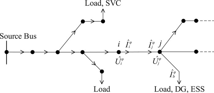
FIGURE 1. Topology of an ADN with DGs, loads, ESSs, and SVC.
For instance, in the process of forward sweep, the downstream voltage
4.2.3 Calculation process of sensitivity indicators
Combined with the improved forward-backward sweep power flow based on CAA, sensitivity indicators are calculated based on the micro-increments of coefficients of noisy symbols. The detailed process of calculation is as follows:
i) Initialize the network parameters such as node number and line impedance. Based on the affine models of DGs, loads, ESSs, and SVCs, active and reactive power injections at the initial state are obtained by (Song et al., 2020) and (19). Then, the initial voltages in affine form are calculated by the improved forward-backward sweep power flow based on CAA.
ii) For the variations of factors in active power injections, the micro-increments of coefficients of corresponding noisy symbols are set. Combined with the improved forward-backward sweep power flow based on CAA, sensitivity indicator of the voltage fluctuation at node i to individual variation in active power injections is calculated by (32).
iii) Similarly, for the variations of factors in reactive power injections, sensitivity indicator of the voltage fluctuation at node i to individual variation in reactive power injections is calculated by (32).
iv) Considering total variations of factors in power injections, the micro-increments of coefficients of corresponding noisy symbols are set. Then, combined with the improved forward-backward sweep power flow based on CAA, sensitivity indicator of the voltage fluctuation at node i to total variations is calculated by (34).
4.3 A fast sensitivity method for calculating voltage intervals
Based on the obtained sensitivity indicators, a fast sensitivity method for calculating interval values of voltages is further proposed. The proposed method takes into account actual variations of uncertainty levels of DGs and loads, as well as mitigation levels of ESSs and SVCs. According to sensitivity indicators and actual variations of factors, the variations of voltage fluctuations are obtained by a linear calculation model. The proposed method avoids the continuous utilization of the power flow algorithm to calculate interval values of voltages.
Considering actual variations of multiple factors in power injections, the variation of the absolute value of the kth coefficient of the voltage at node i is calculated by (38).
Then, the variation of the level of voltage fluctuation at node i is calculating by summing the variations of the absolute values of all coefficients, which is shown as in (39). Combined with the initial voltages in affine form, the voltages at current state are further obtained.
5 Case study
5.1 System parameters and initial state
Considering the uncertainties of DGs and loads, as well as the mitigation effects of ESSs and SVCs, the proposed method is verified by the modified IEEE 33-bus distribution system. Figure 2 shows the topology of the system with DGs, loads, ESSs, and SVCs.
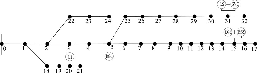
FIGURE 2. Topology of the modified IEEE 33-bus distribution system.
At the initial state, uncertainty levels of DGs and loads, as well as mitigation levels of ESSs and SVCs are set as follows:
1) DG1 and DG2 are integrated to buses 5 and 15, respectively. The interval of DG active power is [200,300] kW and the power factor is
2) L1 and L2 are the fluctuating loads at buses 20 and 30. The uncertainty level is
3) Bus 15 is connected with an ESS and the interval of ESS active power is [-60,-20] kW.
4) Bus 30 is connected with a SVC and the interval of SVC reactive power is [45,50] kvar.
Then, based on affine models of active and reactive power injections, the affine valued power of each DG, load, ESS, and SVC can be obtained as shown in Table 1.

TABLE 1. Power of DGs, loads, ESSs and SVCs in The Initial State.
5.2 Discussion of the results of uncertain sensitivity analysis
5.2.1 Sensitivity indicators of voltage fluctuations to DGs/loads
Firstly, considering the variation of uncertainty level of individual DG or load, sensitivity indicator of the voltage fluctuation at each bus is calculated. As for the real parts of voltages of phase A, Figure 3 shows sensitivity indicators of voltage fluctuations to active power of DG1 and L1. Secondly, considering total variations of DGs and loads, sensitivity indicator of the voltage fluctuation at each bus is calculated. Figure 4 shows sensitivity indicators of voltage fluctuations to all DGs and loads.
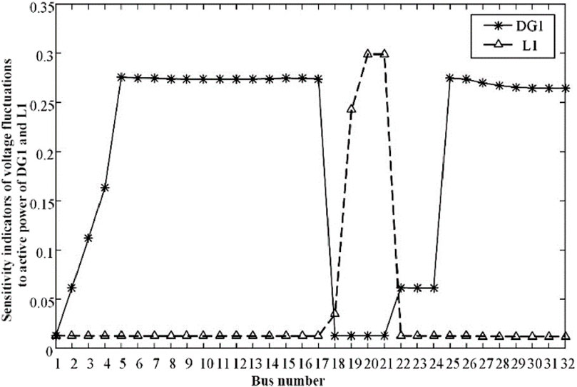
FIGURE 3. Sensitivity indicators of voltage fluctuations to active power of DG1/L1.
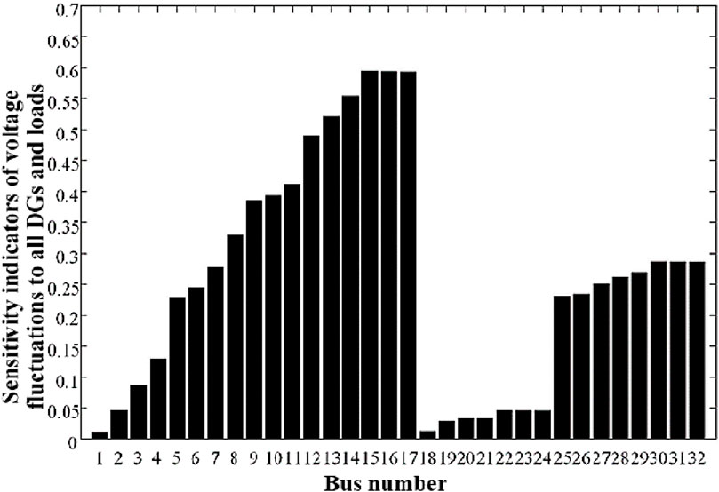
FIGURE 4. Sensitivity indicators of voltage fluctuations to all DGs and loads.
It can be seen from Figures 3, 4 that the obtained indicators can quantitatively reflect the sensitivity of voltage fluctuations to the variations of uncertainty levels of DGs and loads. The results show that buses close to the locations of DGs and loads have larger values of sensitivity indicators, which means that these buses are more sensitive to the variations of uncertain factors. Meanwhile, buses located at the end of the branch are more sensitive than those close to the source bus.
Taking into account the changes in uncertainty fluctuation levels of DG1, DG2, L1 and L2, the multi-factor uncertainty sensitivity index shown in Figure 4 represents the overall sensitivity of the voltage fluctuation range of each node to changes in all uncertainty fluctuation factors. For all uncertainty fluctuation factors in the distribution network shown in Figure 2, that is, DG1 and DG2 at nodes 5 and 15 and L1 and L2 at nodes 20 and 30, the results show that the uncertainty fluctuation factors are close to the location where the uncertainty fluctuation factors are connected and located on the branch. Nodes at the end of the road have larger multi-factor sensitivity index values and are more sensitive to changes in uncertainty fluctuation factors in the network; nodes far away from the access location of uncertainty fluctuation factors and close to the source node have smaller multi-factor sensitivity index values. The overall sensitivity to changes in uncertainty fluctuation factors in the network is low.
5.2.2 Sensitivity indicators of voltage fluctuations to ESSs/SVCs
The integration of ESSs and SVCs can mitigate the uncertainties of power injections. Considering the variation of the mitigation level of individual ESS or SVC, sensitivity indicator of the voltage fluctuation at each bus is calculated. Figure 5 shows sensitivity indicators of voltage fluctuations to individual ESS and SVC. Then, considering total variations of ESSs and SVCs, sensitivity indicator of the voltage fluctuation at each bus is calculated. Figure 6 shows sensitivity indicators of voltage fluctuations to all ESSs and SVCs.
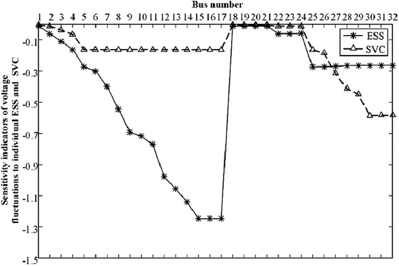
FIGURE 5. Sensitivity indicators of voltage fluctuations to individual ESS/SVC.
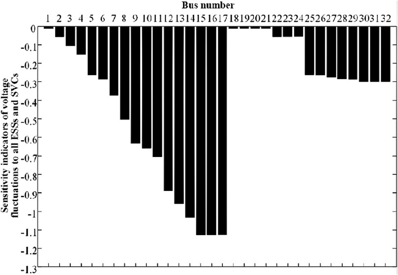
FIGURE 6. Sensitivity indicators of voltage fluctuations to all ESSs and SVCs.
As for the variations of mitigation levels of ESSs and SVCs, the values of sensitivity indicators are negative. As the mitigation levels increase, the levels of voltage fluctuations decrease. The results show that buses close to the locations of ESSs and SVCs have larger absolute values of sensitivity indicators. Similarly, buses located at the end of the branch are more sensitive than those close to the source bus.
The multi-factor uncertainty sensitivity index shown in Figure 6 represents the overall sensitivity of the voltage fluctuation range of each node to changes in all uncertainty reduction factors. For all uncertainty reduction factors in the distribution network shown in Figure 2, the results further show that nodes close to the access location of the uncertainty reduction factors and located at the end of the branch have a larger absolute value of the sensitivity index, which has a greater impact on the uncertainty in the network. Changes in reduction factors are more sensitive; nodes that are far away from the access location of uncertainty reduction factors and close to the source node have a smaller absolute value of the sensitivity index and are less affected by changes in uncertainty reduction factors in the network.
5.2.3 Comparative analysis
Based on the initial state, 6 scenarios are set considering actual variations of uncertainty levels of DGs and loads, as well as mitigation levels of ESSs and SVCs. The interval values of voltages are calculated and the results are compared between the proposed sensitivity method (Method 1) and the continuous utilization of the power flow method (Method 2).
In scenarios 1-3, uncertainty levels of DG1, DG2, L1, and L2 gradually increase based on the initial state. Specifically, the fluctuation levels around central values increased by 2%, 4%, and 6%, respectively. In scenarios 4-6, uncertainty levels of DGs and loads are the same as in scenario 3. The intervals of ESS active power are [-65,-15] kW [-70,-10] kW, and [-75,-5] kW, respectively. The intervals of SVC reactive power are [43,52] kvar [41,54] kvar, and [39,56] kvar, respectively.
Considering the variations of multiple factors, the variation of the level of voltage fluctuation at node i can be quantified by (33). As for the real parts of voltages of phase A, Figure 7 shows the variations of the levels of voltage fluctuations at buses 17 and 27. Figure 8 shows the interval values of voltages calculated by the two methods.
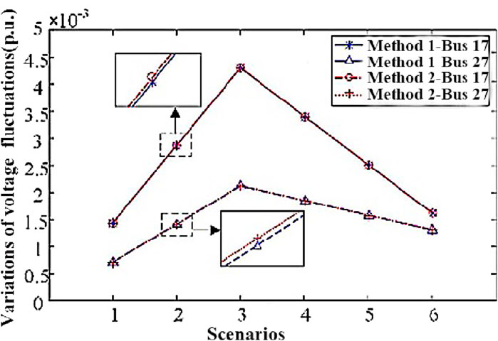
FIGURE 7. Variations of the levels of voltage fluctuations in different scenarios.
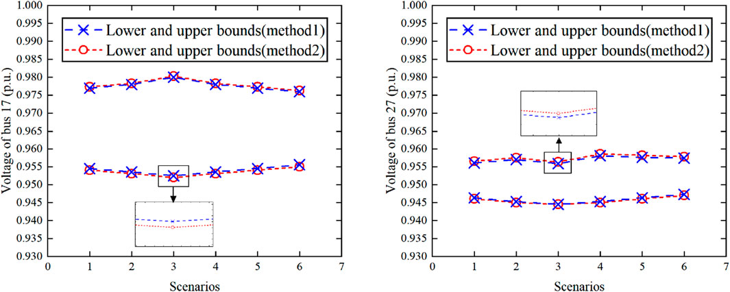
FIGURE 8. Interval values of voltages in different scenarios.
Then, based on the complex affine voltage of each node in the starting state and the change in voltage fluctuation level in each scene, the proposed method is used to obtain the voltage fluctuation interval after the scene change. Taking nodes 17 and 27 as an example, Figure 8 shows the fluctuation range of the real part of phase A voltage obtained by the two methods in each scenario, including its lower and upper bounds. Figure 9 shows the deviation values of voltage fluctuation level changes in various scenarios.
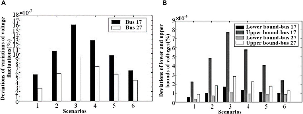
FIGURE 9. Deviations of the proposed method. (A) shows the deviation value of the voltage fluctuation level change of nodes 17 and 27 in various scenarios. (B) shows the deviation values of the upper and lower bounds of the voltage fluctuation range of nodes 17 and 27 in various scenarios.
As can be seen from Figures 7, 8, the change in voltage fluctuation level under each scenario and the voltage fluctuation interval after the scenario change are obtained through the proposed method. The results show that with the gradual increase in the uncertainty level of DG and load in scenarios 1-3, the voltage fluctuation level of each node gradually increases, and the voltage fluctuation range gradually expands; as the ESS and SVC active power in scenarios 4-6 And the gradual increase of the reactive power adjustment range has a certain effect on reducing the voltage fluctuation level, and the voltage fluctuation range gradually decreases.
The results show that with the increase of uncertainty levels of DGs and loads in scenarios 1-3, the levels of voltage fluctuations gradually increase. Meanwhile, with the increase of mitigation levels of ESSs and SVCs in scenarios 4-6, the levels of voltage fluctuations gradually decrease. By comparison, the results obtained by the two methods are very close. The difference can be found after sufficient amplification, which validates the accuracy of the proposed method.
Further, compared with method 2, Figure 9A shows deviations of the variations of the levels of voltage fluctuations obtained by method 1. Figure 9B shows deviations of the lower and upper bounds of voltages obtained by method 1.
It can be seen that as for deviations of voltage fluctuations at buses 17 and 27, the maximum value is within 0.02%. As for deviations of the upper and lower bounds of voltages, the maximum value is within 0.01%. The results further validate the accuracy of the proposed method. Meanwhile, the proposed method avoids the continuous utilization of the power flow algorithm, which guarantees the efficiency of calculation.
5.2.4 Applicability in a large distribution network
To validate the applicability in a large distribution network, the proposed method is tested on the 292-bus distribution system. The topology and technical data can be referred to (Wang and Wang, 2014).
At the initial state, uncertainty levels of DGs and loads, as well as mitigation levels of ESSs and SVCs are set as follows: 1) DG1-DG6 are integrated to buses 15, 50, 93, 110, 216, and 270. The interval of DG active power is [200,300] kW. 2) L1-L4 are the fluctuating loads at buses 13, 208, 230, and 268. The uncertainty level is
Considering the variations of multiple factors, sensitivity indicator of the voltage fluctuation at each bus to individual variation is calculated. Figure 10 shows sensitivity indicators of voltage fluctuations to active and reactive power of DG3 and L4. Figure 11 shows sensitivity indicators of voltage fluctuations to power of ESS2, ESS4, SVC1, and SVC2.
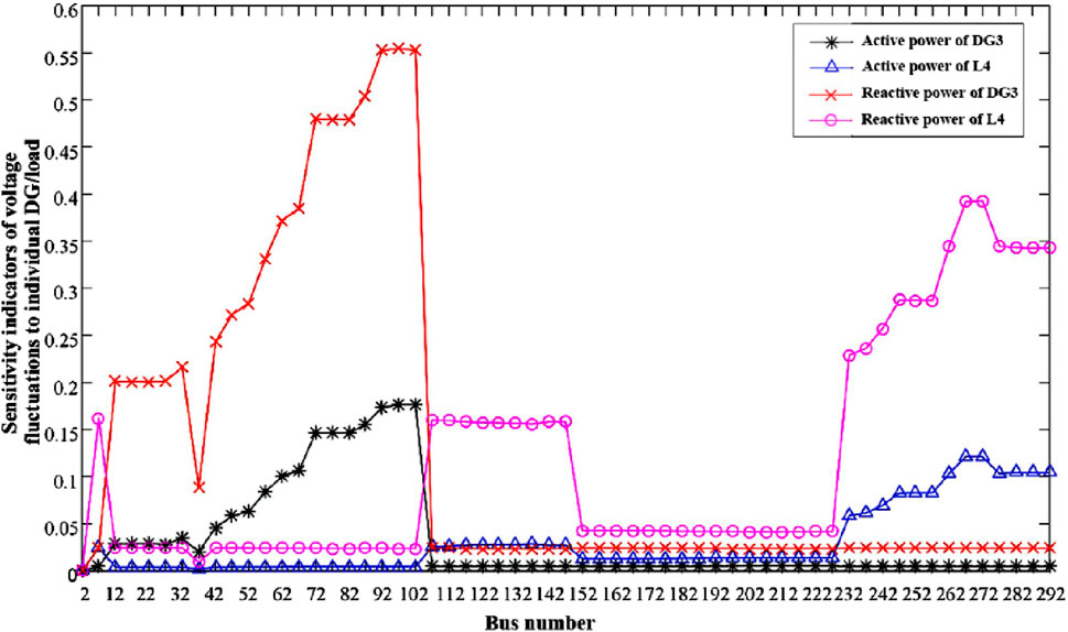
FIGURE 10. Sensitivity indicators of voltage fluctuations to individual DG/load.
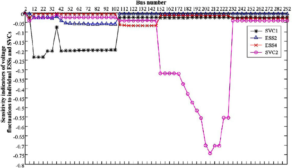
FIGURE 11. Sensitivity indicators of voltage fluctuations to individual ESS/SVC.
From the analysis in Figure 10, it can be seen that considering the changes in DG and load uncertainty fluctuation levels, the single-factor uncertainty sensitivity index curve of the node voltage fluctuation interval shows certain regular characteristics. First, nodes close to the access location of each uncertainty fluctuation factor have larger sensitivity index values, indicating that they are more sensitive to changes in the uncertainty fluctuation level of this factor; second, the transformers in the network are sensitive to uncertainty fluctuation factors. The impact of change has a certain blocking effect. For example, affected by changes in the uncertainty fluctuation level of load L4 at node 268, the sensitivity index values of nodes 228–292 are larger, and the closer to the node L4, the larger the sensitivity index value, indicating changes in the uncertainty fluctuation level of L4. The more sensitive the reaction. Secondly, the branch where nodes 103–147 are located is directly connected to the branch where L4 is located through node 7. Due to the distance, the sensitivity index value is lower than the index value of nodes 228–292. However, for the nodes on other branches, which are connected to the branch where L4 is located through the transformer at the head end of the branch, the sensitivity index is close to 0, indicating that it is basically not affected by changes in the uncertainty fluctuation level of L4.
From the analysis of Figure 11, it can be seen that in response to changes in the uncertainty reduction levels of ESS and SVC, the single-factor sensitivity indicators of each node’s voltage fluctuation range are all negative, indicating that as the uncertainty reduction level increases, the voltage fluctuation level increases. reduced. At the same time, the single-factor sensitivity index curve in the node voltage fluctuation range also shows certain regular characteristics. First, nodes close to the access location of each uncertainty reduction factor have a larger absolute value of the sensitivity index, indicating that they are more sensitive to changes in the uncertainty reduction level of this factor; second, the transformers in the network are sensitive to uncertainty reduction factors. The influence of changes also has a certain blocking effect. For nodes that are far away from the access point of the uncertainty reduction factor and separated by the transformer, the absolute value of the sensitivity index is close to 0, indicating that it is basically not affected by changes in the uncertainty reduction factor. For instance, considering the variation of the uncertainty level of L4 at bus 268, buses 228–292 are more sensitive. However, for buses on other branches, sensitivity indicators are close to 0 due to the blockage of transformers.
In order to better prove the effectiveness and reliability of the method proposed in this article, this paper compares the deviation values of the voltage fluctuation level change of the proposed method (Model 1) with the Jacobian matrix method (Model 2), perturb-and-observe, approach (Model 3) and topological analysis method I (Model 4) in six scenarios, and the statistical results are shown in Table 2.
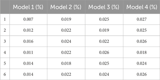
TABLE 2. Deviation value of voltage fluctuation level change of node 27 in various scenarios.
As can be seen from Table 2, the deviation values of the voltage fluctuation level changes of the method proposed in this article are within 0.02% in six scenarios. The deviation value of the results obtained by this method is extremely small, and the deviation value of the results in each scenario is lower than that of other scenarios. The model proposed in this article performs best among the four models, indicating that the model proposed in this article can quantitatively describe the sensitivity of the voltage fluctuation range to the uncertainty fluctuations of various factors, and helps to focus on controlling key nodes and key uncertainty factors.
6 Conclusion
This paper proposes a CAA-based sensitivity analysis method for ADN voltage fluctuation uncertainty. By analyzing the correlation and transitivity of noise symbols, it shows that ESS and SVC can reduce the voltage caused by distributed generation (DG) and load changes. Effectiveness in Fluctuations. This method introduces a new technology to calculate the voltage fluctuation sensitivity index through the micro-increment of coefficients, and an analysis technology to quickly estimate the voltage sensitivity interval value, which can quickly and accurately quantitatively describe the voltage in an uncertain environment. The sensitivity of fluctuations to various factors. Through case analysis in an actual 292-node power distribution system, it is proved that this method not only improves the efficiency and reliability of calculation, but also, in different scenarios, through improved complex affine forward and backward power flow algorithms Compared with the continuous calls, this method avoids repeated calculation of the power flow every time the uncertain factors change, and helps to achieve rapid calculation and online analysis of the node voltage fluctuation range in an uncertain environment. Nonetheless, this method still needs to be in-depth in analyzing the dynamic behavior and long-term stability of the power system. Future research needs to be expanded to dynamic and long-term stability analysis to comprehensively evaluate the long-term benefits of equipment such as ESS and SVC and provide solutions for uncertain environments. The voltage optimization provides a basis for further research.
Data availability statement
The raw data supporting the conclusion of this article will be made available by the authors, without undue reservation.
Author contributions
LQ: Project administration, Writing–original draft. SH: Project administration, Writing–original draft. LM: Project administration, Writing–original draft. LJ: Project administration, Writing–original draft. JW: Project administration, Writing–original draft. WK: Methodology, Project administration, Writing–original draft.
Funding
The author(s) declare financial support was received for the research, authorship, and/or publication of this article. This research was funded by the State Grid Shandong Electric Power Company’s science and technology project, including the study of intelligent analysis and disturbance source tracing and control technology for voltage quality in distribution systems with a high proportion of new energy sources(Project Number: 520604220001).
Conflict of interest
Authors LQ, SH, LM, LJ, and JW were employed by State Grid Weifang Electric Power Company.
The remaining author declares that the research was conducted in the absence of any commercial or financial relationships that could be construed as a potential conflict of interest.
The authors declare that this study received funding from State Grid Shandong Electric Power Company’s science and technology project. The funder had the following involvement in the study: An affine model of active and reactive power injection was established, and the correlations of noisy symbols was proposed, and the sensitivity indicators of voltage fluctuations were defined based on the transitivity of noise symbols.
Publisher’s note
All claims expressed in this article are solely those of the authors and do not necessarily represent those of their affiliated organizations, or those of the publisher, the editors and the reviewers. Any product that may be evaluated in this article, or claim that may be made by its manufacturer, is not guaranteed or endorsed by the publisher.
References
Alonso-Travesset, À., Martín, H., Coronas, S., and de la Hoz, J. (2022). Optimization models under uncertainty in distributed generation systems: a review. Energies 15 (5), 1932. doi:10.3390/en15051932
Alvarado-Barrios, L., Álvarez-Arroyo, C., Escaño, J. M., Gonzalez-Longatt, F. M., and Martinez-Ramos, J. L. (2020). Two-level optimisation and control strategy for unbalanced active distribution systems management. IEEE Access 8, 197992–198009. doi:10.1109/access.2020.3034446
Alzaareer, K., Saad, M., Mehrjerdi, H., Ziad El-Bayeh, C., Asber, D., and Lefebvre, S. (2020). A new sensitivity approach for preventive control selection in real-time voltage stability assessment. Int. J. Electr. Power & Energy Syst. 122, 106212. doi:10.1016/j.ijepes.2020.106212
Bai, F., Yan, R., Saha, T. K., and Eghbal, D. (2020). An excessive tap operation evaluation approach for unbalanced distribution networks with high PV penetration. IEEE Trans. Sustain. Energy 12 (1), 169–178. doi:10.1109/tste.2020.2988571
Bandler, J., and El-Kady, M. (1980). A unified approach to power system sensitivity analysis and planning, part I: family of adjoint systems. Proc. IEEE Int. Symp. Circuits Syst., 681–687.
Chang, Q., Zhou, C., Valdebenito, M. A., Liu, H., and Yue, Z. (2022). A novel sensitivity index for analyzing the response of numerical models with interval inputs. Comput. Methods Appl. Mech. Eng. 400, 115509. doi:10.1016/j.cma.2022.115509
Guerrero, J., Gebbran, D., Mhanna, S., Chapman, A. C., and Verbič, G. (2020). Towards a transactive energy system for integration of distributed energy resources: home energy management, distributed optimal power flow, and peer-to-peer energy trading. Renew. Sustain. Energy Rev. 132, 110000. doi:10.1016/j.rser.2020.110000
Gupta, A. R., and Kumar, A. (2022). Deployment of distributed generation with D-FACTS in distribution system: a comprehensive analytical review. IETE J. Res. 68 (2), 1195–1212. doi:10.1080/03772063.2019.1644206
Gupta, R., and Paolone, M. Experimental validation of model-less robust voltage control using measurement-based estimated voltage sensitivity coefficients. arXiv preprint arXiv:2304.13638, 2023.
Li, S., Tan, Y., Li, C., Cao, Y., and Jiang, L. (2018). A fast sensitivity-based preventive control selection method for online voltage stability assessment. IEEE Trans. Power Syst. 33 (4), 4189–4196. doi:10.1109/tpwrs.2017.2776968
Manson, G. (2005). Calculating frequency response functions for uncertain systems using complex affine analysis. J. Sound Vib. 288 (3), 487–521. doi:10.1016/j.jsv.2005.07.004
Meinecke, S., Sarajlić, D., Drauz, S. R., Klettke, A., Lauven, L. P., Rehtanz, C., et al. (2020). Simbench—a benchmark dataset of electric power systems to compare innovative solutions based on power flow analysis. Energies 13 (12), 3290. doi:10.3390/en13123290
Mlilo, N., Brown, J., and Ahfock, T. (2021). Impact of intermittent renewable energy generation penetration on the power system networks–A review. . Technol. Econ. Smart Grids Sustain. Energy 6 (1), 25. doi:10.1007/s40866-021-00123-w
Munikoti, S., Natarajan, B., Jhala, K., and Lai, K. (2021). Probabilistic voltage sensitivity analysis to quantify impact of high PV penetration on unbalanced distribution system. IEEE Trans. Power Syst. 36 (4), 3080–3092. doi:10.1109/tpwrs.2021.3053461
Ruiz-Rodriguez, F. J., Hernandez, J. C., and Jurado, F. (2020). Iterative harmonic load flow by using the point-estimate method and complex affine arithmetic for radial distribution systems with photovoltaic uncertainties. Int. J. Electr. Power & Energy Syst. 118, 105765. doi:10.1016/j.ijepes.2019.105765
Shang, L., Zhai, J., and Zhao, G. (2021). Sensitivity analysis of coupled acoustic-structural systems under non-stationary random excitations based on adjoint variable method. Struct. Multidiscip. Optim. 64, 3331–3343. doi:10.1007/s00158-021-02978-0
Shuai, C., Deyou, Y., Weichun, G., Chuang, L., Guowei, C., and Lei, K. (2021). Global sensitivity analysis of voltage stability in the power system with correlated renewable energy. Electr. Power Syst. Res. 192, 106916. doi:10.1016/j.epsr.2020.106916
Song, S., Han, C., Lee, G. S., McCann, R. A., and Jang, G. (2020). Voltage-sensitivity-approach-based adaptive droop control strategy of hybrid STATCOM. IEEE Trans. Power Syst. 36 (1), 389–401. doi:10.1109/tpwrs.2020.3003582
Su, H., Li, P., Li, P., Fu, X., Yu, L., and Wang, C. (2019). Augmented sensitivity estimation based voltage control strategy of active distribution networks with PMU measurement. IEEE Access 7, 44987–44997. doi:10.1109/access.2019.2908183
Tang, K., Dong, S., Zhu, C., and Song, Y. (2020). Affine arithmetic-based coordinated interval power flow of integrated transmission and distribution networks. IEEE Trans. Smart Grid 11 (5), 4116–4132. doi:10.1109/tsg.2020.2991210
Wang, L., Hou, C., Ye, B., Wang, X., Yin, C., and Cong, H. (2021). Optimal operation analysis of integrated community energy system considering the uncertainty of demand response. IEEE Trans. Power Syst. 36 (4), 3681–3691. doi:10.1109/tpwrs.2021.3051720
Wang, S., Liu, Q., and Ji, X. (2018). A fast sensitivity method for determining line loss and node voltages in active distribution network. IEEE Trans. Power Syst. 33 (1), 1148–1150. doi:10.1109/tpwrs.2017.2735898
Wang, S., and Wang, C. (2014). Modern distribution system analysis. Beijing: Higher Education Press.
Wang, S., Wang, K., Wu, L., and Wang, C. (2019). Polar affine arithmetic: optimal affine approximation and operation development for computation in polar form under uncertainty. ACM Trans. Math. Softw. 45 (1), 1–29. doi:10.1145/3274659
Ye, K., Zhao, J., Huang, C., Duan, N., Zhang, Y., and Field, T. E. (2021). A data-driven global sensitivity analysis framework for three-phase distribution system with PVs. IEEE Trans. Power Syst. 36 (5), 4809–4819. doi:10.1109/tpwrs.2021.3069009
Zeynali, S., Rostami, N., and Feyzi, M. R. (2020). Multi-objective optimal short-term planning of renewable distributed generations and capacitor banks in power system considering different uncertainties including plug-in electric vehicles. Int. J. Electr. Power & Energy Syst. 119, 105885. doi:10.1016/j.ijepes.2020.105885
Zhang, X., Son, Y., Cheong, T., and Choi, S. (2022). Affine-arithmetic-based microgrid interval optimization considering uncertainty and battery energy storage system degradation. Energy 242, 123015. doi:10.1016/j.energy.2021.123015
Keywords: active distribution network, complex affine arithmetic, sensitivity analysis, uncertainty, voltage fluctuation
Citation: Quanjun L, Huazhong S, Mingming L, Jinbao L, Wenyu J and Kai W (2024) Complex affine arithmetic based uncertain sensitivity analysis of voltage fluctuations in active distribution networks. Front. Energy Res. 12:1374986. doi: 10.3389/fenrg.2024.1374986
Received: 23 January 2024; Accepted: 04 March 2024;
Published: 15 March 2024.
Edited by:
Yumin Zhang, Shandong University of Science and Technology, ChinaReviewed by:
Nishant Kumar, Indian Institute of Technology Jodhpur, IndiaYang Lei, Anhui University, China
Qi Liu, Shandong University of Science and Technology, China
Copyright © 2024 Quanjun, Huazhong, Mingming, Jinbao, Wenyu and Kai. This is an open-access article distributed under the terms of the Creative Commons Attribution License (CC BY). The use, distribution or reproduction in other forums is permitted, provided the original author(s) and the copyright owner(s) are credited and that the original publication in this journal is cited, in accordance with accepted academic practice. No use, distribution or reproduction is permitted which does not comply with these terms.
*Correspondence: Li Quanjun, c2FpbG9yMDIyN0AxNjMuY29t