An energy storage system configuration strategy of public buildings for PV local consumption and three-phase unbalance management

As the high carbon emission entities in the city, laying photovoltaic (PV) panels for public buildings is an effective way to reduce building carbon emissions. Meanwhile, public buildings play an important role as charging station access for the explosive growth of electric vehicles. However, the disorderly charging behavior of single-phase charging piles exacerbates the existing three-phase unbalance inside the buildings, which in turn affects operating costs and PV consumption. Energy storage system (ESS) configuration is considered an effective solution. Thus, An ESS configuration strategy is proposed for public buildings aiming at PV local consumption and three-phase unbalance management. To quantify the correlation between multiple loads and PV output, an improved affinity-propagation clustering algorithm based on the spatial weighted matrix distance is developed to obtain operational typical power supply-demand modes. Based on the construction of the three-phase power supply system with both single-phase and three-phase ESSs, a bi-level planning model is formulated for the configuration and operation optimization of ESSs inside the public building. The upper-level problem aims to minimize the life cycle cost of ESS allocation. The lower-level model deals with the coordinated economic scheduling of single-phase ESS and three-phase ESS under the obtained typical operational modes. Numerical results show the effectiveness and rationality of the proposed clustering algorithm and ESS configuration strategy.

1 Introduction

In recent years, as environmental pollution and energy shortages have become increasingly serious, various industries have been driven to develop in a clean and efficient direction (Chen, 2024). In this background, countries around the world are gradually paying more and more attention to renewable energy industries such as wind power and photovoltaic (PV). As one of the important energy consumers in the city, public buildings provide a suitable environment for the laying of PV panels and PV local consumption. However, due to the randomness and intermittent nature of PV output, there will be a supply-demand mismatch problem in buildings. The configuration of energy storage system (ESS) equipment is considered an effective solution to achieve supply-demand balance.

Meanwhile, the rapid development of electric vehicles (EVs) has effectively promoted the planning and construction of urban charging piles. Large public buildings such as urban office buildings and commercial buildings are often regarded as important groups for charging pile access. However, the single-phase and disordered charging of EVs aggravates the three-phase power unbalance in public buildings. The traditional power quality control methods have the problem of high cost. With the ability to regulate active power in two quadrants, ESS can promote PV consumption while also addressing three-phase unbalance, achieving “one machine for multiple uses.” Therefore, the planning and operation of ESS will become the key to the economic and stable operation of public buildings.

The capacity planning problem of ESS mainly focuses on two aspects: the typical operational mode selection method and the optimization model modeling method. Among them, the typical operational mode selection can reduce the computational complexity of planning problems while retaining effective information, which is the foundation of ESS planning and design (Guo et al., 2020). Many approaches have been proposed to achieve typical mode selection, including subjective selection method, heuristic scenario reduction method, sampling method, and clustering method. The subjective selection method presented by Guo et al. (2013) first classifies the data according to conditions such as cloudy/sunny days or holidays/working days. Then the typical days are determined from various categories artificially. This selection method is highly subjective, and the selection results may not represent the original data well. Based on the submodular function, Wang et al. (2017) propose a scenario reduction algorithm, which optimizes the number of scenarios endogenously as well as ranks these scenarios. The heuristic search algorithm is adopted by Li et al. (2016) to solve the proposed scenario reduction model, which can effectively approximate the original scenarios set. The above heuristic scenario reduction methods are able to process large-scale data, but cannot ensure that the selection result is globally optimal. Morales et al. (2010) generate statistically dependent samples from input random variables through Monte Carlo simulation. Gao et al. (2017) and Cai et al. (2014) adopt the Latin hypercube sampling to guarantee the uniformity of the spatial projection. However, the sampling method may have a significant overall deviation from the original data as the weight coefficient of typical scenario cannot be optimized. The clustering method adopts algorithms to classify data and obtain class centers. The selection results are representative and can preserve the time-series information of the data. Therefore, more and more research is focusing on obtaining typical scenarios through clustering. Based on a graphic method, a method is proposed for the selection of typical days from hourly energy demand data (Ortiga et al., 2011). By improving the k-medoids clustering method, Zatti et al. (2019) propose a mixed integer linear program clustering model called k-MILP, which aims to simultaneously find both typical days and extreme days in a year. Considering the dynamic behavior of the system in the typical day selection process, Sayegh et al. (2022) propose a typical short sequence algorithm, which completes the typical day selection through two functions iteratively. A k-means-average algorithm is proposed to help reduce the complexity of the CCHP optimization model to an acceptable level (Gao et al., 2018). Delubac et al. (2023) develop a method that combines heuristics and clustering to select typical days, reducing the dimension of the optimization model to a manageable size. How to improve clustering algorithms is the research focus of typical scenario selection methods. However, existing clustering algorithms lack quantification of the correlation between different variable dimensions when dealing with multi-dimensional data. Thus, a novel clustering algorithm needs to be adopted to obtain typical power supply-demand modes if the correlation of multi-dimensional data affects ESS configuration results.

Considering the differences among various power supply-demand entities, many scholars have conducted research on ESS configuration issues for objects such as microgrids, integrated energy systems, and wind/PV power stations. Akram et al. (2018) propose a joint capacity optimization method for a typical residential standalone microgrid with three objects: system cost, greenhouse gas emissions and dump energy. To ensure reliability and resilient operation under typical and extreme fault conditions, Xie et al. (2019) propose a bi-level optimization model for ES sizing in networked microgrids. A storage capacity expansion planning model is established considering multiple functions of hybrid energy storage in regional integrated energy system (RIES) (Wang et al., 2020). Meanwhile, the wavelet packet decomposition method is adopted to achieve the function of stabilizing fluctuation. To address renewable energy fluctuations and user demand in RIES, Gao et al. (2023) propose a multi-time scale configuration approach for multi-element hybrid ESS. A wind-photovoltaic-battery hybrid generation system capacity configuration method is developed considering return on investment (Yang et al., 2020). The proposed bi-level model is solved by using the adaptive weighted particle swarm algorithm.

Due to the functions of ESS in renewable energy consumption, demand management, peak load shifting, and ancillary service provision, many studies have been conducted on different application scenarios. To cope with the wind curtailment loss and traditional energy power uncertain reserve, the ESS capacity configuration is studied from the perspective of compensating the prediction error of wind power (Nazir et al., 2020). Considering the demand management and energy arbitrage effects of ESS, Ding et al. (2020) construct a bi-level optimal sizing model for industrial consumer-owned ESS by maximizing the net income of the life cycle. To alleviate the demand-generation mismatch, Alhumaid et al. (2021) realize the optimal allocation and scale determination of ESS based on a deterministic multi-input nonlinear programming technique. A siting and sizing method for the distributed energy storage system (DESS) is presented to accomplish grid control and reserve provision (Massucco et al., 2021). Considering the influence of battery energy storage system (BESS) providing reserve capacity on wind output uncertainty, a BESS optimal capacity model is proposed by Su et al. (2017) for wind farm integration with adapting the scheduling plan. Focusing on the DESSs participating in peaking shaving of grid load, Jin et al. (2020) are committed to searching for the optimal installation location and capacity allocation scheme of DESSs. Based on the spectral analysis method, Zhao et al. (2015) propose a scheme for capacity allocation of hybrid ESS for power system peak shaving. A BESS sizing methodology is proposed by considering the participation in both energy and frequency regulation markets (Wu et al., 2022). Moreno et al. (2015) study three system services that ESS can provide, including reactive power control, frequency regulation services, and energy peak shaving arbitrage. An optimal whole-life-cycle planning approach is proposed by Du et al. (2022) with normalized quantification of multi-services profitability, aiming to discretize battery lifespan into multi-cycle-life scales and apply the most profitable service in each scale. However, there is still a lack of research on the ESS capacity configuration for the rapidly developing public building PV-battery system under the low-carbon background. Meanwhile, three-phase unbalance management inside public buildings will become a new problem. The research on how to effectively utilize ESS to solve the issues is still a blank space.

Accordingly, this paper proposes a public building ESS configuration strategy to promote PV local consumption and three-phase unbalance management. Through the joint dispatch of single-phase ESS (SESS) and three-phase ESS (TESS), public buildings can operate economically and stably within the planning cycle. The main contribution of this paper is summarized as follows.

1) A typical power supply-demand mode selection method based on multivariate time series clustering is proposed in this paper. To quantify the correlation between different variables’ dimensions, spatial weighted matrix distance (SWMD) is adopted to improve the traditional affinity propagation algorithm. The proposed method reduces the computational complexity of ESS configuration while ensuring the typicality and extremity of PV and load data.

2) Considering three-phase unbalance, a novel SESS and TESS bi-level planning model is constructed for public buildings. Intending to minimize the life cycle cost, the upper-level model optimizes the capacity allocation of SESS and TESS. The lower-level model realizes the economic operation through the coordinated strategy of commutation switches and ESSs. Meanwhile, the three-phase unbalance constraint is fully considered. The effectiveness and economy of the proposed method in achieving local PV consumption and three-phase unbalance management are demonstrated in the case study.

2 Three-phase power supply and utilization system structure of public buildings

With the continuous increase of large-scale power load in public buildings, the construction of power distribution rooms in buildings will be a future trend to achieve three-phase power supply. Among them, single-phase loads in public buildings mainly include lighting, office equipment, household appliances, etc. Three-phase loads mainly include centralized air conditioning equipment, elevator, water pump, fans, etc. For large public buildings equipped with centralized air conditioning, the proportion range of single-phase load is generally between 40% and 60%. However, the running time differences of single-phase load in the building will lead to unbalanced three-phase load. Meanwhile, as the important entity of single-phase charging pile access, the randomness of EV charging time further aggravates the three-phase unbalance problem in the public building.

The three-phase unbalance in public buildings usually leads to problems such as decreased power supply efficiency, increased energy loss of transformers and lines, etc. Traditional solutions mainly include capacitance compensator, static var generator (SVG), and composite commutation switch. Among them, the capacitance compensator and SVG cannot deal with the line loss and low voltage problems caused by branch line current unbalance. Moreover, the equipment and maintenance costs are relatively high, so it is not the best choice to solve the three-phase unbalance problem.

The latest research on three-phase unbalance mostly adopts commutation switches for intelligent switching of loads or PV modules to achieve management and improvement. Therefore, according to the relevant characteristics of public building power supply and utilization system, this paper proposes a novel three-phase unbalance management method that combines SESS and intelligent commutation switch. The structure of the three-phase power supply and utilization system under the proposed management measure is shown in Figure 1.

Figure 1

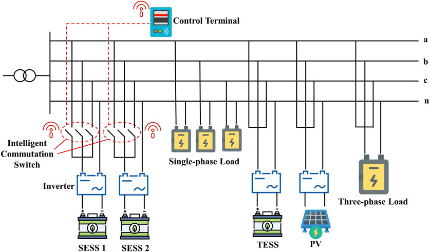
Figure 1. Three-phase power supply and utilization system structure of public building.

The SESS phase selection system consists of SESS, intelligent commutation switch, and control terminal. Assuming that the monitoring terminal detects the distribution of three-phase injection power is $P_a>P_b>P_c$ at a certain moment. According to the requirements of the power supply and utilization system for load unbalance degree, the control terminal will control the commutation switch to discharge SESS 1 to a-phase. At the same time, SESS 2 will be controlled to charge c-phase. While achieving three-phase unbalance management, SESSs can also be jointly scheduled with TESS to further improve the PV consumption rate.

3 Typical power supply-demand mode selection method based on multivariate time series clustering

Considering the correlation between the internal load operation and the external lighting and temperature of public buildings, a spatial weighted matrix distance-based affinity-propagation (SWMDAP) clustering algorithm is proposed to extract typical power supply-demand modes.

SWMDAP algorithm utilizes information granules to represent time series, transforming high-dimensional, fine-grained complex time series into low-dimensional, coarse-grained information granule series. By introducing SWMD to reflect the position information of each element in multivariate time series (MTS), the correlation between variables such as single-phase/three-phase load power and PV output can be quantified, thereby improving the quality of clustering. The specific process of typical mode selection based on the SWMDAP algorithm is shown in Figure 2.

Figure 2

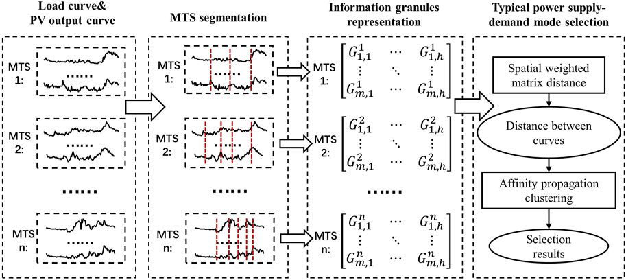
Figure 2. Typical power supply-demand mode selection based on SWMDAP algorithm.

3.1 Multi-granularity interval information granules representation of MTS

Multiple types of data such as PV output and load power are measured at the same time intervals and generated sequentially, which can be expressed as MTS groups. During the 1-year data monitoring period, the daily collection results of data can generally be represented as an MTS. Assume that a MTS is a finite set of M-dimensional vectors observed at time $t_1,t_2,\dots ,t_n$ corresponding to a certain observation day, which can be defined as $D=\left\{\left.X_t={\left[x_{1,t},x_{2,t},\dots ,x_{M,t}\right]}^T\right|1\le t\le N\right\}$. When $M=1$, a MTS becomes a univariate time series. A MTS can be represented by a $M\times N$ matrix, which is expressed as Eq. 1.

$D=\left[X_1,X_2,\dots ,X_N\right]=\left[\left[\begin{array}{c}{x}_{1,1}\\ x_{2,1}\\ ⋮\\ x_{M,1}\end{array}\right]\left[\begin{array}{c}{x}_{1,2}\\ x_{2,2}\\ ⋮\\ x_{M,2}\end{array}\right]\cdots \left[\begin{array}{c}{x}_{1,N}\\ x_{2,N}\\ ⋮\\ x_{M,N}\end{array}\right]\right]=\left[\begin{array}{cccc}{x}_{1,1}& x_{1,2}& \cdots & x_{1,N}\\ x_{2,1}& x_{2,2}& \cdots & x_{2,N}\\ ⋮& ⋮& \ddots & ⋮\\ x_{M,1}& x_{M,2}& \dots & x_{M,N}\end{array}\right](1)$

The multi-granularity interval information granules representation of MTS includes two steps: MTS subsection and information granules representation. To achieve the MTS subsection, it is necessary to establish a cost function that can reflect the internal homogeneity of the subsequences. Then, the cost function is used as an indicator for subsection, so that the internal homogeneity of the segmented subsequences is high while the inter subsequence homogeneity is low. Assuming that a MTS is divided into K segments during the segmentation process, for the kth $\left(1\le k\le K\right)$ subsequence $D_k=\left\{\left.X_t={\left[x_{1,t},x_{2,t},\cdots ,x_{M,t}\right]}^T\right|t_a\le t\le t_b\right\}$ ($t_a$ and $t_b$, respectively represent the starting and ending observation times of the subsequence $D_k$), this paper defines the cost function $S_k$ as Eq. 2.

$S_k=\sum _{m=1}^M{E}_{m,k}=\sum _{m=1}^M\sum _{t=t_a}^{t_b}{\left(x_{m,t}-k_{m,k}t-b_{m,k}\right)}^2(2)$

where, $E_{m,k}$ is the fitting error of the mth variable dimension in subsequence $D_k$. $b_{m,k}$ and $k_{m,k}$ are the linear function constant term and first-order regression coefficient fitted by the least squares method for the subsegment of the mth variable dimension in subsequence $D_k$.

Furthermore, with the goal of minimizing the sum of each subsequence’s cost function values, a segmentation algorithm is used to obtain the optimal partitioning of the time series. For piecewise linear approximation, Keogh and Pazzani (1999) point out that bottom-up segmentation can achieve the best results without the need for real-time segmentation. Therefore, this paper uses the bottom-up segmentation method to complete MTS segmentation. This segmentation method first creates the best-fitting straight lines for the MTS D, which generates N/2 subsequences. Then, the cost function value of each adjacent subsequence after merging is calculated. Among all adjacent subsequences, the adjacent subsequence with the lowest cost function value after merging is selected and merged. Finally, iterate continuously until the number of segments in the sequence reaches a predetermined value.

Divide D into H non-overlapping and continuous subsequences $\left\{D_1,D_2,\cdots ,D_H\right\}$ through time series segmentation. Assuming that the hth subsequence of the mth variable dimension $D_{m,h}\left(m\in M,h\in H\right)$ is fitted with a straight line to obtain regression coefficient $k_{m,h}$, constant term $b_{m,h}$, and residual term $U_{m,h}$. Therefore, the information granule of $D_{m,h}$ can be initially represented as $G_{m,h}=\left\{k_{m,h},b_{m,h},U_{m,h}\right\}$. If the subsequence $D_{m,h}$ contains L observation data points after segmentation, then $U_{m,h}=\left\{u_{m,1},u_{m,2},\cdots ,u_{m,L}\right\}$. According to Cramer decomposition theory, the variation of residual term is a process that tends towards stability. Therefore, by using the interval set to represent residual sequence $U_{m,h}$, information granule $G_{m,h}$ can be further simplified.

According to the reasonable granularity principle, the optimal interval is represented by the composite product of coverage index and specificity index. Select the average value $rep\left(U_{m,h}\right)$ of the sequence $U_{m,h}$ as a numerical representation, the data can be divided into two parts from the middle. Finally, the interval boundary functions $V\left({\mathrm{\Omega }}^U\right)$ and $V\left({\mathrm{\Omega }}^L\right)$ of the upper and lower bounds are represented as Eqs 3, 4.

$V\left({\mathrm{\Omega }}^U\right)=f_1\left(card\left(x\in U_{m,h}|rep\left(U_{m,h}\right)<x\le {\mathrm{\Omega }}^U\right)\right)\times f_2\left(\left|{\mathrm{\Omega }}^U-rep\left(U_{m,h}\right)\right|\right)(3)$

$V\left({\mathrm{\Omega }}^L\right)=f_1\left(card\left(x\in U_{m,h}|{\mathrm{\Omega }}^L\le x<rep\left(U_{m,h}\right)\right)\right)\times f_2\left(\left|rep\left(U_{m,h}\right)-{\mathrm{\Omega }}^L\right|\right)(4)$

Where, $card\left(x\in U|a<x\le b\right)$ represents the number of elements belonging to sequence U within the range of $\left(a,\left.b\right]\right.$. $f_1$ and $f_2$ are optional functions that can effectively control the impact of specificity and coverage on interval construction, which can be expressed as Eqs 5, 6.

$f_1\left(u\right)=u(5)$

$f_2\left(u\right)=\mathit{exp}\left(-\alpha u\right)(6)$

Where, α indicates the information granularity level, $\alpha \ge 0$. By changing α, the “coverage” and “specificity” of the information granule can be controlled.

When $V\left({\mathrm{\Omega }}^U\right)$ and $V\left({\mathrm{\Omega }}^L\right)$ take the maximum values respectively, the optimal interval $\left[{\mathrm{\Omega }}_{m,h}^{L,\alpha },{\mathrm{\Omega }}_{m,h}^{U,\alpha }\right]$ that characterizes the residual sequence $U_{m,h}$ under parameter α can be obtained through Eqs 7, 8:

${\mathrm{\Omega }}_{m,h}^{U,\alpha }=\underset{{\mathrm{\Omega }}^U\ge rep\left(U_{m,h}\right)}{\mathrm{argmax}}V\left({\mathrm{\Omega }}^U\right)(7)$

${\mathrm{\Omega }}_{m,h}^{L,\alpha }=\underset{{\mathrm{\Omega }}^L\le rep\left(U_{m,h}\right)}{\mathrm{argmax}}V\left({\mathrm{\Omega }}^L\right)(8)$

Finally, the residual sequence $U_{m,h}$ can be represented by the interval set. Obviously, using a single interval set to construct the information granule is quite limited. To ensure that the information granule can fully retain the characteristics of MTS, this paper adopts interval sets under three different α to represent the residual sequence. Considering that residual can be attached to the constant term, the information general of $D_{m,h}$ can be further represented as Eq. 9:

$G_{m,h}=\left\{k_{m,h},{\mathrm{\Omega }}_{m,h}=\left\{\left[b_{m,h}+{\mathrm{\Omega }}_{m,h}^{L,\alpha 1},b_{m,h}+{\mathrm{\Omega }}_{m,h}^{U,\alpha 1}\right],\left[b_{m,h}+{\mathrm{\Omega }}_{m,h}^{L,\alpha 2},b_{m,h}+{\mathrm{\Omega }}_{m,h}^{U,\alpha 2}\right],\right.\right.$

$\left.\left.\left[b_{m,h}+{\mathrm{\Omega }}_{m,h}^{L,\alpha 3},b_{m,h}+{\mathrm{\Omega }}_{m,h}^{U,\alpha 3}\right]\right\}\right\}(9)$

Where, the interval coverage under α1 is the highest. The interval specificity and coverage under α2 are at a moderate level. The interval specificity under α3 is the highest. Finally, the residual term and constant term are merged to obtain a simplified information general representation of $D_{m,h}$: $G_{m,h}=\left\{k_{m,h},{\mathrm{\Omega }}_{m,h}=\left\{\left[a_{m,h}^{\alpha 1},b_{m,h}^{\alpha 1}\right],\left[a_{m,h}^{\alpha 2},b_{m,h}^{\alpha 2}\right],\left[a_{m,h}^{\alpha 3},b_{m,h}^{\alpha 3}\right]\right\}\right\}$.

Therefore, the time series $D=\left\{D_1,D_2,\cdots ,D_H\right\}$ can be expressed as a $M\times H$ dimensional “information granules matrix” G, which is shown as Eq. 10.

$G=\left[G_1,G_2,\cdots ,G_H\right]=\left[\left[\begin{array}{c}{G}_{1,1}\\ G_{2,1}\\ ⋮\\ G_{M,1}\end{array}\right],\left[\begin{array}{c}{G}_{1,2}\\ G_{2,2}\\ ⋮\\ G_{M,2}\end{array}\right],\cdots ,\left[\begin{array}{c}{G}_{1,H}\\ G_{2,H}\\ ⋮\\ G_{M,H}\end{array}\right]\right]=\left[\begin{array}{cccc}{G}_{1,1}& G_{1,2}& \cdots & G_{1,H}\\ G_{2,1}& G_{2,2}& \cdots & G_{2,H}\\ ⋮& ⋮& \ddots & ⋮\\ G_{M,1}& G_{M,2}& \dots & G_{M,H}\end{array}\right](10)$

3.2 Spatially weighted matrix distance extraction

To calculate the MTS distance, this paper adopts an MTS similarity measurement method proposed in the ref. He and Tan (2018): SWMD.

Assume that MTS $D^i$, $D^j$ of observation day i and j are expressed as $M\times H$ dimensional information granules matrix $G^i$ and $G^j$. For the convenience of matrix calculation, this paper changes $G^i$, $G^j$ from an $M\times H$ feature matrix to a $1\times \left(M\times H\right)$ feature matrix $g^i$, $g^j$, which is represented as Eqs 11, 12.

$G^i\to g^i=\left[G_{1,1}^i,G_{2,1}^i,\dots ,G_{M,1}^i,G_{1,2}^i,G_{2,2}^i,\dots ,G_{M,2}^i,\dots ,G_{1,H}^i,G_{2,H}^i,\dots ,G_{M,H}^i\right]=\left[g_1^i,g_2^i,\dots ,g_{M\times H}^i\right](11)$

$G^j\to g^j=\left[G_{1,1}^j,G_{2,1}^j,\dots ,G_{M,1}^j,G_{1,2}^j,G_{2,2}^j,\dots ,G_{M,2}^j,\dots ,G_{1,H}^j,G_{2,H}^j,\dots ,G_{M,H}^j\right]=\left[g_1^j,g_2^j,\dots ,g_{M\times H}^j\right](12)$

Where, assuming $g_u^i$ is the uth element of the information granules matrix $g^i$, corresponding to $G_{a,b}^i$, whose position is row a and column b in $G^i$. Then, u satisfies $u=a+M\times \left(b-1\right)$.

Then, the SWMD between $G^i$ and $G^j$ can be expressed as Eq. 13.

$SWMD\left(G^i,G^j\right)=\sqrt{\sum _{u,v=1}^{M\times H}{s}_{uv}d\left(g_u^i,g_u^j\right)d\left(g_v^i,g_v^j\right)}(13)$

Where, $d\left(\bullet ,\bullet \right)$ is the distance between pairs of information granules. $s_{uv}$ is the spatial weighted matrix coefficient corresponding to $d\left(g_u^i,g_u^j\right)$ and $d\left(g_v^i,g_v^j\right)$.

Assume that there are two information granules $g_1$, $g_2$. The distance $d\left(g_1,g_2\right)$ between $g_1$ and $g_2$ can be calculated as Eq. 14.

$d\left(g_1,g_2\right)=d_{\mathrm{\Omega }}+d_{trend}=\sqrt{\begin{array}{c}{\left(a_2^{\alpha 1}-a_1^{\alpha 1}\right)}^2+{\left(a_2^{\alpha 2}-a_1^{\alpha 2}\right)}^2+{\left(a_2^{\alpha 3}-a_1^{\alpha 3}\right)}^2\\ {+\left(b_2^{\alpha 1}-b_1^{\alpha 1}\right)}^2+{\left(b_2^{\alpha 2}-b_1^{\alpha 2}\right)}^2+{\left(b_2^{\alpha 3}-b_1^{\alpha 3}\right)}^2\end{array}}+\eta \left|k_1-k_2\right|(14)$

Where, $g_1:\left\{k_1,{\mathrm{\Omega }}_1=\left\{\left[a_1^{\alpha 1},b_1^{\alpha 1}\right],\left[a_1^{\alpha 2},b_1^{\alpha 2}\right],\left[a_1^{\alpha 3},b_1^{\alpha 3}\right]\right\}\right\}$, $g_2:\left\{k_2,{\mathrm{\Omega }}_2=\left\{\left[a_2^{\alpha 1},b_2^{\alpha 1}\right],\left[a_2^{\alpha 2},b_2^{\alpha 2}\right],\left[a_2^{\alpha 3},b_2^{\alpha 3}\right]\right\}\right.$. $d_{\mathrm{\Omega }}$ is the distance between the interval set of information granules $g_1$ and $g_2$. $d_{trend}$ is the distance between the trend items $k_1$ and $k_2$. η is the correction parameter.

The calculation formula for the spatial weighting matrix coefficient $s_{uv}$ is as Eq. 15.

$s_{uv}=\frac{1}{2\pi {\left(1-h^{-1}\right)}^2}\mathit{exp}\left(-\frac{d_{D,uv}}{2{\left(1-h^{-1}\right)}^2}\right)(15)$

Where, if the position of $g_u^i$, $g_u^j$ is the row a and column b in $G^i$, $G^j$, the position of $g_v^i$, $g_v^j$ is row $a^{\prime }$ and column $b^{\prime }$ in $G^i$, $G^j$, then $d_{D,uv}=\sqrt{{\left(a-a^{\prime }\right)}^2+{\left(b-b^{\prime }\right)}^2}$.

3.3 Affinity propagation clustering based on spatially weighted matrix distance

Affinity propagation (AP) algorithm is a clustering algorithm that simulates information propagation (Frey and Dueck, 2007). AP algorithm treats each sequence as a data point and takes the similarity between pairs of data points as input. Then, cluster information is continuously exchanged between data points until high-quality clustering results appear. AP algorithm mainly consists of two parts: initialization and message exchanged.

The initialization of the AP algorithm requires the input of the similarity matrix S of the data to be clustered. The off-diagonal element $s\left(i,j\right)$ in the similarity matrix represents the similarity between data point i and j. The diagonal element $s\left(i,i\right)$ in the similarity matrix is the bias parameter p (preference), which is pre-set by the user. The bias parameter value of each data point is generally the same, which is set as the median of the similarity matrix. The larger the bias parameter value, the more likely data point i is to become the cluster center.

Traditional AP clustering adopts negative Euclidean distance to form similarity, which has difficulties when dealing with multi-variable clustering. Therefore, this paper adopts SWMD to replace Euclidean distance. Meanwhile, the bias parameter value p on the similarity matrix S of traditional AP clustering is the same, which means the same probability of all data points being selected as representative points. However, this ignores the structural information of the data itself. If there are more points around a point within a cluster, the probability of that point being the center of the cluster should be higher. So the idea of density clustering can be introduced, using the density of data points around a point to set the bias parameter value for that point. Therefore, the modified similarity matrix is expressed as Eq. 16.

$s\left(i,j\right)=\left\{\begin{array}{l}-SWMD{\left(x_i,x_j\right)}^2,i\ne j\\ -n\epsilon /m_i,i=j\end{array}\right.(16)$

Where, n is the number of data points. $m_i$ is the number of data points within the neighborhood of point i. ε is the median of similarities between data points.

The message exchanged of the AP algorithm mainly includes the “responsibility” $r\left(i,k\right)$ and the “availability” $a\left(i,k\right)$. $r\left(i,k\right)$ reflects the accumulated evidence for how well-suited point k is to serve as the exemplar for point i, taking into account other potential exemplars for point i. $a\left(i,k\right)$ reflects the accumulated evidence for how appropriate it would be for point i to choose point k as its exemplar, taking into account the support from other points that point k should be an exemplar.

Initially, the “responsibility” r and “availability” a of each data point are both zero. AP algorithm updates the r and a of each point through an iterative formula. Finally, while generating cluster centers, data points will be divided into different clusters. During the iterative process of AP clustering, if the information of each data point changes too much, it may lead to non-convergence of the results. Therefore, a damping factor λ is generally set during iteration to reduce changes in the “responsibility” and “availability”. The formula for the tth iteration is expressed as Eqs 17, 18.

$r^t\left(i,k\right)=\left(1-\lambda \right)\times \left(s\left(i,k\right)-\underset{k^{\prime }\ne k}{\max }\left\{a^{t-1}\left(i,k^{\prime }\right)+s\left(i,k^{\prime }\right)\right\}\right)+\lambda \times r^{t-1}\left(i,k\right)(17)$

$a^t\left(i,k\right)=\left\{\begin{array}{l}\left(1-\lambda \right)\times \left(\min \left\{0,r^{t-1}\left(k,k\right)+\sum _{i^{\prime }\notin \left\{i,k\right\}}\max \left\{0,r^{t-1}\left(i^{\prime },k\right)\right\}\right\}\right)+\lambda \times a^{t-1}\left(i,k\right),i\ne k\\ \left(1-\lambda \right)\times \left(\sum _{i^{\prime }\ne k}\max \left\{0,r^{t-1}\left(i^{\prime },k\right)\right\}\right)+\lambda \times a^{t-1}\left(i,k\right),i=k\end{array}\right.(18)$

When the cluster centers to which all data points belong no longer change, or the changes in the information r and a exchanged by each point are lower than a certain fixed threshold, the iteration stops and the clustering results are output.

Assuming that typical power supply-demand modes need to be extracted from PV and load data of N observation days, the specific process of SWMDAP clustering is as follows.

1) Divide MTS $D^n\left(n=1,2,\cdots ,N\right)$ of each observation day into H segments by the bottom-up segmentation method.

2) Use the information granule representation method to construct the “information granules matrix” $G^n$ corresponding to $D^n$.

3) Calculate the SWMD between $G^n\left(n=1,2,\cdots ,N\right)$ by Eq. 13.

4) Obtain the similarity matrix by Eq. 16.

5) Initialize the “availability” $a^{\left(0\right)}\left(i,k\right)=0$ and “responsibility” $r^{\left(0\right)}\left(i,k\right)=0$ of data points. And set the damping factor λ.

6) Update $a^{\left(t\right)}\left(i,k\right)$ and $r^{\left(t\right)}\left(i,k\right)$ for the tth iteration by Eqs 17, 18. And update the clustering centers for each MTS.

7) Determine the condition for stopping the iteration. If the condition is met, output the clustering result; otherwise, return to 6).

4 Energy storage system capacity planning for public building

This chapter models the capacity configuration problem of SESS and TESS in the public building. Based on the time scale differences between capacity configuration and optimized operation, a bi-level optimization model is constructed. The transfer relationship of optimization decision variables between upper and lower levels is shown in Figure 3. Firstly, the upper level transfers the planned capacity of SESS and TESS to the lower-level model. The lower level simulates the operation of ESS based on the given capacity. Then the optimal cost of electricity purchasing and light discarding will be returned to the upper-level model. Secondly, the upper-level model modifies the life cycle cost based on lower-level results and further optimizes the planned capacity of SESS and TESS. Finally, through optimization iterations between upper and lower levels, the optimal ESS configuration and operation plan will be obtained with the minimum life cycle cost within the planning period.

Figure 3

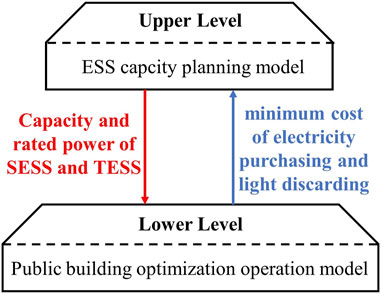
Figure 3. Transfer relationship of optimization variables between upper and lower levels.

Among them, the upper-level model aims at minimizing the life cycle cost on a long time scale to determine the capacity and rated power of SESS and TESS. The lower-level model aims at minimizing all-weather operating costs on a short time scale to optimize the switching strategy of the commutation switch and ESS charging/discharging strategy.

4.1 Upper-level capacity planning model

The current cost of ESS in the initial investment process is still high, making it difficult to achieve positive returns in the short term. Therefore, it will be more meaningful to consider the revenue and cost of ESS throughout its life cycle on a long-term scale. The core concept of life cycle cost refers to the total sum of all direct and indirect expenses incurred during the production, operation, maintenance, and premium recovery stages. Life cycle cost technology has been applied in many aspects such as power grid planning and power system asset management.

4.1.1 Objective function

The upper-level capacity planning model aims at minimizing the net present value of the life cycle cost. The objective function can be expressed as Eq. 19.

$\min C^{total}=C^{inv}+C^{main}+C^{grid}+C^{cut}(19)$

Where, $C^{total}$ is the net present value of the life cycle cost. $C^{inv}$, $C^{main}$, $C^{grid}$, and $C^{cut}$ represent the costs of initial investment, operation and maintenance, electricity purchase, and PV curtailment penalty, respectively.

The initial investment cost of ESS can be expressed as Eq. 20.

$C^{inv}=\left(\sum _{k=1}^2{E}^{s,k,Ebat}+E^{t,Ebat}\right)e^{inv,Ebat}+\left(\sum _{k=1}^2{E}^{s,k,Pbat}+E^{t,Pbat}\right)e^{inv,Pbat}(20)$

Where, $E^{s,k,Ebat}$, $E^{t,Ebat}$ represent the rated capacity for the initial installation of SESS k and TESS, respectively. $E^{s,k,Pbat}$, $E^{t,Pbat}$ represent the rated power for the initial installation of SESS k and TESS, respectively. $e^{inv,Ebat}$, $e^{inv,Pbat}$ represent the ESS cost per unit capacity and power, respectively.

The operation and maintenance cost of ESS can be expressed as Eq. 21.

$C^{main}=\sum _{n=1}^{N^Y}\frac{\left(\sum _{k=1}^2{E}^{s,k,Ebat}+E^{t,Ebat}\right)e^{main,Ebat}+\left(\sum _{k=1}^2{E}^{s,k,Pbat}+E^{t,Pbat}\right)e^{main,Pbat}}{{\left(1+r\right)}^{n-1}}(21)$

Where, $e^{main,Pbat}$, $e^{main,Ebat}$ respresent the operating cost coefficient of unit energy storage power and installation capacity, respectively. r is the discount rate. $N^Y$ is the planning cycle.

When the electricity supply of PV cannot meet the load demand, electricity needs to be purchased from the power grid. The electricity purchase cost can be expressed as Eq. 22.

$C^{grid}=\sum _{n=1}^{N^Y}\left[\frac{1}{{\left(1+r\right)}^{n-1}}\sum _{t=1}^{T^Y}{\lambda }_t^{grid}{P}_t^{grid}\Delta t\right](22)$

Where, $P_t^{grid}$, ${\lambda }_t^{grid}$ represent the power purchased from the power grid and the corresponding electricity purchase price at time period t, respectively. Δt is the time interval. $T^Y$ is the number of time periods throughout the year.

In order to promote the local consumption of PV, the curtailment of PV should be included in the cost, which can be expressed as Eq. 23.

$C^{cut}=\sum _{n=1}^{N^Y}\left[\frac{1}{{\left(1+r\right)}^{n-1}}\sum _{t=1}^{T^Y}{\lambda }^{cut}{P}_t^{pv,cut}\Delta t\right](23)$

Where, ${\lambda }^{cut}$ is the unit solar power curtailment penalty cost. $P_t^{pv,cut}$ is the amount of solar power curtailment at time period t.

4.1.2 Constraints

The capacity of ESS is proportional to the rated power, which can be expressed as Eqs 24, 25.

$E^{s,k,Ebat}={\beta }^{bat}{E}^{s,k,Pbat}(24)$

$E^{t,Ebat}={\beta }^{bat}{E}^{t,Pbat}(25)$

Where, ${\beta }^{bat}$ is the energy multiplier of ESS.

4.2 Lower-level optimization operation model

On the basis of general economic operation problems, the lower-level optimization operation model additionally considers the PV consumption rate and three-phase unbalance problem of the building. Combined with the relevant constraints during operation, the optimization of switching and charging/discharging strategies can be ultimately achieved.

4.2.1 Objective function

Integrating the electricity purchase cost and PV curtailment cost, the lower-level optimization operation model aims at minimizing the all-day operation cost of the public building. The objective function can be expressed as Eq. 26.

$\min C^{oper}=\sum _{t=1}^{T^D}\left({\lambda }_t^{grid}{P}_t^{grid}\Delta t+{\lambda }^{cut}{P}_t^{pv,cut}\Delta t\right)(26)$

Where, $C^{oper}$ is the all-day operation cost of the public building. $T^D$ is the number of daily operating time periods.

4.2.2 Constraints

The power balance constraint of the public building can be expressed as Eq. 27.

$P_{abc,t}^{load}+P_{abc,t}^{bat,ch}+\sum _{\phi \in \left\{a,b,c\right\}}\left(\sum _{k=1}^2{P}_{\phi ,t}^{bat,k,ch}+P_{\phi ,t}^{load}\right)=P_t^{pv}+P_t^{grid}+P_{abc,t}^{bat,dis}+\sum _{\phi \in \left\{a,b,c\right\}}{\displaystyle \sum _{k=1}^2}{P}_{\phi ,t}^{bat,k,dis}(27)$

Where, $P_{abc,t}^{load}$, $P_{abc,t}^{bat,ch}$, $P_{abc,t}^{bat,dis}$ represent the three-phase load power, TESS charging power and discharge power at time period t, respectively. $P_{\phi ,t}^{load}$, $P_{\phi ,t}^{bat,k,ch}$, $P_{\phi ,t}^{bat,k,dis}$ represent the φ-phase load power, φ-phase charging power and discharge power of SESS k at time period t, respectively. $P_t^{pv}$ is the actual dispatched output of PV at time period t.

The actual dispatched PV output of the public building should not exceed the PV output power. Therefore, the PV curtailment power constraint can be expressed as Eqs 28, 29.

$P_t^{pv,cut}=P_t^{pv,c}-P_t^{pv}(28)$

$0\le P_t^{pv}\le P_t^{pv,c}(29)$

Where, $P_t^{pv,c}$ is the output power of PV at time period t.

SESS is equipped with a commutation switch, which can only be connected to one phase of the three-phase lines at each time period. Therefore, the charging and discharging power constraints of SESS k can be expressed as Eqs 30, 31.

$\sum _{\phi \in \left\{a,b,c\right\}}{u}_{\phi ,t}^{bat,k,ch}+\sum _{\phi \in \left\{a,b,c\right\}}{u}_{\phi ,t}^{bat,k,dis}\le 1(30)$

$\left\{\begin{array}{c}0\le P_{\phi ,t}^{bat,k,ch}\le u_{\phi ,t}^{bat,k,ch}{E}^{s,k,Pbat}\\ 0\le P_{\phi ,t}^{bat,k,dis}\le u_{\phi ,t}^{bat,k,dis}{E}^{s,k,Pbat}\end{array}\right.,\phi \in \left\{a,b,c\right\}(31)$

Where, $u_{\phi ,t}^{bat,k,ch}$, $u_{\phi ,t}^{bat,k,dis}$ represent the charging and discharging status of SESS k at time period t, both of which are binary variables. $u_{\phi ,t}^{bat,k,ch}=1$ or $u_{\phi ,t}^{bat,k,dis}=1$ represent that SESS k is connected to the φ-phase and in the charging/discharging state at time period t.

The state-of-charge (SOC) constraints of SESS k are expressed as Eqs 32–34.

${SOC}_t^{bat,s,k}={SOC}_{t-1}^{bat,s,k}+\sum _{\phi \in \left\{a,b,c\right\}}\left(\frac{P_{\phi ,t}^{bat,k,ch}{\eta }^{ch}\Delta t}{E^{s,k,Ebat}}-\frac{P_{\phi ,t}^{bat,k,dis}\Delta t}{{{\eta }^{dis}E}^{s,k,Ebat}}\right)(32)$

${SOC}^{bat,s,\mathit{min}}\le {SOC}_t^{bat,s,k}\le {SOC}^{bat,s,\mathit{max}}(33)$

${SOC}_T^{bat,s,k}={SOC}_0^{bat,s,k}(34)$

Where, ${SOC}_t^{bat,s,k}$ is the SOC of SESS k at time period t. ${\eta }^{ch}$, ${\eta }^{dis}$ represent the charging and discharging efficiency of ESS, respectively. ${SOC}^{bat,s,\mathit{min}}$, ${SOC}^{bat,s,\mathit{max}}$ represent the minimum and maximum SOC of SESS, respectively.

The charging and discharging power constraints of TESS are expressed as Eqs 35, 36.

$u_{abc,t}^{bat,ch}+u_{abc,t}^{bat,dis}\le 1(35)$

$\left\{\begin{array}{l}0\le P_{abc,t}^{bat,ch}\le u_{abc,t}^{bat,ch}{E}^{t,Pbat}\\ 0\le P_{abc,t}^{bat,dis}\le u_{abc,t}^{bat,dis}{E}^{t,Pbat}\end{array}\right.(36)$

Where, $u_{abc,t}^{bat,ch}$, $u_{abc,t}^{bat,dis}$ represent the charging and discharging status of TESS at time period t, both of which are binary variables. $u_{abc,t}^{bat,ch}=1$ or $u_{abc,t}^{bat,dis}=1$ represents that TESS is in the charging/discharging state at time period t. $P_{abc,t}^{bat,ch}$, $P_{abc,t}^{bat,dis}$ represent the charging and discharging power of TESS at time period t, respectively.

The SOC constraints of TESS are expressed as Eqs 37–39.

${SOC}_t^{bat,t}={SOC}_{t-1}^{bat,t}+\frac{P_{abc,t}^{bat,ch}{\eta }^{ch}\Delta t}{E^{t,Ebat}}-\frac{P_{abc,t}^{bat,dis}\Delta t}{{\eta }^{dis}{E}^{t,Ebat}}(37)$

${SOC}^{bat,t,\mathit{min}}\le {SOC}_t^{bat,t}\le {SOC}^{bat,t,\mathit{max}}(38)$

${SOC}_T^{bat,t}={SOC}_0^{bat,t}(39)$

Where, ${SOC}_t^{bat,t}$ is the SOC of TESS at time period t. ${SOC}^{bat,t,\mathit{min}}$, ${SOC}^{bat,t,\mathit{max}}$ represent the minimum and maximum SOC of TESS, respectively.

Due to the complexity of commonly used formulas for calculating the voltage or current’s three-phase unbalance degree, it is difficult to express them concisely in the model of this paper. According to the ref. Zhan et al. (2015), this paper uses the three-phase unbalance degree of the load to approximately represent the voltage or current. In this paper, the three-phase unbalance constraints are expressed as Eqs 40–42.

${\varphi }_t^{unb}=\frac{3\bullet \max \left\{\left|P_{a,t}-P_t^{avg}\right|,\left|P_{b,t}-P_t^{avg}\right|,\left|P_{c,t}-P_t^{avg}\right|\right\}}{{\displaystyle \sum _{\phi \in \left\{a,b,c\right\}}}{P}_{\phi ,t}^{load}}\le {\delta }^{unb}(40)$

$P_t^{avg}=\frac{1}{3}\left(P_{a,t}+P_{b,t}+P_{c,t}\right)(41)$

$P_{\phi ,t}=P_{\phi ,t}^{load}+\sum _{k=1}^2\left(P_{\phi ,t}^{bat,k,ch}-P_{\phi ,t}^{bat,k,dis}\right),\phi \in \left\{a,b,c\right\}(42)$

Where, ${\varphi }_t^{unb}$ is three-phase unbalance degree at time period t. ${\delta }^{unb}$ is the allowable upper limit of three-phase unbalance degree. $P_{\phi ,t}$ is the φ-phase injected active power at time period t. $P_t^{avg}$ is the average value of the active power injected into the three phases at time period t.

5 Bi-level optimization model solution method

The typical power supply-demand mode selection method greatly reduces the computational complexity of the lower-level optimization operation model. Then the efficiency of model optimization can be improved. Therefore, based on the typical mode extraction results, the solution process of the bi-level optimization model is shown in Figure 4. Compared to traditional genetic algorithm, elitist genetic algorithm (EGA) incorporate an elite preservation strategy, which copies the individual with the highest fitness value during the population evolution process directly to the next-generation population without undergoing crossover, mutation, and other operations. This avoids the disruption of the optimal individual during the evolution process. EGA has the advantages of global convergence and fast convergence speed. Therefore, this paper uses EGA and Gurobi solver to solve the bi-level optimization model.

Figure 4

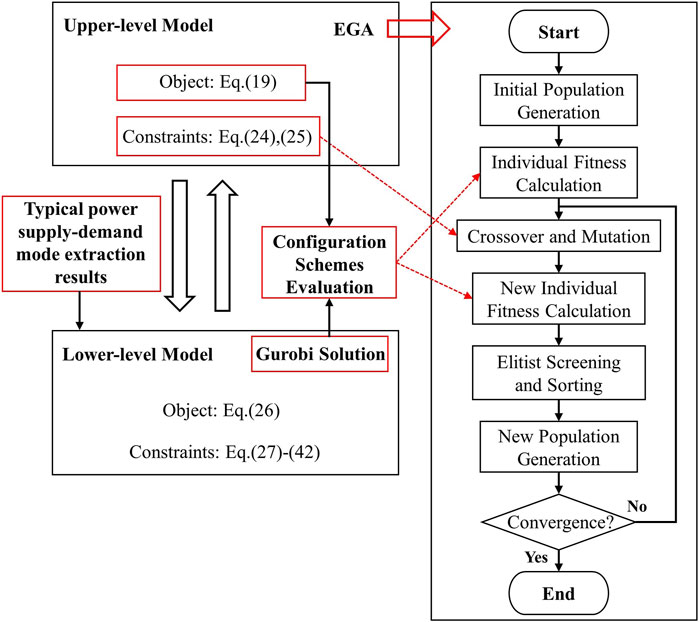
Figure 4. The solution process of the Bi-level optimization model.

EGA is adopted to randomly generate the capacity configuration schemes of SESS and TESS in the upper-level capacity planning model. The lower-level optimization operation model determines the optimal typical mode dispatching plan under this capacity configuration through mixed-integer linear programming. During the interaction process, the lower level returns the optimal typical mode dispatching results to the upper level for evaluation of individual fitness. On this basis, the upper level aims to minimize the life cycle cost and update the capacity of SESS and TESS through selection, crossover, and mutation. The iterative process is repeated until the algorithm converges. Finally, the public building energy storage optimal planning scheme will be obtained.

6 Case study

6.1 Case setting

Historical measured data of PV and load in a large public building is adopted in this paper. With a 10-year operational planning, the ESS capacity configuration and operational optimization will be finished. Among them, the building is equipped with a total capacity of 700 kW PV panels. The PV and load curves obtained with a sampling time interval of 1 h are shown in Figure 5. Due to relevant policy restrictions, public buildings are not allowed to return electricity to the grid.

Figure 5

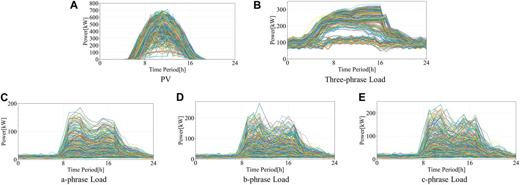
Figure 5. Historical measured data of PV and load in the public building. (A): PV, (B): Three-phase load, (C): a-phase load, (D): b-phase load, (E): c-phase load.

The SESS and TESS are composed of the same type of battery, and the relevant physical and economic parameters are shown in Table 1, respectively. The initial SOC of the ESS ${SOC}_0^{bat,s,k}={SOC}_0^{bat,t}=0.2$. Energy multiplier ${\beta }^{bat}=8$. In the calculation process of the life cycle cost, the discount rate $r=0.08$. The unit solar power curtailment penalty cost ${\lambda }^{cut}=0.6$ RMB/kWh. Time-of-use electricity prices are shown in Table 2. The allowable upper limit of the three-phase unbalance degree ${\delta }^{unb}=0.12$.

Table 1

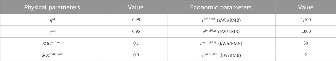
Table 1. Physical and economic parameters of ESS.

Table 2

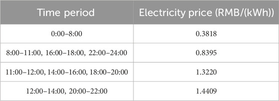
Table 2. Time-of-use electricity price.

Typical power supply-demand mode selection is achieved by using the SWMDAP algorithm. The SWMDAP algorithm adopts the method described in the ref. Frey and Dueck (2007) to set the bias parameter p and damping factor λ. Among them, p takes the median of the similarity matrix, and λ takes the default value of 0.9.

To verify the effectiveness of the proposed typical mode selection method in the planning scenario of this paper, the typical mode selection method based on the SWMDAP clustering algorithm was compared with three clustering algorithms, including AP clustering, K-means, and hierarchical clustering.

Meanwhile, in order to further verify the feasibility of SESS and TESS joint dispatch in PV local consumption and three-phase unbalance management, this paper sets up the following four cases for comparison, as shown in Table 3.

Table 3

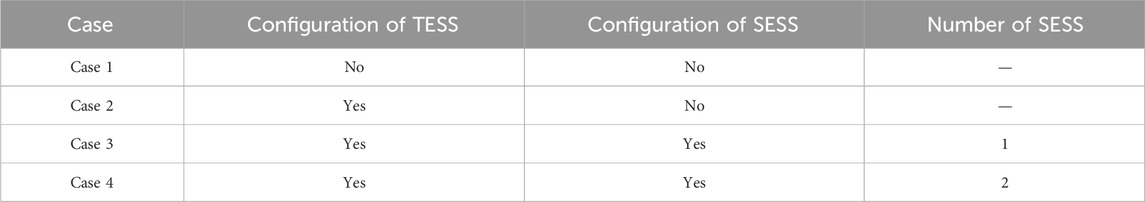
Table 3. Case setting.

6.2 Effectiveness analysis of typical power supply-demand mode selection method based on SWMDAP algorithm

For 1 year data of PV and load, the SWMDAP clustering algorithm is adopted to select typical power supply-demand modes. The selection results are shown in Figure 6. Among them, the weight of each typical mode is shown in Table 4.

Figure 6

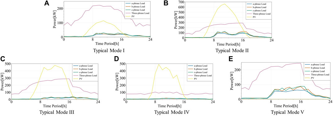
Figure 6. Typical power supply-demand mode selection results. (A): Typical Mode I, (B): Typical Mode II, (C): Typical Mode III, (D): Typical Mode IV, (E): Typical Mode V.

Table 4

Table 4. Weight of each typical power supply-demand mode.

In order to compare with the SWMDAP clustering algorithm, the clustering number of K-means and hierarchical clustering is selected to be 5. Meanwhile, the parameter setting of the AP clustering algorithm is consistent with SWMDAP. Based on the AP clustering algorithm, 24 cluster centers are ultimately obtained, which will not effectively reduce the computational complexity of ESS planning. The typical mode selection results contain various extreme scenarios, but typicality is lacking. Therefore, ESS configuration optimization is carried out based on the typical operational modes obtained from the remaining three algorithms. Finally, the ESS configuration results of the public building based on different typical mode selection methods are shown in Table 5.

Table 5

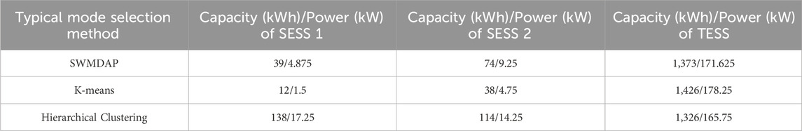
Table 5. Comparison of public building ESS configuration results under different typical mode selection methods.

It can be seen from Table 5 that the SESS capacity configuration result based on the SWMDAP algorithm in this paper is much greater than the result based on the K-means algorithm, which can better manage the three-phase unbalance in the building. However, the typical mode selection method based on the K-means algorithm lacks extreme scenarios similar to Typical Mode II and V. This leads to an overly conservative configuration result of SESS capacity, which cannot effectively cope with some three-phase unbalance situations. Meanwhile, the total configuration capacity of ESS based on the hierarchical clustering is larger than SWMDAP algorithm. This is because hierarchical clustering lacks extreme scenarios similar to Typical Mode I and V. The overly optimistic assessment of PV output makes it easier to recover the investment cost of ESS. On the one hand, the typical mode selection method based on the SWMDAP algorithm can quantify the correlation between different variables’ dimension. Therefore, it can more accurately extract the difference between single-phase loads. On the other hand, the fluctuation differences of multi-dimensional variables can be identified through SWMD, which ensures that clustering results can have both typicality and extremism.

6.3 Effectiveness analysis of SESS equipped with commutation switch for three-phase unbalance management

According to the typical mode selection results based on the SWMDAP algorithm, the ESS configuration results of Case 1∼Case 4 are obtained, which are shown in Table 6. It can be seen from Table 6 that the total capacity of ESSs in Case 3 and Case 4 has increased compared to Case 2. This is because the operation optimization of SESS not only needs to consider the goals of PV local consumption and reducing electricity purchase cost, but also takes into account the three-phase unbalance constraint of Eq. 32. Meanwhile, comparing Case 3 and Case 4, it can be found that the total capacity of SESS is consistent under the two configuration results. However, considering that the coordinated operation of two SESSs makes it easier to achieve the three-phase unbalance constraint compared to a single SESS, Case 4 can correspondingly reduce the capacity configuration of TESS.

Table 6

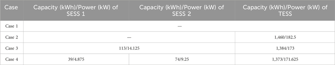
Table 6. ESS Configuration results of Case 1∼Case 4.

The life cycle costs of Case1∼Case4 are shown in Table 7. Compared to Case 1 without ESS, Case 2∼Case 4 significantly reduces the cost of electricity purchase and PV curtailment penalty, and achieves cost recovery for initial investment and maintenance. Due to the addition of the three-phase unbalance constraint, the life cycle cost of Case 3 and Case 4 has increased. Meanwhile, taking advantage of the coordinated operation of two SESSs, Case 4 has lower costs than Case 3 in all four aspects.

Table 7

Table 7. Life cycle cost calculation results of Case 1∼Case 4.

The comparison of three-phase unbalance degree ${\varphi }_t^{unb}$ between Case 2∼Case 4 under five typical modes is shown in Figure 7. Comparing Figures 7A–E, it can be found that configuring SESS has a significant effect on managing three-phase unbalance. Meanwhile, compared to a single SESS, two SESSs will have better three-phase unbalance management effects by discharging at maximum-phase load and charging at minimum-phase load, respectively.

Figure 7

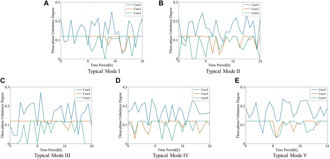
Figure 7. Comparison of three-phase unbalance degree curves between Case 2∼Case 4. (A): Typical Mode I, (B): Typical Mode II, (C): Typical Mode III, (D): Typical Mode IV, (E): Typical Mode V.

6.4 Economic analysis under different upper limits ${\mathit{\delta }}^{\mathit{u}\mathit{n}\mathit{b}}$ of three-phase unbalance degree

Under different values of ${\delta }^{unb}$, the corresponding ESS configuration results and life cycle cost are shown in Table 8. It can be found that when ${\delta }^{unb}$ is within the range of 0.12∼0.08, as the degree of three-phase unbalance management deepens, the cost increases significantly. However, when ${\delta }^{unb}$ ranges from 0.16 to 0.12, the increase in cost with the deepening of management is relatively small. Therefore, this paper selects ${\delta }^{unb}=0.12$ can achieve a good three-phase unbalance management effect while ensuring economic efficiency. Meanwhile, when ${\delta }^{unb}=0.08$, the configuration of a single SESS will not be able to meet the three-phase unbalance constraint. In this case, the ability of SESS to reduce operating costs will be weakened, while the capacity of TESS will increase.

Table 8

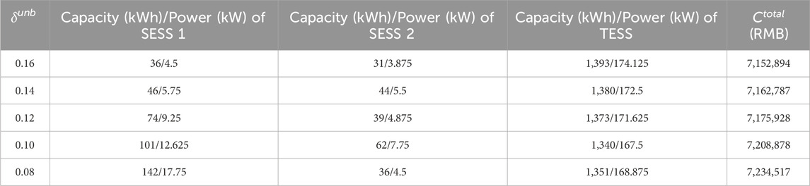
Table 8. ESS Configuration results and life cycle cost under different values of ${\mathit{\delta }}^{\mathit{u}\mathit{n}\mathit{b}}.$

7 Conclusion

In response to the three-phase unbalance problem in large public buildings caused by the temporal differences of electrical load and the connection of single-phase charging piles, this paper proposes an ESS configuration method aimed at PV local consumption and three-phase unbalance management. SWMDAP algorithm is developed to quantify the correlation between multiple types of load and PV output. Then the typical modes are selected by the proposed clustering method. Based on the life cycle cost assessment, a bi-level optimization model is constructed for the SESS-TESS capacity planning of the public building. Finally, the bi-level optimization model is solved by EGA and Gurobi solver. The analysis of the case study shows that:

1) The typical power supply-demand mode selection method based on the SWMDAP algorithm proposed in this paper achieves data dimensionality reduction through multi granularity information granules. Then, SWMD is adopted to measure the similarity of information granules, which fully quantifies the correlation of multi-dimensional data. The proposed clustering method makes the typical mode selection results both typical and extreme. At the same time, the computational complexity is greatly reduced in the ESS planning process.

2) Through joint dispatching between two ESSs equipped with commutation switch, the three-phase unbalance inside the public building can be fully reduced. Meanwhile, compared with the configuration situation of a single or no SESS, the SESS-TESS configuration strategy of the public building proposed in this paper effectively promotes PV local consumption and three-phase unbalance management while ensuring good economic efficiency.

3) The typical power supply-demand mode selection results and the upper limit coefficient setting of three-phase unbalance degree have a significant impact on the ESS configuration results. On the one hand, the extremeness and typicality of the selection results will become the key to guiding the operation of ESS. On the other hand, only by setting a reasonable ${\delta }^{unb}$ can the three-phase unbalance degree be significantly reduced while maintaining economy as much as possible.

However, current research simplifies the quantification of three-phase unbalance degree by adopting three-phase load characterization method. The actual topology within the building power supply and utilization system has not been considered yet. The future research work is devoted to finely characterizing three-phase unbalance adopting current or voltage. Meanwhile, it is also worth in-depth research on merging the three-phase unbalance degree into the objective to form a multi-objective optimization model and exploring its impact on the configuration results.

Data availability statement

The raw data supporting the conclusion of this article will be made available by the authors, without undue reservation.

Author contributions

SL: Conceptualization, Methodology, Validation, Writing–original draft. XC: Conceptualization, Data curation, Funding acquisition, Methodology, Writing–review and editing. YH: Formal Analysis, Methodology, Validation, Writing–original draft. LG: Formal Analysis, Writing–review and editing. ZZ: Software, Writing–review and editing.

Funding

The authors declare that financial support was received for the research, authorship, and/or publication of this article. This work was partially supported by The Carbon Emission Peak and Carbon Neutrality Innovative Science Foundation of Jiangsu Province “The key research and demonstration projects of future low-carbon emission buildings” (No. BE2022606) and National Natural Science Foundation of China (No. U22B20112).

Conflict of interest

The authors declare that the research was conducted in the absence of any commercial or financial relationships that could be construed as a potential conflict of interest.

Publisher’s note

All claims expressed in this article are solely those of the authors and do not necessarily represent those of their affiliated organizations, or those of the publisher, the editors and the reviewers. Any product that may be evaluated in this article, or claim that may be made by its manufacturer, is not guaranteed or endorsed by the publisher.

References

Akram, U., Khalid, M., and Shafiq, S. (2018). An improved optimal sizing methodology for future autonomous residential Smart power systems. IEEE Access 6, 5986–6000. doi:10.1109/access.2018.2792451

CrossRef Full Text | Google Scholar

Alhumaid, Y., Khan, K., Alismail, F., and Khalid, M. (2021). Multi-input nonlinear programming based deterministic optimization framework for evaluating microgrids with optimal renewable-storage energy mix. Sustainability 13 (11), 5878. doi:10.3390/su13115878

CrossRef Full Text | Google Scholar

Cai, D., Shi, D., and Chen, J. (2014). Probabilistic load flow computation using copula and Latin hypercube sampling. IET Gener. Transm. 8 (9), 1539–1549. doi:10.1049/iet-gtd.2013.0649

CrossRef Full Text | Google Scholar

Chen, X. (2024). Green and low-carbon energy-use. The Innovation Energy 1(1), 100003. doi:10.59717/j.xinn-energy.2024.100003

CrossRef Full Text | Google Scholar

Delubac, R., Sadr, M., Sochard, S., Serra, S., and Reneaume, J. M. (2023). Optimized operation and sizing of solar district heating networks with small daily storage. Energies 16 (3), 1335. doi:10.3390/en16031335

CrossRef Full Text | Google Scholar

Ding, Y., Xu, Q., and Huang, Y. (2020). Optimal sizing of user-side energy storage considering demand management and scheduling cycle. Electr. Power Syst. Res. 184, 106284. doi:10.1016/j.epsr.2020.106284

CrossRef Full Text | Google Scholar

Du, Y., Yin, X., Jiang, X., Jiang, L., and Fu, J. (2022). Optimal whole-life-cycle planning for battery energy storage system with normalized quantification of multi-services profitability. J. Clean. Prod. 376, 134214. doi:10.1016/j.jclepro.2022.134214

CrossRef Full Text | Google Scholar

Frey, B. J., and Dueck, D. (2007). Clustering by passing messages between data points. Science. 315, 972–976. doi:10.1126/science.1136800

PubMed Abstract | CrossRef Full Text | Google Scholar

Gao, M., Han, Z., Zhang, C., Li, P., Wu, D., and Li, P. (2023). Optimal configuration for regional integrated energy systems with multi-element hybrid energy storage. Energy 277, 127672. doi:10.1016/j.energy.2023.127672

CrossRef Full Text | Google Scholar

Gao, Y., Hu, X., Yang, W., Liang, H., and Li, P. (2017). Multi-objective bilevel coordinated planning of distributed generation and distribution network frame based on multiscenario technique considering timing characteristics. IEEE Trans. Sustain. Energy. 8 (4), 1415–1429. doi:10.1109/tste.2017.2680462

CrossRef Full Text | Google Scholar

Gao, Y., Liu, Q., Wang, S., and Ruan, Y. (2018). Impact of typical demand day selection on CCHP operational optimization. Energy Procedia 152, 39–44. doi:10.1016/j.egypro.2018.09.056

CrossRef Full Text | Google Scholar

Guo, L., Hou, R., Liu, Y., Wang, C., and Lu, H. (2020). A novel typical day selection method for the robust planning of stand-alone wind-photovoltaic-diesel-battery microgrid. Appl. Energy. 263, 114606. doi:10.1016/j.apenergy.2020.114606

CrossRef Full Text | Google Scholar

Guo, L., Liu, W., Cai, J., Hong, B., and Wang, C. (2013). A two-stage optimal planning and design method for combined cooling, heat and power microgrid system. Energy Conv. Manag. 74, 433–445. doi:10.1016/j.enconman.2013.06.051

CrossRef Full Text | Google Scholar

He, H., and Tan, Y. (2018). Unsupervised classification of multivariate time series using VPCA and fuzzy clustering with spatial weighted matrix distance. IEEE Trans. Cybern. 50 (3), 1096–1105. doi:10.1109/tcyb.2018.2883388

PubMed Abstract | CrossRef Full Text | Google Scholar

Jin, R., Song, J., Liu, J., Li, W., and Lu, C. (2020). Location and capacity optimization of distributed energy storage system in peak-shaving. Energies 13 (3), 513. doi:10.3390/en13030513

CrossRef Full Text | Google Scholar

Keogh, E. J., and Pazzani, M. J. (1999). “Scaling up dynamic time warping to massive dataset,” in European Conference on Principles of Data Mining and Knowledge Discovery, Berlin, Heidelberg, September 13-16, 2000.

Google Scholar

Li, J., Lan, F., and Wei, H. (2016). A scenario optimal reduction method for wind power time series. IEEE Trans. Power Syst. 31 (2), 1657–1658. doi:10.1109/tpwrs.2015.2412687

CrossRef Full Text | Google Scholar

Massucco, S., Pongiglione, P., Silvestro, F., Paolone, M., and Sossan, F. (2021). Siting and sizing of energy storage systems: towards a unified approach for transmission and distribution system operators for reserve provision and grid support. Electr. Power Syst. Res. 190, 106660. doi:10.1016/j.epsr.2020.106660

CrossRef Full Text | Google Scholar

Morales, J. M., Baringo, L., and Conejo, A. J. (2010). Probabilistic power flow with correlated wind sources. IET Gener. Transm. Distrib. 4 (5), 641–651. doi:10.1049/iet-gtd.2009.0639

CrossRef Full Text | Google Scholar

Moreno, R., Moreira, R., and Strbac, G. (2015). A MILP model for optimising multi-service portfolios of distributed energy storage. Appl. Energy. 137, 554–566. doi:10.1016/j.apenergy.2014.08.080

CrossRef Full Text | Google Scholar

Nazir, M. S., Abdalla, A. N., Wang, Y. W., Chu, Z., Jie, J., Tian, P., et al. (2020). Optimization configuration of energy storage capacity based on the microgrid reliable output power. J. Energy Storage. 32, 101866. doi:10.1016/j.est.2020.101866

CrossRef Full Text | Google Scholar

Ortiga, J., Bruno, J. C., and Coronas, A. (2011). Selection of typical days for the characterisation of energy demand in cogeneration and trigeneration optimisation models for buildings. Energy Conv. Manag. 52 (4), 1934–1942. doi:10.1016/j.enconman.2010.11.022

CrossRef Full Text | Google Scholar

Sayegh, H., Leconte, A., Fraisse, G., Wurtz, E., and Rouchier, S. (2022). Computational time reduction using detailed building models with typical short sequences. Energy 244 (B), 123109. doi:10.1016/j.energy.2022.123109

CrossRef Full Text | Google Scholar

Su, Q., Jiang, X., and Jin, Y. (2017). “Optimal capacity of energy storage system for wind farms with adapting the scheduling,” in 2017 IEEE Conference on Energy Internet and Energy System Integration (EI2), Beijing, China, 26-28 November 2017, 1–5.

CrossRef Full Text | Google Scholar

Wang, Y., Liu, Y., and Kirschen, D. S. (2017). Scenario reduction with submodular optimization. IEEE Trans. Power Syst. 32 (3), 2479–2480. doi:10.1109/tpwrs.2016.2603448

CrossRef Full Text | Google Scholar

Wang, Y., Song, F., Ma, Y., Zhang, Y., Yang, J., Liu, Y., et al. (2020). Research on capacity planning and optimization of regional integrated energy system based on hybrid energy storage system. Appl. Therm. Eng. 180, 115834. doi:10.1016/j.applthermaleng.2020.115834

CrossRef Full Text | Google Scholar

Wu, X., Zhao, J., and Conejo, A. J. (2022). Optimal battery sizing for frequency regulation and energy arbitrage. IEEE Trans. Power Deliv. 37 (3), 2016–2023. doi:10.1109/tpwrd.2021.3102420

CrossRef Full Text | Google Scholar

Xie, H., Teng, X., Xu, Y., and Wang, Y. (2019). Optimal energy storage sizing for networked microgrids considering reliability and resilience. IEEE Access 7, 86336–86348. doi:10.1109/access.2019.2922994

CrossRef Full Text | Google Scholar

Yang, B., Guo, Y., Xiao, X., and Tian, P. (2020). Bi-Level capacity planning of wind-PV-battery hybrid generation system considering return on investment. Energies 13 (12), 3046. doi:10.3390/en13123046

CrossRef Full Text | Google Scholar

Zatti, M., Gabba, M., Freschini, M., Rossi, M., Gambarotta, A., Morini, M., et al. (2019). K-MILP: a novel clustering approach to select typical and extreme days for multi-energy systems design optimization. Energy 181, 1051–1063. doi:10.1016/j.energy.2019.05.044

CrossRef Full Text | Google Scholar

Zhan, K., Hu, Z., and Song, Y. (2015). A coordinated charging for electric vehicle three-phase load balance. Automation Electr. Power Syst. 39 (7), 201–207. doi:10.7500/AEPS20150402012

CrossRef Full Text | Google Scholar

Zhao, P., Wang, J., and Dai, Y. (2015). Capacity allocation of a hybrid energy storage system for power system peak shaving at high wind power penetration level. Renew. Energy. 75, 541–549. doi:10.1016/j.renene.2014.10.040

CrossRef Full Text | Google Scholar