Numerical simulation study on the ultimate injection concentration and injection strategy of a proppant in hydraulic fracturing

The injection volume and the distribution of a proppant inside a fracture have a direct impact on the stimulation effect of fracturing. In this study, a new proppant transport model was established based on the Euler method. In this model, the proppant plugging element allows fluid to pass through. Furthermore, the proppant plugging process was successfully simulated based on this model. The proppant transport and ultimate injection concentration under different injection modes were discussed. The numerical simulation results indicate that compared with the strategy of constant concentration, the strategy of a stepwise increasing concentration can make the proppant distribution in the fracture more uniform. The strategy of injection with a stepwise increasing concentration and a periodic injection with a stepwise increasing concentration can increase the injection volume of the proppant by 25%. In the fracture network, a 67% increase in the number of branch fractures resulted in a 17% increase in the maximum proppant injection volume. If the branch fracture width is reduced by 50%, the maximum proppant injection volume is reduced by 17%.

1 Introduction

Hydraulic fracturing technology is an important technique in unconventional oil and gas development (Xu et al., 2018; Huang et al., 2019; He et al., 2023), which creates high-permeability artificial fractures by injecting a fracturing fluid and proppant into the reservoir under high pressure. The final artificial-flow channel depends on the transport and distribution of the proppant in the fracture. In fracturing designs, high injection rates, high injection fluid volumes, and high injection proppant volumes are commonly used. In the fracturing process of a horizontal shale gas well, more than 10,000 m³ of fracturing fluid and 1,000 m³ of proppant are injected. The design of the injection volume of the fracturing fluid is mainly constrained by economy, but the injection volume of the proppant also needs to consider the risk of proppant blockage. However, the research on proppant injection limits and proppant plugging risk is inadequate. Many indoor experiments and numerical simulations have been conducted on the transport of the proppant within the fracture in the currently reported literature (Zeng et al., 2016; Zheng et al., 2020; Tang et al., 2022).

Researchers initially attempted to study the transport of the proppant in a fracture through indoor experiments. Kern et al. (1959) conducted an experimental study on the transport process of a proppant in flat fractures when water is used as the fracturing fluid and pointed out that the proppant will quickly settle to the bottom of the fracture and form a proppant dune after entering the fracture. Further injection of the proppant will continuously increase the length and height of the dune. After reaching equilibrium height, the number of settling proppants and secondary suspended proppants on the surface of the dune reaches equilibrium, and the length of the dune continues to increase, but the height will no longer increase. Liu et al. (2020), Wu and Sharma, (2016), and Hu et al. (2018) studied the effects of different fracture widths, injection rates, and proppant sizes on proppant transport and dune equilibrium height and proposed empirical formulas for calculating characteristic parameters such as equilibrium height and velocity. With the development of unconventional reservoirs, research on the transport of the proppant in fracture networks has received more attention in recent years. Dayan et al. (2009) constructed a fracture model with a branch fracture to study proppant transport, and the results showed that proppant could enter the branch fracture smoothly only at a high injection rate. Sahai (2012) studied proppant transport within fractures under different branch fracture configurations and analyzed the mechanism of the proppant entering the branch fractures from the main fractures at high and low injection rates. Klingensmith et al. (2015) constructed an experimental proppant transport facility with four-level branching fractures and pointed out that large injection rates, small proppant sizes, and medium/low-density proppants could enter the distal fractures. Furthermore, in order to carry a high-density proppant into the third-level and four-level fractures, highly viscous fluids need to be used. Alotaibi and Miskimins (2018) constructed an experimental device for proppant transport considering rough fractures and concluded that the complexity of the fracture network was not the main limiting factor for proppant transport, and that a rapid increase in proppant concentration could enhance proppant transport capacity.

In addition, numerical simulation technology is also an important technical method for studying the transport of the proppant. According to the simulation methods of the movement of the proppant, the numerical simulation methods of proppant transport can be roughly divided into two categories: Euler method (Chang et al., 2017a) and Lagrangian method (Zhang et al., 2023). In the Lagrangian method, the CFD-DEM method is most widely used in studying proppant transport. Kou et al. (2019) studied the transport of proppants in main and branch fractures using the CFD-DEM method. Zeng et al. (2021) simulated the transport process of proppants using the immersion boundary method and analytical CFD-DEM method. Wang et al. (2019) studied the factors affecting the distribution of the proppant in fracture and fracture networks using the CFD-DEM method and analyzed the effects of the fracture width and injection rate on the distribution of the proppant. For the description of particle motion, the Lagrangian method is more reasonable, but for the simulation of proppant transport at the field scale, the Euler method is more computationally efficient (Tang et al., 2023). Sun et al. (2023) refined a proppant transport model based on the Euler method and analyzed the effect of fracture width on proppant transport in hydraulic fracturing. In addition, proppant transport in carbon dioxide (Liu et al., 2024), liquid nitrogen, and liquid helium fracturing (Patel et al., 2024) has also been studied based on the Euler method. Li et al. (2023) studied the proppant transport process during pulse fracturing in coal seams using Fluent software and pointed out that the proppant can be transported at a longer distance through pulse fracturing. Based on the Euler method, Bhandakkar et al. (2020) discussed the proppant transport process under different injection strategies with a stepwise increasing proppant concentration. Lv et al. (2024) compared proppant transport and distribution under a strategy of injecting the proppant with a constant concentration and stepwise increasing concentration, but the ultimate injection concentration of the proppant was not discussed in this study.

In the current proppant transport model based on the Euler method, the proppant plugging element is assumed to be non-permeable, which is why it is difficult to simulate the proppant plugging process in the current proppant transport model based on the Euler method. In fact, the proppant-clogged element should allow fluid to pass through and only allows fluid to pass through. Therefore, a new proppant transport model based on the Euler method was constructed in this study, and proppant transport rules and ultimate injection concentration under different injection strategies were analyzed.

2 Mathematical model

2.1 Proppant transport model

When the fluid flows between two almost parallel impermeable boundaries, the Navier–Stokes equation can be simplified to the Reynolds equation as follows (Batchelor, 1967):

$\frac{u^3\rho g}{12\mu }{\varphi }_{,i}=0,(1)$

where $u$ is the distance between two almost parallel impermeable boundaries; ${\varphi }_{,i}=z+p/\rho g$ is the water head; g is the gravitational acceleration; $\rho$ is the fluid density; $\mu$ is the fluid viscosity; $z$ is the height; and $p$ is the pressure. Integrating Eq. 1 with the distance between impermeable boundaries, the fluid velocity inside a fracture is

$v=-\frac{a^3\rho g}{12\mu }\varphi =-k_H\varphi ,(2)$

where $a$ is the fracture width; the permeability of a single fracture is expressed as $u^2/12$; and $k_H$ is the hydraulic conductivity. It is worth noting that Eq. 2 is applicable to flow situations in fractures or very narrow planes. If the flow occurs in large, irregular three-dimensional gaps between solid blocks, this method is no longer applicable. The volume conservation equation for the fracturing fluid and proppant can be expressed as

$\frac{\partial a}{\partial t}+\nabla \cdot \left(av\right)=0,(3)$

$\frac{\partial \left(ca\right)}{\partial t}+\nabla \cdot \left(ca{v}_p\right)=0,(4)$

where $c$ is the volume fraction of the proppant and $v_p$ is the velocity vector of the proppant. In the case of proppant settlement, the relationship between proppant velocity and fracturing fluid velocity can be expressed as

$v_p=v+\left(1-c\right)v_s,(5)$

where $v_s$ is the sliding rate of the proppant. The proppant slip rate can be calculated according to the Stokes equation, using correction factors (a function of concentration) to account for the effects between proppant particles and fracture surfaces:

$v_s=f\left(c\right)v_{stokes},(6)$

where $v_{stokes}$ is Stokes’ law of resistance on a single particle, given as follows:

$v_{stokes}=\left({\rho }_p-{\rho }_f\right)\frac{d_p^2}{18\mu }g,(7)$

where ${\rho }_p$ and ${\rho }_f$ are the density of the proppant and fracturing fluid, respectively; $d_p$ is the proppant diameter; and $\mu$ is the fluid viscosity. In addition, Richardson (1954) provided a widely used form of the correction factor:

$f\left(c\right)={\left(1-c\right)}^{4.65}.(8)$

Substituting Eqs 5, 6 into Eq. 4, the following equation is obtained:

$v_p=v+f^{*}\left(c\right)v_{stokes}.(9)$

Here,

$f^{*}\left(c\right)={\left(1-c\right)}^{5.65}.(10)$

Another noteworthy coupling variable is the fracturing fluid density, which affects the Reynolds governing equation for fluid flow. In the proppant transport model in this study, the Boussinesq approximation was used (fluid density changes due to concentration changes only have a significant effect on buoyancy). In the Boussinesq approximation, it is assumed that the fluid density in Eq. 9 is linearly related to the proppant concentration. By linearization,

$\rho ={\rho }_f\left[1+c\left(\frac{{\rho }_p}{{\rho }_f}-1\right)\right].(11)$

The viscosity of the carrier fluid can be calculated from the fracturing fluid viscosity and proppant concentration using empirical formulas. This study uses the empirical formula constructed by Mack and Warpinski (2000):

${\mu }_{slurry}=\frac{{\mu }_{base}}{{\left(1-\frac{c}{c_{limit}}\right)}^{2.5}},(12)$

where ${\mu }_{base}$ is the original viscosity of the fracturing fluid and $c_{limit}$ is the maximum proppant concentration limit. As $c/c_{limit}$ approaches 1, ${\mu }_{slurry}$ approaches infinity. Therefore, in this study, the maximum value of $c/c_{limit}$ was set to 0.9.

2.2 Numerical discretization and solution

The node-centered finite volume method is used for numerical solution of the flow field. The triangular mesh is used to discretize the fluid flow plane. In addition, the compute nodes are located at the vertices of the triangular grid. Compute domains are assigned to each node. The proppant volume fraction at each node, the proppant thickness in the fracture, and the fracture opening are the average values in their control domain. Triangular cells and their nodes are indicated by dashed lines in Figure 1. The lines of points at the geometric centers of the element surrounding a node form a control domain of a node, as shown by the solid lines in Figure 1. The proppant volume fraction at the node is

$c=\frac{h}{a}.(13)$

FIGURE 1

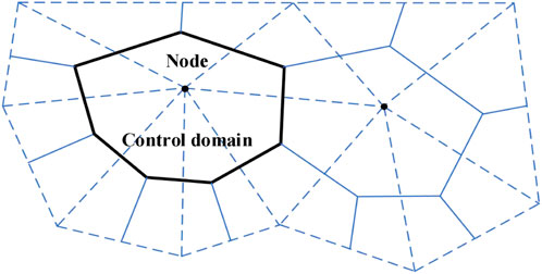
FIGURE 1. Discrete diagram of the flow plane: triangular elements (dashed lines), nodes, and computational domains (solid lines).

Therefore, the proppant thickness can be expressed as

$h=ca.(14)$

Based on the finite volume method, the integral of Eq. 4 over the computational domain A can be expressed as

${\int }_A\frac{\partial \left(ca\right)}{\partial t}dA+{\int }_A\left(ca{v}_p\right)dA=0.(15)$

Approximating the flux at the boundary of each computational domain, the discrete form of the transient term in Eq. 15 is given by the following equation:

${\int }_A\frac{\partial \left(ca\right)}{\partial t}dA=\frac{h^{new}-h^{old}}{\Delta t}A,(16)$

where $\Delta t$ is the time step. Based on Eq. 9, the diffusion term can be expressed in terms of fracturing fluid velocity and proppant settling velocity:

${\int }_A\nabla \cdot \left(ca{v}_p\right)dA={{\displaystyle \int }}_A\nabla \cdot \left(cav\right)dA+{{\displaystyle \int }}_A\nabla \cdot \left(ca{f}^{*}\left(c\right)v_{stokes}\right)dA.(17)$

Based on the Gaussian divergence theorem, an integral over a computational domain can be converted to an integral over a polygon boundary as follows:

${\int }_A\nabla \cdot \left(ca{v}_p\right)dA={{\displaystyle \int }}_{\wp }cav\cdot \mathrm{n}dA+{{\displaystyle \int }}_{\wp }ca{f}^{*}\left(c\right)v_{stokes}\cdot \mathrm{n}dA,(18)$

where $\mathrm{n}$ is the outer normal vector of the boundary of the computational domain. Let q = a·v; then, the diffusion term of the carrier fluid in Eq. 18 can be expressed as

${\int }_{\wp }cav\cdot \mathrm{n}dA={\int }_{\wp }c\mathrm{q}\cdot \mathrm{n}dA.(19)$

The discrete form of the proppant diffusion term is given by the following equation:

${\int }_{\wp }c\mathrm{q}\cdot \mathrm{n}dA={\displaystyle \sum _s}{c}_s{\left(\mathrm{q}\cdot \mathrm{n}\right)}_s{L}_s,(20)$

where ${\sum }_S$ represents the sum of the flux at each boundary of the computational domain and $L_s$ is the length of each boundary. Vector $\mathrm{n}$ is shown in Figure 2. The choice of the value of $c_s$ depends on the numerical solution method used. In this study, the upwind scheme is used to solve the problem, and the upwind scheme is unconditionally stable. Therefore, the value of parameter $c_s$ is obtained from upstream of the flow:

$c_s=\left\{\begin{array}{ccc}{c}_{P_1}& if& \mathrm{q}\cdot \mathrm{n}>0\\ c_{P_2}& if& \mathrm{q}\cdot \mathrm{n}<0\end{array}\right..(21)$

FIGURE 2

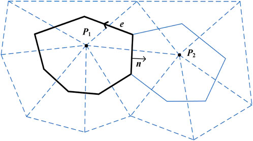
FIGURE 2. Computational domain of the upwind scheme.

The settlement–diffusion term of the proppant in Eq. 18 is a non-linear function of the principal variable c, and its numerical discrete form is as follows:

${\int }_{\wp }ca{f}^{*}\left(c\right)v_{stokes}\cdot \mathrm{n}dA={\displaystyle \sum _s}{h}_s{\left(f^{*}\left(c\right)v_{stokes}\cdot \mathrm{n}\right)}_s{L}_s,(22)$

where $h=ca$, $\overline{c}$ is the average value of $c$ at the three nodes of the triangular element, and:

$h_s=\left\{\begin{array}{ccc}{h}_{P_1}& if& v_{stokes}\cdot \mathrm{n}>0\\ h_{P_2}& if& v_{stokes}\cdot \mathrm{n}<0\end{array}\right..(23)$

By combining Eqs 14, 15, 19, and 21, the discretization equations within each computational domain can be expressed as

$h^{new}=h^{old}+\frac{\Delta t}{A}\left[{\displaystyle \sum _s}{c}_s{\left(\mathrm{q}\cdot \mathrm{n}\right)}_s{L}_s-{\displaystyle \sum _s}{h}_s{\left(f^{*}\left(c\right)v_{stokes}\cdot \mathrm{n}\right)}_s{L}_s\right].(24)$

In the explicit numerical solution process, the values of the variables on the right side of Eq. 24 are all from the previous time step. After obtaining the proppant thickness at the new time step, the proppant volume fraction was updated using Eq. 13. In this model, proppant plugging in the fracture was considered. When a blockage occurs, the proppant stops flowing, but the fluid can still pass through by setting a fixed permeability value for the blocked proppant. When the permeability is set to 0, it means that fluid cannot pass through the blocked area. In the case of the intersection of two fractures, the computational domains of the nodes at the intersection of fractures are on the two fracture surfaces, as shown in Figure 3:

FIGURE 3

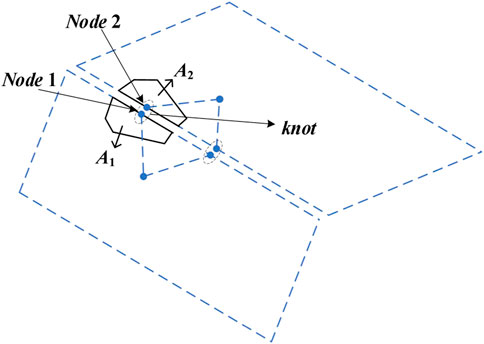
FIGURE 3. Two intersecting flow planes with triangular elements, edge nodes, and computational domains (dark colors).

Each flow plane is discretized into triangular elements. Nodes 1 and 2 located at plane intersections are grouped as “knot.” The compute domains of nodes 1 and 2 are pooled together, and the results are assigned to the knot:

$A_{knot}=A_1+A_2.(25)$

In addition, the fracture width of the knot is obtained by weighted average, given as follows:

$a_{knot}=\frac{a_1{A}_1+a_2{A}_2}{A_{knot}}.(26)$

The new proppant thickness $h_{knot}$ at the boundary node can be calculated using Eq. 24. The new proppant concentration $c_{knot}$ can be expressed as $c_{knot}=h_{knot}/a_{knot}$. The new thickness of the proppant at nodes 1 and 2 is $h_1=c_{knot}{a}_1$ and $h_2=c_{knot}{a}_2$, respectively. The proppant-volume balance equation at the intersection of fractures is

$h_{knot}{A}_{knot}=a_1{A}_1+a_2{A}_2.(27)$

The stability time step of proppant transport is calculated by considering the Courant–Friedrichs–Lewy (CFL) condition. In this case, the Courant number is defined as

$c_{\mathrm{c}}=\frac{v\Delta t}{\Delta x},(28)$

where $\Delta t$ is the time step and $\Delta x$ is the size of the discrete elements. Moreover, the conditions of stability are

$0\le v\le 1.(29)$

Therefore, based on Eq. 28, the stability time step equation can be expressed as

$\Delta t=\alpha \frac{\Delta L_{\min }}{\left|v_{p,\max }\right|},(30)$

where $\Delta L_{\min }$ is the smallest element size; $\alpha$ is the angle between the two fracture surfaces; and $\left|v_{p,\max }\right|$ is the maximum proppant velocity in the fractures.

2.3 Model comparison and validation

The solution of the model in this paper is based on ITASCA software (ITASCACG, 2024). The simulation results provided by Shiozawa and McClure (2016) and Chang (2017b) are shown in Figures 4A, B, respectively, which can be used to compare and validate the model in this study. Under the same input parameters, the results of the model established in this paper are shown in Figure 4C, which are consistent with the results in the published reference. The longitudinal variation in the fracture width in this model is ignored; therefore, the proppant can reach the bottom of the fracture. Compared to the height of proppant blockage, the results of the model established in this study are very close to the published reference.

FIGURE 4

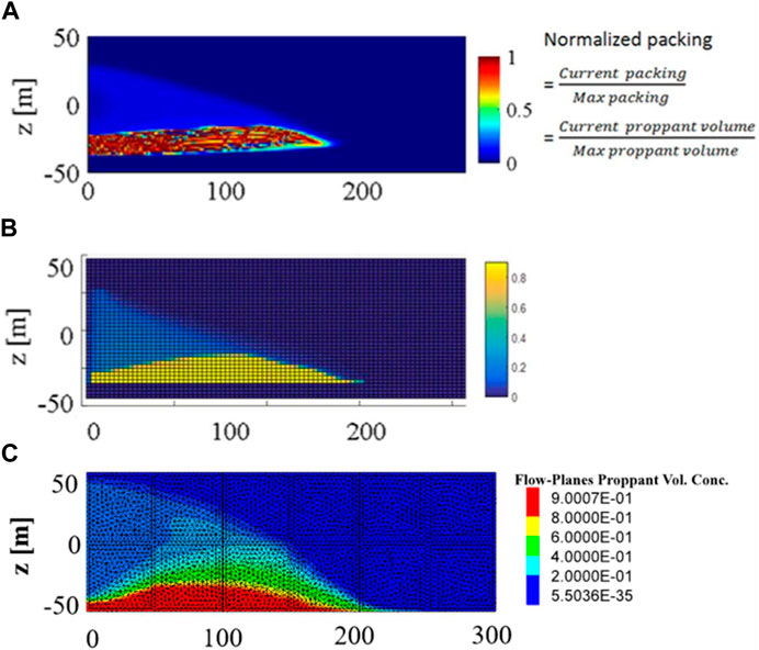
FIGURE 4. Model comparison and verification.

3 Results and discussion

3.1 Proppant transport within a single fracture

In this section, different proppant pumping strategies for a single fracture are studied, such as fixed-proppant concentration injection, stepwise increasing proppant concentration injection, and proppant slug injection. The main input parameters and values of the numerical simulation are shown in Table 1.

TABLE 1

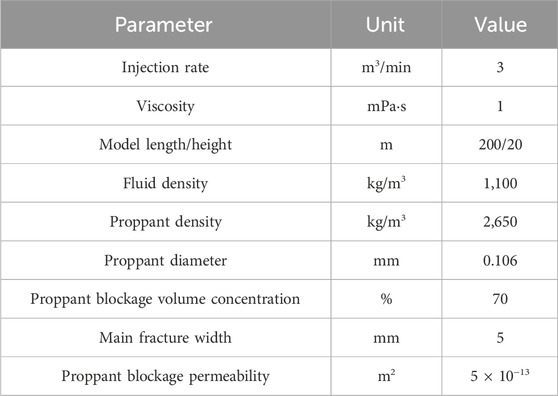
TABLE 1. Model input parameters.

3.1.1 Injection of the proppant with a constant concentration

In this section, the effect of proppant injection concentration (PIC) on its transport is studied when the PIC is constant. The PICs were set to 0.06, 0.08, and 0.10 (the concentrations in this study are all volumetric ratios). In all the cases in this paper, the total injection time simulated was 40 min. The fracturing fluid and proppant injection process is shown in Figure 5. Other input parameters are shown in Table 1, and the simulation results are shown in Figures 6, 7.

FIGURE 5

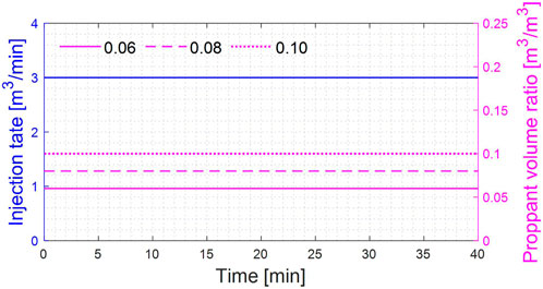
FIGURE 5. Fracturing fluid and proppant injection process.

FIGURE 6

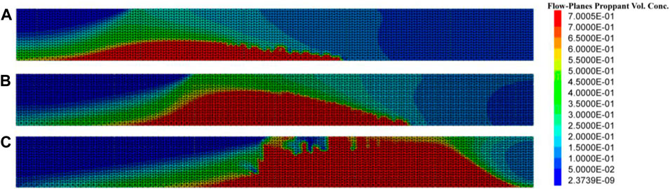
FIGURE 6. Proppant distribution at the moment of stopping injection; (A) proppant injection concentration (PIC) = 0.06; (B) PIC = 0.08; and (C) PIC = 0.10.

FIGURE 7

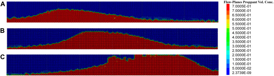
FIGURE 7. Proppant distribution at the moment of complete proppant settlement; (A) PIC = 0.06; (B) PIC = 0.08; and (C) PIC = 0.10.

Figures 6, 7 show the proppant distribution at the moment of stopping injection and proppant complete settlement, respectively. It can be observed that when the PIC is 0.06, the maximum dune height during the injection process is 8 m, and the maximum dune height after complete settlement is 13 m. When the PIC is 0.08, the maximum dune height during the injection process is 14 m, and the maximum dune height after complete settlement is 17 m. Comparing the two cases where the PIC is 0.06 and 0.08, the PIC increased by 33%, the maximum dune height during the injection process increased by 75%, the maximum dune height increased by 30.8% after complete proppant settlement, and the distance from the dune to the bottomhole significantly decreased. When the PIC increased to 0.10, the distance from the dune to the bottomhole decreased sharply, and proppant blockage occurred.

3.1.2 Injection of the proppant with a stepwise increasing concentration

The injection strategy of a stepwise increasing proppant concentration is also commonly used in hydraulic fracturing. In this section, stepwise increasing proppant concentration strategies for proppant transport are studied with three different average proppant injection concentrations. The average PICs were 0.09, 0.10, and 0.11. If the fracturing process is divided into N stages and the average PIC is M, the PIC in the first stage is 2*M/(N+1), and the concentration needs to be increased by 2*M/(N+1) in each subsequent stage. In this section of the study, the fracturing process was divided into eight stages, and the fracturing fluid and proppant injection process is shown in Figure 8. The simulation results are shown in Figures 9, 10.

FIGURE 8

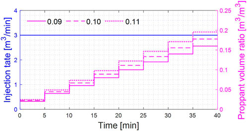
FIGURE 8. Fracturing fluid and proppant injection process.

FIGURE 9

FIGURE 9. Proppant distribution at the moment of stopping injection; (A) average PIC = 0.09; (B) average PIC = 0.10; and (C) average PIC = 0.11.

FIGURE 10

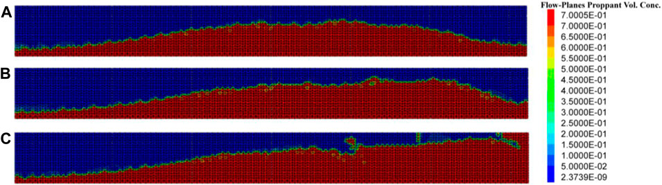
FIGURE 10. Proppant distribution at the moment of proppant complete settlement; (A) average PIC = 0.09; (B) average PIC = 0.10; and (C) average PIC = 0.11.

Figures 9, 10 show that when the average PIC is 0.09, the maximum dune height during the injection process is 7 m, and the maximum dune height after complete settlement is 14 m. When the average PIC is 0.10, the maximum dune height during the injection process is 9 m, and the maximum dune height after complete settlement is 16 m. Comparing the two cases where the average PIC is 0.09 and 0.10, the PIC increased by 11%, the maximum dune height during the injection process increased by 28.6%, and the maximum dune height increased by 14.3% after complete proppant settlement. Compared with the strategy where concentration is constant, the strategy of a stepwise increasing concentration can make the proppant distribution in the fracture more uniform. Moreover, when using the strategy of a stepwise increasing concentration, proppant blockage only occurs when the average PIC is greater than 0.11. This means that the strategy of a stepwise increasing concentration can increase the injection volume of the proppant by 25%. Furthermore, the distance from the dune to the bottomhole will also be significantly reduced.

3.1.3 Periodic injection of the proppant with a constant concentration

The periodic injection of the proppant is also a commonly used strategy in hydraulic fracturing. Periodic injection of the proppant is achieved through alternating injections of the proppant-carrying fluid and isolation fluid. To ensure a constant total injection volume, it is necessary to increase the concentration of the proppant-carrying fluid while increasing the injection volume of the isolation fluid. In this section, 8 stages of sand-carrying fluid and eight stages of isolation fluid were set in the simulation cases, and the total time for injecting one stage of the proppant-carrying fluid and one stage of isolation fluid was 5 min. When the average PIC is M, and the injection time for one stage of the proppant-carrying fluid and isolation fluid is t₁ and t₂, respectively, the PIC for each stage of the proppant-carrying fluid is M*(t₁+t₂)/t₁. In this section, m = 0.08. The fracturing fluid and proppant injection process is shown in Figure 11, and the simulation results are shown in Figures 12, 13.

FIGURE 11

FIGURE 11. Fracturing fluid and proppant injection process.

FIGURE 12

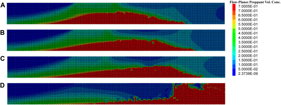
FIGURE 12. Proppant distribution at the moment of stopping injection; (A) injection time of isolation fluid (ITIF) = 0.5 min (B) ITIF = 1 min; (C) ITIF = 1.5 min; and (D) ITIF = 2 min.

FIGURE 13

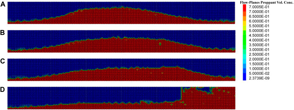
FIGURE 13. Proppant distribution at the moment of proppant complete settlement; (A) ITIF = 0.5 min; (B) ITIF = 1 min; (C) ITIF = 1.5 min; and (D) ITIF = 2 min.

The simulation results show that when the injection time of the proppant-carrying fluid and isolation fluid is 4.5 min and 0.5 min, respectively, the maximum dune height during the injection process is 12 m, and the maximum dune height after complete settlement is 15 m. When the injection time of the proppant-carrying fluid and isolation fluid is 4 and 1 min, respectively, the maximum dune height during the injection process is 11 m, and the maximum dune height after complete settlement is 13 m. By comparison, it can be seen that increasing the injection volume of the isolation fluid can reduce the dune height and also make the distribution of the proppant more uniform and reduce the distance from the dune to the bottomhole. However, since the concentration of the proppant-carrying fluid also increases with the increase in the injection volume of the isolation fluid, proppant blockage will occur when the injection time of each stage of the isolation fluid is increased to 2 min.

3.1.4 Periodic injection of the proppant with a stepwise increasing concentration

The periodic injection of the proppant with a stepwise increasing concentration is studied in this section. If the fracturing process is divided into N stages, the average PIC is M, and the injection time for one stage of proppant-carrying fluid and isolation fluid is t₁ and t₂ respectively, the PIC in the first stage is 2M*(t₁+t₂)/t₁/(N+1), and the concentration needs to be increased by 2M*(t₁+t₂)/t₁/(N+1) in each subsequent stage. In this section, 8 stages of sand-carrying fluid and 8 stages of isolation fluid were set in the simulation cases (here, M = 8), and the total time for injecting one stage of the proppant-carrying fluid and one stage of the isolation fluid was 5 min. The fracturing fluid and proppant injection process is shown in Figures 14, 15. The simulation results are shown in Figures 16, 17.

FIGURE 14

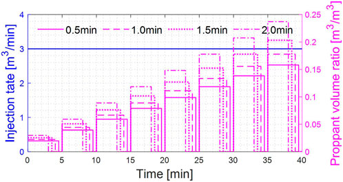
FIGURE 14. Fracturing fluid and proppant injection process.

FIGURE 15

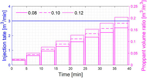
FIGURE 15. Fracturing fluid and proppant injection process.

FIGURE 16

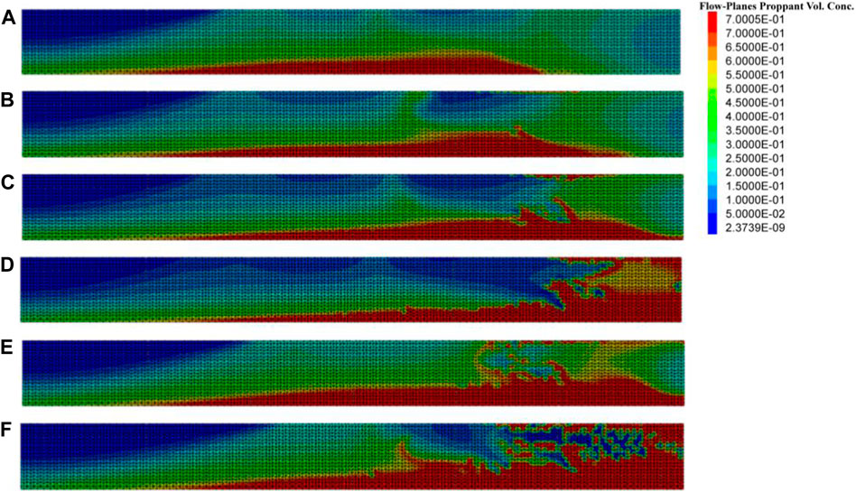
FIGURE 16. Proppant distribution at the moment of stopping injection; (A) ITIF = 0.5 min, average PIC = 0.08; (B) ITIF = 1 min, average PIC = 0.08; (C) ITIF = 1.5 min, average PIC = 0.08; (D) ITIF = 2 min, average PIC = 0.08; (E) ITIF = 0.5 min, average PIC = 0.10; and (F) ITIF = 0.5 min, average PIC = 0.12.

FIGURE 17

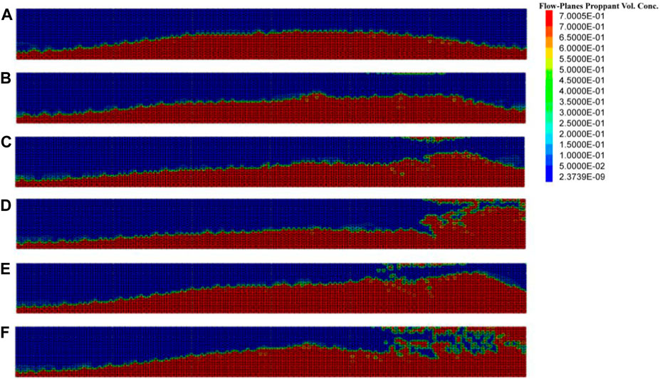
FIGURE 17. Proppant distribution at the moment of complete proppant settlement; (A) ITIF = 0.5 min, average PIC = 0.08; (B) ITIF = 1 min, average PIC = 0.08; (C) ITIF = 1.5 min, average PIC = 0.08; (D) ITIF = 2 min, average PIC = 0.08; (E) ITIF = 0.5 min, average PIC = 0.10; and (F) ITIF = 0.5 min, average PIC = 0.12.

Figures 16A–D and Figures 17A–D show the distribution of the proppant under different injection volume ratios of the proppant-carrying fluid and isolation fluid when the average PIC is 0.08, respectively. When the injection volume ratios of the proppant-carrying fluid and isolation fluid are 9:1, 8:2, and 7:3, respectively, the maximum dune height during the injection process is 5, 7, and 10 m, and the maximum dune height after complete settlement is 11, 12, and 14 m, respectively. The maximum dune height is positively correlated with the volume of the injected isolation fluid, and when the ratio is 6:4, proppant blockage will occur in hydraulic fractures. Compared to the injection strategy with a constant concentration, the proppant distribution under the periodic injection strategy with a stepwise increasing concentration is more uniform. In addition, the transport process of the proppant with average injection concentrations of 0.10 and 0.12 was studied when the volume ratio of the proppant-carrying fluid to isolation fluid was 9:1, as shown in Figures 16A, B. Compared to the injection strategy with a constant concentration, the periodic injection strategy with a stepwise increasing concentration can increase the proppant injection volume by 25% and reduce the distance from the dune to the bottomhole.

3.2 Proppant transport within multi-level branching fractures

This section investigates the transport of the proppant under multi-level fractures, and the physical model of hydraulic fractures is shown in Figure 18. The effects of the PIC, second-level fracture width, number of second-level fractures, and second-level fracture angle on proppant transport were studied. The simulation parameters are shown in Table 2, and other parameters are shown in Table 1. The numerical simulation results are shown in Figure 19.

FIGURE 18

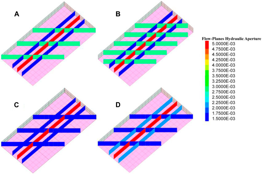
FIGURE 18. Multi-level fracture physical model:(A,B) are different numbers of branch fractures; (C,D) are different branch fracture widths.

TABLE 2

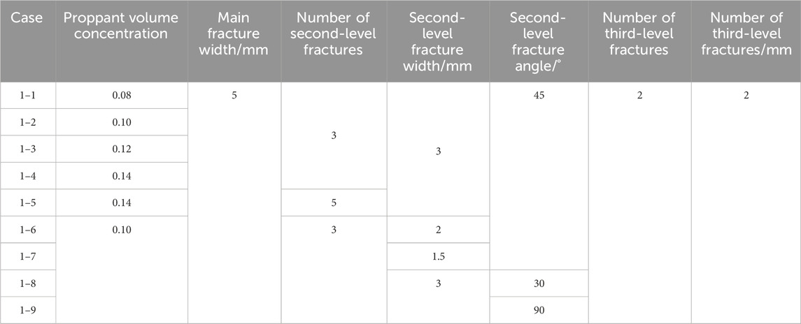
TABLE 2. Input parameters for the simulation of proppant transport within multi-level fractures.

FIGURE 19

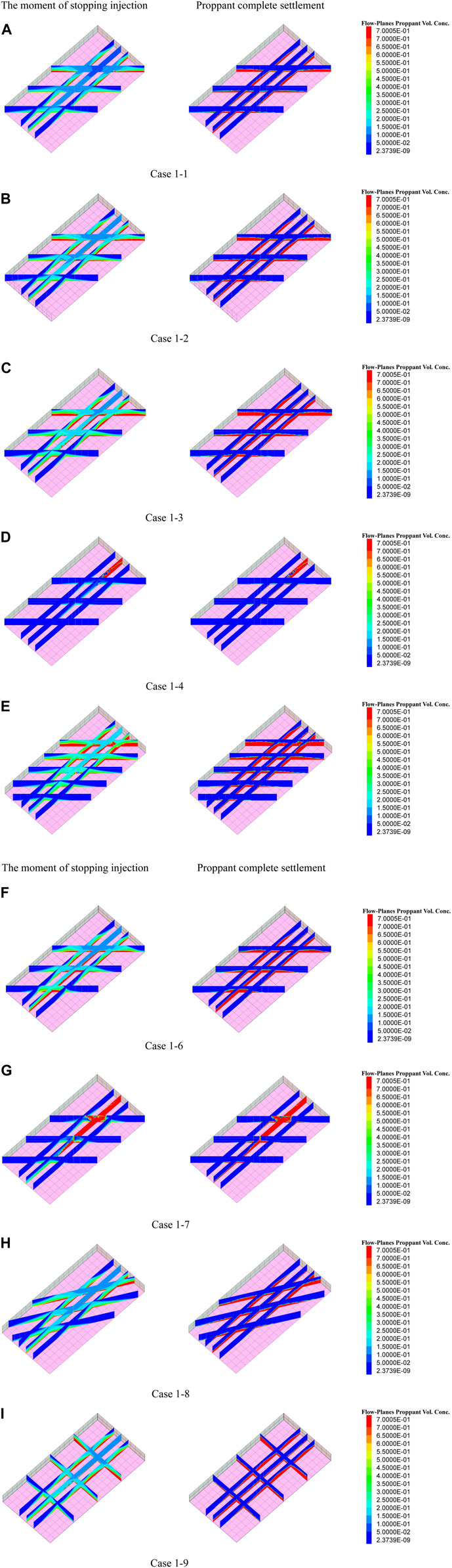
FIGURE 19. (Continued).

From cases 1–1, 1–2, 1–3, and 1–4, it can be observed that proppant blockage does not occur if the PIC is less than or equal to 0.12. Compared to the results in the previous section, the injection volume of the proppant increased by 50% in the case of multi-level hydraulic fractures. Comparing cases 1–4 and 1–5 showed that if more branch fractures are activated during the fracturing process, the risk of proppant blockage will be greatly reduced. Comparing cases 1–2, 1–6, and 1–7 showed that the dune height of the main fracture is negatively correlated with the second-level fracture width. When the width of the second-level fracture further decreases to 1.5 mm, the proppant blockage will occur first in the second-level fracture and then in the main fracture. Comparing cases 1–2, 1–8, and 1–9 showed that if the width of the second-level fracture does not change, the influence of the angle of the second-level fracture on the process of proppant transport is negligible.

4 Conclusion

In this study, a new proppant transport model was established based on the Euler method. In this model, the proppant plugging element allows fluid to pass through. Based on this model, the proppant plugging process was successfully simulated. The proppant transport and ultimate injection concentration under different injection modes were also discussed. The main conclusions are as follows:

(1) Compared with the strategy with a constant concentration, the strategy of a stepwise increasing concentration can make the proppant distribution in the fracture more uniform.

(2) The strategy of a stepwise increasing concentration can increase the injection volume of the proppant by 25%. Furthermore, the distance from the dune to the bottomhole will also be significantly reduced.

(3) Using the strategy of the periodic injection proppant, increasing the injection volume of the isolation fluid can reduce the dune height, make the distribution of the proppant more uniform, and reduce the distance from the dune to the bottomhole.

(4) Compared to the injection strategy with a constant concentration, the periodic injection strategy with a stepwise increasing concentration also can increase the proppant injection volume by 25% and reduce the distance from the dune to the bottomhole.

(5) When the number of the second-level fractures increases by 67%, proppant injection can increase by 17%. When the second-level fracture width was reduced by 50%, proppant injection was reduced by 17%. That means, if more branch fractures are activated during the fracturing process, the risk of proppant blockage will be greatly reduced. Furthermore, if the activated branch fracture width is small, the risk of proppant blockage increases dramatically.

Data availability statement

The original contributions presented in the study are included in the article/Supplementary Material; further inquiries can be directed to the corresponding authors.

Author contributions

JW: conceptualization, data curation, formal analysis, funding acquisition, investigation, methodology, project administration, resources, software, supervision, validation, visualization, writing–original draft, and writing–review and editing. YH: writing–original draft and writing–review and editing. BZ: conceptualization, data curation, formal analysis, funding acquisition, investigation, methodology, project administration, resources, software, supervision, validation, visualization, writing–original draft, and writing–review and editing. HH: writing–original draft and writing–review and editing. JG: conceptualization, data curation, formal analysis, funding acquisition, investigation, methodology, project administration, resources, software, supervision, validation, visualization, writing–original draft, and writing–review and editing. YG: conceptualization, data curation, formal analysis, funding acquisition, investigation, methodology, project administration, resources, software, supervision, validation, visualization, writing–original draft, and writing–review and editing.

Funding

The author(s) declare that financial support was received for the research, authorship, and/or publication of this article. This work was financially supported by the “Research on collaborative optimization and real-time regulation of deep shale fracturing parameters driven by big data” (52374045).

Conflict of interest

Authors JW, ZB, HH, and JG were employed by PetroChina Southwest Oil & Gas Field Company.

The remaining authors declare that the research was conducted in the absence of any commercial or financial relationships that could be construed as a potential conflict of interest.

Publisher’s note

All claims expressed in this article are solely those of the authors and do not necessarily represent those of their affiliated organizations, or those of the publisher, the editors, and the reviewers. Any product that may be evaluated in this article, or claim that may be made by its manufacturer, is not guaranteed or endorsed by the publisher.

References

Alotaibi, M. A., and Miskimins, J. L., Slickwater proppant transport in hydraulic fractures: new experimental findings and scalable correlation. SPE Prod. Operations, 2018, 33(02): 164–178. doi:10.2118/174828-pa

CrossRef Full Text | Google Scholar

Batchelor, G. K. (1967). An introduction to fluid dynamics. Cambridge, United Kingdom: Cambridge University Press.

Google Scholar

Bhandakkar, P., Siddhamshetty, P., and Kwon, J. S. I. (2020). Numerical study of the effect of propped surface area and fracture conductivity on shale gas production: application for multi-size proppant pumping schedule design. J. Nat. Gas Sci. Eng. 79, 103349. doi:10.1016/j.jngse.2020.103349

CrossRef Full Text | Google Scholar

Chang, O., Dilmore, R., and Wang, J. Y. (2017a). Model development of proppant transport through hydraulic fracture network and parametric study. J. Petroleum Sci. Eng. 150, 224–237. doi:10.1016/j.petrol.2016.12.003

CrossRef Full Text | Google Scholar

Chang, O., Dilmore, R., and Wang, J. Y. (2017b). Model development of proppant transport through hydraulic fracture network and parametric study. J. Petroleum Sci. Eng. 150, 224–237. doi:10.1016/j.petrol.2016.12.003

CrossRef Full Text | Google Scholar

Dayan, A., Stracener, S. M., and Clark, P. E. (2009). “Proppant transport in slick-water fracturing of shale-gas formations,” in SPE Annual Technical Conference and Exhibition. SPE, 2009: SPE-125068-MS, New Orleans, Louisiana, October, 2009.

CrossRef Full Text | Google Scholar

He, Y., Chen, Z., Li, X., Yang, Z., Jiang, M., and Ran, L. (2023). Self-supporting conductivity in shallow and ultra shallow shale reservoirs: under hydraulic, CO2 and Sc-CO2 fracturing. Geoenergy Sci. Eng. 223, 211557. doi:10.1016/j.geoen.2023.211557

CrossRef Full Text | Google Scholar

Hu, X., Wu, K., Li, G., Tang, J., and Shen, Z., Effect of proppant addition schedule on the proppant distribution in a straight fracture for slickwater treatment. J. Petroleum Sci. Eng., 2018, 167: 110–119. doi:10.1016/j.petrol.2018.03.081

CrossRef Full Text | Google Scholar

Huang, L., Liu, J., Zhang, F., Dontsov, E., and Damjanac, B. (2019). Exploring the influence of rock inherent heterogeneity and grain size on hydraulic fracturing using discrete element modeling. Int. J. Solids Struct. 176, 207–220. doi:10.1016/j.ijsolstr.2019.06.018

CrossRef Full Text | Google Scholar

ITASCACG (2024). 3 DEC 7.0 documentation. https://docs.itascacg.com/3dec700/3dec/docproject/source/theory/fluid/fluid_proppant.html?node2389.

Google Scholar

Kern, L. R., Perkins, T. K., and Wyant, R. E. (1959). The mechanics of sand movement in fracturing. J. Petroleum Technol. 11 (07), 55–57. doi:10.2118/1108-g

CrossRef Full Text | Google Scholar

Klingensmith, B. C., Hossaini, M., and Fleenor, S. (2015). “Considering far-field fracture connectivity in stimulation treatment designs in the Permian Basin,” in SPE/AAPG/SEG Unconventional Resources Technology Conference. URTEC, 2015: URTEC-2153821-MS, San Antonio, Texas, USA, July, 2015.

CrossRef Full Text | Google Scholar

Kou, R., Moridis, G., and Blasingame, T. (2019). “Bridging criteria and distribution correlation for proppant transport in primary and secondary fracture,” in SPE Hydraulic Fracturing Technology Conference and Exhibition, The Woodlands, Texas, USA, February, 2019.

CrossRef Full Text | Google Scholar

Li, H., Huang, B., Han, X., Wu, Z., and Zhao, X. (2023). Pulse effects on proppant transport and dune shape in vertical fracture applied in coalbed methane mining engineering during the pulse hydraulic fracturing. Geoenergy Sci. Eng. 229, 212128. doi:10.1016/j.geoen.2023.212128

CrossRef Full Text | Google Scholar

Liu, B., Yao, J., Sun, H., and Zhang, L. (2024). Revealing the effects of thermal properties of supercritical CO2 on proppant migration in supercritical CO2 fracturing. Gas Sci. Eng. 121, 205172. doi:10.1016/j.jgsce.2023.205172

CrossRef Full Text | Google Scholar

Liu, X., Zhang, X., Wen, Q., Zhang, S., Liu, Q., and Zhao, J. (2020). Experimental research on the proppant transport behavior in nonviscous and viscous fluids. Energy and Fuels 34 (12), 15969–15982. doi:10.1021/acs.energyfuels.0c02753

CrossRef Full Text | Google Scholar

Lv, M., Guo, T., Jia, X., Wen, D., Chen, M., Wang, Y., et al. (2024). Study on the pump schedule impact in hydraulic fracturing of unconventional reservoirs on proppant transport law. Energy 286, 129569. doi:10.1016/j.energy.2023.129569

CrossRef Full Text | Google Scholar

Mack, M. G., and Warpinski, N. R. (2000). Mechanics of hydraulic fracturing. Reserv. Stimul., 6–1.

Google Scholar

Patel, S., Wilson, I., Sreenivasan, H., and Krishna, S. (2024). Numerical simulations of proppant transportation in cryogenic fluids: implications on liquid helium and liquid nitrogen fracturing for subsurface hydrogen storage. Int. J. Hydrogen Energy 56, 924–936. doi:10.1016/j.ijhydene.2023.12.268

CrossRef Full Text | Google Scholar

Richardson, J. F. T. (1954). Sedimentation and fluidization: part-1. Trans. Institution Chem. Eng. 32, 35–53.

Google Scholar

Sahai, R. (2012). Laboratory evaluation of proppant transport in complex fracture systems. Golden, Colorado, United States: Colorado School of Mines.

Google Scholar

Shiozawa, S., and McClure, M. (2016). “Comparison of pseudo-3D and fully-3D simulations of proppant transport in hydraulic fractures, including gravitational settling, formation of proppant banks, tip-screen out, and fracture closure,” in SPE hydraulic fracturing technology conference, The Woodlands, Texas, USA, February, 2016.

CrossRef Full Text | Google Scholar

Sun, L., Cui, C., Wu, Z., Yang, Y., Wang, J., Trivedi, J. J., et al. (2023). An improved Eulerian scheme for calculating proppant transport in a field-scale fracture for slickwater treatment. Geoenergy Sci. Eng. 227, 211866. doi:10.1016/j.geoen.2023.211866

CrossRef Full Text | Google Scholar

Tang, H., Wen, Z., Zhang, L., Zeng, J., He, X., Wu, J., et al. (2023). A volumetric-smoothed particle hydrodynamics based Eulerian-Lagrangian framework for simulating proppant transport. J. Petroleum Sci. Eng. 220, 111129. doi:10.1016/j.petrol.2022.111129

CrossRef Full Text | Google Scholar

Tang, P., Zeng, J., Zhang, D., and Li, H. (2022). Constructing sub-scale surrogate model for proppant settling in inclined fractures from simulation data with multi-fidelity neural network. J. Petroleum Sci. Eng. 210, 110051. doi:10.1016/j.petrol.2021.110051

CrossRef Full Text | Google Scholar

Wang, X., Yao, J., Gong, L., Sun, H., Yang, Y., Zhang, L., et al. (2019). Numerical simulations of proppant deposition and transport characteristics in hydraulic fractures and fracture networks. J. Petroleum Sci. Eng. (183), 183. doi:10.1016/j.petrol.2019.106401

CrossRef Full Text | Google Scholar

Wu, C. H., and Sharma, M. M. (2016). “Effect of perforation geometry and orientation on proppant placement in perforation clusters in a horizontal well,” in SPE Hydraulic Fracturing Technology Conference, The Woodlands, Texas, USA, February, 2016.

CrossRef Full Text | Google Scholar

Xu, Y., Lei, Q., Chen, M., Wu, Q., Yang, N., Weng, D., et al. (2018). Progress and development of volume stimulation techniques. Petroleum Explor. Dev. 45 (5), 932–947. doi:10.1016/s1876-3804(18)30097-1

CrossRef Full Text | Google Scholar

Zeng, J., Li, H., and Zhang, D. (2016). Numerical simulation of proppant transport in hydraulic fracture with the upscaling CFD-DEM method. J. Nat. Gas Sci. Eng. 33, 264–277. doi:10.1016/j.jngse.2016.05.030

CrossRef Full Text | Google Scholar

Zeng, J., Li, H., and Zhang, D. (2021). Direct numerical simulation of proppant transport in hydraulic fractures with the immersed boundary method and multi-sphere modeling. Appl. Math. Model. 91, 590–613. doi:10.1016/j.apm.2020.10.005

CrossRef Full Text | Google Scholar

Zhang, B., Gamage, R. P., Zhang, C., and Ma, T. (2023). On the correlation between proppant addition strategy and distribution. Gas Sci. Eng. 117, 205060. doi:10.1016/j.jgsce.2023.205060

CrossRef Full Text | Google Scholar

Zheng, Y., Wang, H., Yang, B., Hu, Y., Shen, Z., Wen, H., et al. (2020). CFD-DEM simulation of proppant transport by supercritical CO2 in a vertical planar fracture. J. Nat. Gas Sci. Eng. 84, 103647. doi:10.1016/j.jngse.2020.103647

CrossRef Full Text | Google Scholar