Deep learning-based dynamic forecasting method and application for ultra-deep fractured reservoir production

Addressing the complex challenges in dynamic production forecasting for the deep-ultra-deep fractured carbonate reservoirs in the Tarim Basin’s Tahe Oilfield, characterized by numerous influencing factors, strong temporal variations, high non-linearity, and prediction difficulties, We proposes a prediction method based on Gated Recurrent Unit networks (GRU). Initially, the production data and influencing factors are subjected to dimensionality reduction using Pearson correlation coefficient and principal component analysis methods to obtain multi-attribute time series data. Subsequently, deep learning modeling of time series data is conducted using Gated Recurrent Unit networks. The model is then optimized using the Optuna algorithm and applied to the dynamic production forecasting of the deep-ultra-deep fractured carbonate reservoirs in the Tahe Oilfield. The results demonstrate that the Gated Recurrent Unit network model optimized by Optuna excels in the dynamic production forecasting of the Tahe fractured carbonate reservoirs. Compared with the traditional method, the mean absolute error (MAE), the root mean square error (MSE) and the mean absolute percentage error (MAPE) are reduced by 0.04, 0.1 and 1.1, respectively. This method proves to be more adaptable to the production forecasting challenges of deep fractured reservoirs, providing an effective means to enhance model performance. It holds significant practical value and importance in guiding the development of fractured reservoirs.

1 Introduction

The dynamic forecasting of carbonate rock fractured-cavity reservoirs is not only a key challenge in the field of oil exploration and development but also a crucial step in achieving sustainable development and efficient production. This study is based on this context, aiming to improve the accuracy and efficiency of reservoir dynamic behavior prediction through advanced deep learning technology. Currently, although physics-driven and data-driven methods have been widely applied in this field (McQuillan, 1985; Fletcher et al., 1995; Chang et al., 2021), they still face many challenges when dealing with specific types of reservoirs, such as carbonate rock fractured-cavity reservoirs.

Physical-driven methods are based on in-depth geological knowledge, reservoir engineering theories, and fluid dynamics principles. They simulate and predict the dynamic changes of reservoirs by constructing detailed geological and complex mathematical models. This approach emphasizes a deep understanding of underground geological structures, rock physical properties, fluid flow patterns, aiming to reveal the physical mechanisms during the oil and gas extraction process (Guo et al., 2022). This method mainly includes numerical simulation and analytical model approaches. Numerical simulation methods divide the reservoir into grids, using numerical approximation of differential equations to simulate reservoir dynamic behavior, emphasizing the intrinsic physical laws of the reservoir and exploring potential dynamic features and complex interactions (Huang et al., 2011; Kang, 2013; Kang et al., 2014). Analytical model approaches model and solve the dynamic behavior of reservoirs through mathematical means. However, physical-driven methods often face challenges such as model complexity and difficulty in obtaining parameters, especially when considering reservoir geological heterogeneity and nonlinear fluid behavior.

To overcome these challenges, data-driven methods have gradually emerged. Data-driven methods are based on a large amount of measured data, utilizing statistical, data mining, machine learning, and deep learning techniques to learn patterns and correlations from data, establishing highly adaptive predictive models. This approach can better cope with the complexity of reservoir dynamics, especially in situations with a lack of detailed geological information or the need for real-time model adjustments. Although these data-driven methods have achieved some success in the dynamic production forecasting of fractured reservoirs (Rahman, 2010; Wu et al., 2011; Meng et al., 2013; Zhang et al., 2019), there are still some challenges and limitations, such as numerous influencing factors, strong nonlinear relationships, and difficulties in real-time model adjustments.

We proposes a deep learning model based on Optuna optimization, aiming to overcome the challenges and limitations in the dynamic production forecasting of fractured reservoirs. Unlike the traditional physics-driven method, this model does not rely on complex geological and mathematical models, thus avoiding the high complexity of model construction and the difficulty of parameter acquisition. At the same time, compared with traditional data-driven methods, our deep learning model can automatically learn the patterns and associations in the data by using a large number of historical production data, so as to deal with the complexity and nonlinear characteristics of reservoir dynamic behavior more effectively. Specifically, we establish a deep learning Gated Recurrent Unit (GRU) model, which is better suited to handle time series data. Using the Pearson correlation coefficient method, we extract the most influential feature parameters for the predictive indicators, eliminating the interference of redundant features. At the same time, we use the Optuna automatic tuning algorithm to optimize the hyperparameters of the GRU model, reducing the time and cost of manual tuning. This model has powerful nonlinear modeling capabilities, adapting to new data and pattern changes in dynamic environments, achieving dynamic prediction of oilfield production indicators. Therefore, our approach has significant value in improving prediction accuracy and reducing errors.

2 Methods and principles

2.1 Pearson correlation coefficient

The Pearson correlation coefficient is used to characterize the degree of correlation in the changing trend between variables, with a range of values between [-1, 1]. When it approaches 1, it indicates a strong positive correlation; when it approaches −1, it indicates a strong negative correlation; and when it is close to 0, it signifies low correlation (Cohen et al., 2009). The formula for calculation is as follows:

$\mathit{p}\left(\mathit{x},\mathit{y}\right)=\frac{\mathit{c}\mathit{o}\mathit{v}\left(\mathit{x},\mathit{y}\right)}{\mathit{\sigma }\left(\mathit{x}\right).\mathit{\sigma }\left(\mathit{y}\right)}=\frac{\mathit{E}\left[\left(\mathit{x}-{\mathit{\mu }}_{\mathit{x}}\right)\left(\mathit{y}-{\mathit{\mu }}_{\mathit{y}}\right)\right]}{\mathit{\sigma }\left(\mathit{x}\right).\mathit{\sigma }\left(\mathit{y}\right)}$

Where, x and y represent the correlated variables, μ_xand μ_y represent the means, $\sigma \left(x\right)$ and $\sigma \left(y\right)$ represent the standard deviations of x variable and y variable respectively, and cov(x,y) is the covariance between x variables and y. The strength of the variable correlation is shown in Table 1.

TABLE 1

TABLE 1. Pearson correlation coefficient values indicate the degree of correlation of the variables.

2.2 Gated Recurrent Unit

The Gated Recurrent Unit (GRU) is a variation of the Recurrent Neural Network (RNN) introduced by Cho et al. It, like the Long Short-Term Memory (LSTM), is designed to address the issues of gradient vanishing and exploding in traditional RNNs (Chung et al., 2014). Compared to LSTM, the GRU model employs fewer gate units, reducing model complexity while achieving comparable performance to LSTM in certain scenarios (Sajjad et al., 2020).

The basic structure of GRU includes an update gate and a reset gate, which control the influence of input data and the previous time step’s state on the current time step (Figure 1). The update gate determines whether the previous time step’s state is retained and participates in the current time step’s computation, while the reset gate controls whether the previous time step’s state is ignored. The introduction of these gate mechanisms allows GRU to effectively prevent gradient vanishing or exploding when handling long sequential data. Additionally, it enables GRU to learn long-term dependencies in a few training steps, thereby improving the model’s prediction accuracy.

FIGURE 1

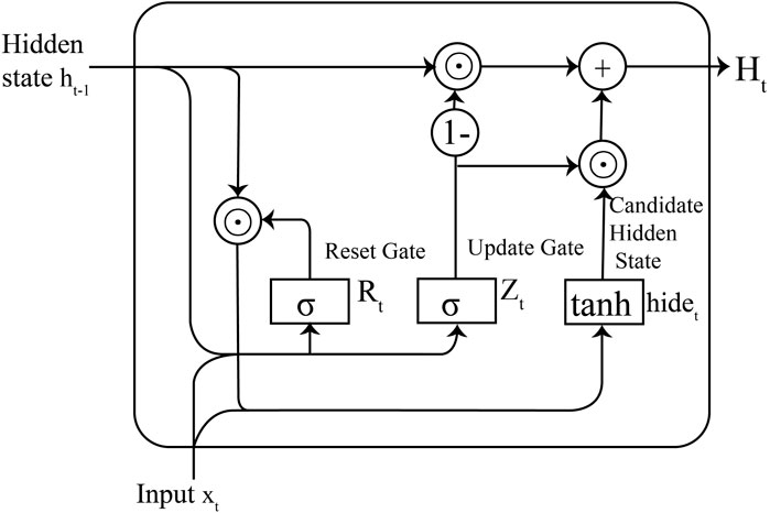
FIGURE 1. Internal structure of GRU neural network neurons.

The main computational steps are as follows:

(1) Calculate the reset gate:

$R_t=\sigma \left(W_r\cdot x_t+U_r\cdot h_{t-1}+b_r\right)$

(2) Calculate the update gate:

$Z_t=\sigma \left(W_z\cdot x_t+U_z\cdot h_{t-1}+b_z\right)$

(3) Calculate the candidate hidden state:

${hide}_t=\tanh \left(W_h\cdot x_t+R_t\odot \left(U_h\cdot h_{t-1}\right)+b_h\right)$

(4) Update the current hidden state:

$H_t=\left(1-Z_t\right)\odot h_{t-1}+Z_t\odot {hide}_t$

Where, $x_t$ is the input at time step $t$, $h_{t-1}$ is the hidden state from the previous time step, $R_t$ is the reset gate, $Z_t$ is the update gate, ${hide}_t$ is the candidate hidden state, and $H_t$ is the updated hidden state at time step t, $\sigma$ denotes the sigmoid activation function, and $\mathit{tanh}$ represents the hyperbolic tangent activation function. W_r, U_r, b_r, W_z, U_z, b_z, W_h, U_h, b_h are the weight matrices and bias parameters of the model.

2.3 Model hyperparameter tuning with the optuna framework

Hyperparameters are crucial parameters used in designing a model, including learning rate, number of iterations, layers, and the number of neurons in each layer in the context of deep learning (Khalid and Javaid, 2020). These hyperparameters directly impact the predictive accuracy of the model, and therefore, optimization is necessary to enhance model performance. Hyperparameter optimization involves combinatorial or mixed optimization, but the evaluation cost is often high, as each evaluation requires training the model with the hyperparameters to be optimized, and training deep models can take hours to days.

To address this challenge, Optuna has emerged as an automated hyperparameter optimization method. Optuna aims to minimize the value of the objective function and uses Bayesian optimization algorithms to choose the next set of hyperparameters that are likely to improve performance based on previous trial results (Ekundayo, 2020; Agrawal, 2021). Specifically, it first defines the search space for hyperparameters and selects hyperparameters in each trial according to some strategy. Then, it uses trial results to update the priority of hyperparameters so that more likely performance-improving hyperparameters are chosen in the next trial.

This automated hyperparameter optimization method brings several advantages. Firstly, it can significantly save time and resources by automating the hyperparameter optimization process, eliminating the need for manual adjustment of each parameter. Secondly, Optuna can find the optimal combination of hyperparameters, thereby improving the predictive accuracy and performance of the model.

3 Workflow

Our study establishes a workflow for predicting oilfield development indicators based on the Optuna-optimized Gated Recurrent Unit (GRU) network model. The flowchart is illustrated in Figure 2 and can be divided into the following main steps.

FIGURE 2

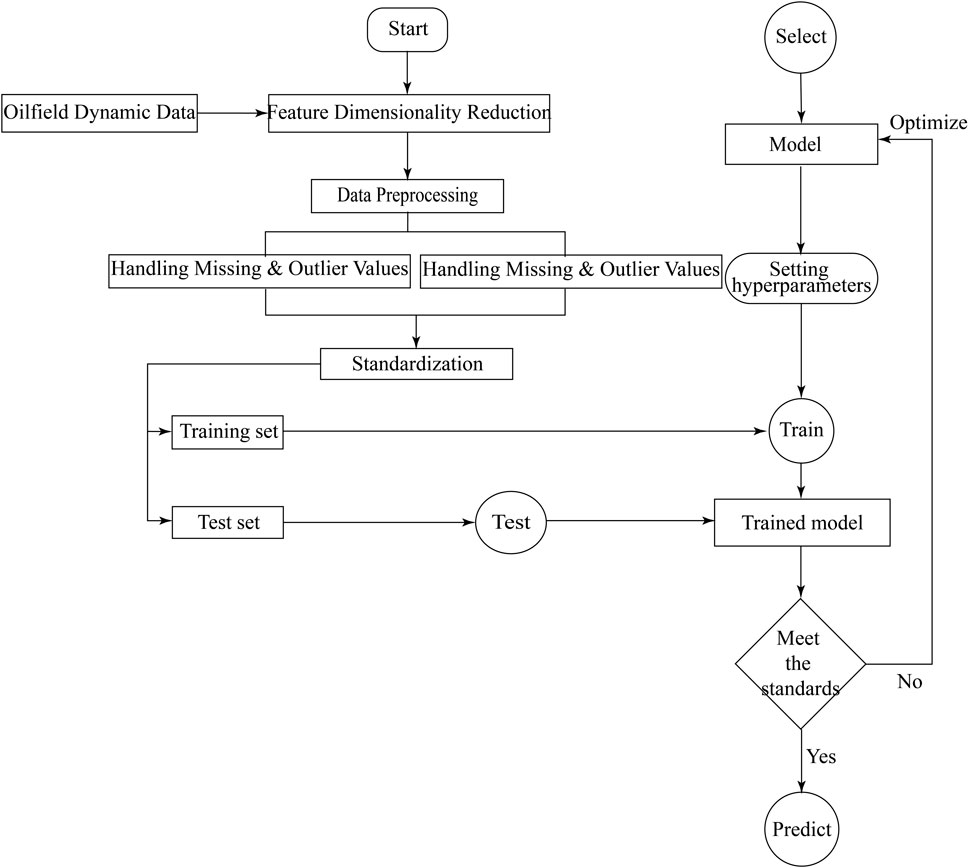
FIGURE 2. Flow chart of production index prediction based on GRU model.

3.1 Data preprocessing

This section primarily focuses on handling missing values and performing standardization on the data. When collecting data, it is common to encounter situations with a significant number of missing values. Choosing an appropriate imputation method becomes crucial. Directly removing columns with missing values may result in the loss of valuable information. Therefore, we adopted the K-nearest Neighbors (KNN) algorithm to impute missing values in the data. The KNN algorithm identifies neighboring points through distance measurement and estimates missing values by using the complete values of neighboring observations, effectively achieving data imputation (Yong et al., 2009). The specific steps are as follows: First, select the value of K as 5, and use the Euclidean distance as the measure of similarity. For each missing value, we find its 5 nearest neighbors in the feature space and compute an estimate of the missing value based on the corresponding feature values of these neighbors.

After ensuring that the data has no missing values, the next step is to standardize the data. The purpose of this step is to map the original data to a distribution with a mean of 0 and a standard deviation of 1 through linear transformation. This helps eliminate scale differences between different features, thereby improving model convergence speed and optimizing the performance and efficiency of the model. The data, after standardization, is more suitable for subsequent analysis and modeling work. The transformation function is as follows:

${x^{\prime }}_{ij}=\frac{x_{ij}-{\mu }_j}{{\sigma }_j}$

Where, ${x^{\prime }}_{ij}$ represents the value of the jth feature for the ith sample after standardization, ${\mu }_j$ denotes the mean of the jth feature, and ${\sigma }_j$ denotes the standard deviation of the jth feature.

3.2 Feature selection

There are numerous factors affecting production, and to reduce computational complexity and avoid feature redundancy, we utilized the Pearson correlation coefficient to quantitatively measure the degree of association between each feature and the target variable. Through this method, we can identify features highly correlated with the target variable, thereby avoiding the training of many irrelevant features. Additionally, principal component analysis (PCA) can be employed for feature dimensionality reduction. PCA transforms a set of highly correlated features into linearly independent feature combinations, eliminating redundant information in the data and further improving the efficiency and performance of the model (Maćkiewicz and Ratajczak, 1993; Cheng, 2014). Specifically, the covariance matrix is computed to obtain covariance information between dimensions:

$c=\frac{1}{m-1}{\left(X-\overline{X}\right)}^T\left(X-\overline{X}\right)$

Afterwards, perform an eigenvalue decomposition on the covariance matrix to identify the principal components in the data:

${Cv}_i={\lambda }_i{v}_i$

Finally, select the top k principal components to form the transformation matrix P. Multiply the original data matrix X by the transformation matrix P to obtain the reduced-dimensional matrix Y:

$P=\left[v_1,v_2,\dots ,v_k\right]$

$Y=XP$

Where, $c$ is the covariance matrix, $X$ is the original data matrix, $\overline{X}$ is the feature mean vector, $v_i$ is the feature mean vector, ${\lambda }_i$ is the matrix containing the corresponding eigenvectors.

3.3 Dataset construction

In this study, we leverage the many-to-many prediction capability of the Gated Recurrent Unit (GRU) network model to forecast future indicators based on historical production data spanning multiple months. In this approach, the value at the current time step is correlated with the values at previous time steps. By inputting data from multiple historical time steps to predict values for multiple future time steps, the model can more effectively capture this autocorrelation, thereby enhancing prediction accuracy. In contrast, predictions for a single time step may be influenced by noise and fluctuations, while the many-to-many prediction method can smooth out these fluctuations, resulting in more stable predictions.

To implement many-to-many prediction, we need to construct samples consisting of input time series and output time series.

Specifically, we set an initial time sliding window size m and an output size p, meaning we use data from m months to predict data for p months. Therefore, at time t, the model’s input data is denoted as X_t:

$\left[\begin{array}{cccc}{x}_{t,1}& x_{t,2}& \cdots & x_{t,n}\\ x_{t+1,1}& x_{t+1,2}& \cdots & x_{t+1,n}\\ x_{t+2,1}& x_{t+2,2}& \cdots & x_{t+2,n}\\ \cdots & \cdots & \cdots & \cdots \\ x_{t+m,1}& x_{t+m,2}& \cdots & x_{t+m,n}\end{array}\right]$

Where $x_{t,n}$ represents the nth feature of month t, features include yield and variables relate to yield.

The corresponding label values are Y_t are obtained as follows:

$\left[\begin{array}{c}{y}_{t+m+1}\\ y_{t+m+2}\\ \cdots \\ y_{t+m+p}\end{array}\right]$

The dataset is divided into X = {$X_1,X_2,\dots ,X_T$},Y = {$Y_1,Y_2,\dots ,Y_T$},encompassing data for a total of T months. 80% of the data is used for training the model, and the remaining 20% is used for testing the model.

3.4 Model training and hyperparameter tuning

When designing the Gated Recurrent Unit (GRU) network model, it is necessary to set some hyperparameters such as batch size, the number of layers, learning rate, and the number of training epochs. The training data is then input into the model, and a forward pass is conducted to obtain the model’s predicted output. Subsequently, the error between the predicted output and the actual values is computed. The error function is typically represented as:

$\text{MSE}=\frac{1}{N}{\displaystyle \sum _{t=1}^N}{\left(y_t-{\overline{y}}_t\right)}^2$

Where, N represents the number of future time steps, ${\widehat{y}}_t$ is the model’s predicted value at time step t, and $y_t$ is the actual production at time step.

The choice of the error function depends on the specific task; for instance, mean square error (MSE) is used for regression tasks, cross-entropy loss is employed for classification tasks, etc. Our objective is to minimize this error function to optimize the predictive performance of the model.

We utilize the Adam gradient descent algorithm for backpropagation and updating model parameters, thereby training the optimized model. Subsequently, we evaluate the model’s performance using a test dataset to assess its generalization ability. Additionally, we employ the Optuna method for hyperparameter optimization, which automatically searches for the best hyperparameter combination, further enhancing the model’s performance and efficiency. When using the Optuna method, it is necessary to specify the search range and strategy for hyperparameters, as well as define the evaluation function and target metrics. Ultimately, the optimal hyperparameter combination is obtained as the output.

3.5 Model prediction

After tuning the model hyperparameters, we obtain an optimized model that fits the current dataset well. Subsequently, we can utilize the established model to predict the production for the next N months.

4 Application example

In order to verify the reliability and scientific validity of the model, this study selects the Ordovician reservoirs in the Tarim Basin’s Tahe Oilfield as the experimental object. The reservoir depth ranges from 5000 m to 7000m, classified as a deep-ultradeep fractured reservoir. To date, the cumulative oil production from this field has exceeded 100 million tons. Utilizing over 10 years of production history dynamic data from 1,556 production wells in this reservoir, the GRU network model optimized by Optuna is employed to model and predict the monthly oil production of the oilfield. This provides a basis for future oilfield development deployment.

4.1 Establishment of monthly production model

Firstly, to ensure the quality and reliability of the data, it is necessary to address missing values and conduct standardization on the collected historical dynamic production data. Subsequently, feature selection should be applied to these data. Among the nearly 20 features collected, including monthly injection-production ratio, monthly underground loss, old well opening rate, monthly oil increase in old wells, new well opening rate, monthly oil production in new wells, natural decline rate, comprehensive decline rate, Self-Jet wells openings, pumping well openings, average dynamic liquid level, monthly oil production, monthly gas production, monthly water cut, Gas oil ratio, wellhead oil production rate, wellhead liquid production rate, production efficiency, and monthly water injection volume, some feature descriptions are shown in Table 2. We use the Pearson correlation coefficient analysis method to analyze the correlation between all features and production, as shown in Figure 3. According to the analysis results, we will exclude features with a correlation with production less than 0.2, such as new well opening rate, gas-oil ratio, and wellhead liquid production rate, which have weak correlations. Among the remaining features, we can observe correlations between them. To avoid redundancy, it is necessary to use the principal component analysis method to reduce the dimensionality of these features, transforming highly correlated features into a set of linearly independent features (Table 3). Through this series of processing and analysis, a final time series dataset with 3 independent features can be obtained, providing a comprehensive and effective data foundation for subsequent analysis and model establishment. Finally, the input data of the model are constructed as

$\left[\begin{array}{cccc}{x}_{t,1}& x_{t,2}& x_{t,3}& x_{t,o}\\ x_{t+1,1}& x_{t+1,2}& x_{t+1,3}& x_{t+1,o}\\ x_{t+2,1}& x_{t+2,2}& x_{t+2,3}& x_{t+2,o}\\ \cdots & \cdots & \cdots & \cdots \\ x_{t+m,1}& x_{t+m,2}& x_{t+m,3}& x_{t+m,o}\end{array}\right]$

Where $x_{t,1}$, $x_{t,2}$, $x_{t,3}$ represents the value of three independent features at time t after PCA dimension reduction. $x_{t,o}$ represents the oilfield production at time t.

TABLE 2

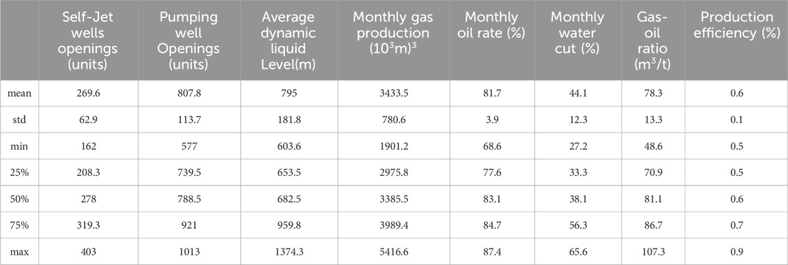
TABLE 2. The partial feature data description of the Ordovician oil reservoir in the river field of Tahe oilfield.

FIGURE 3

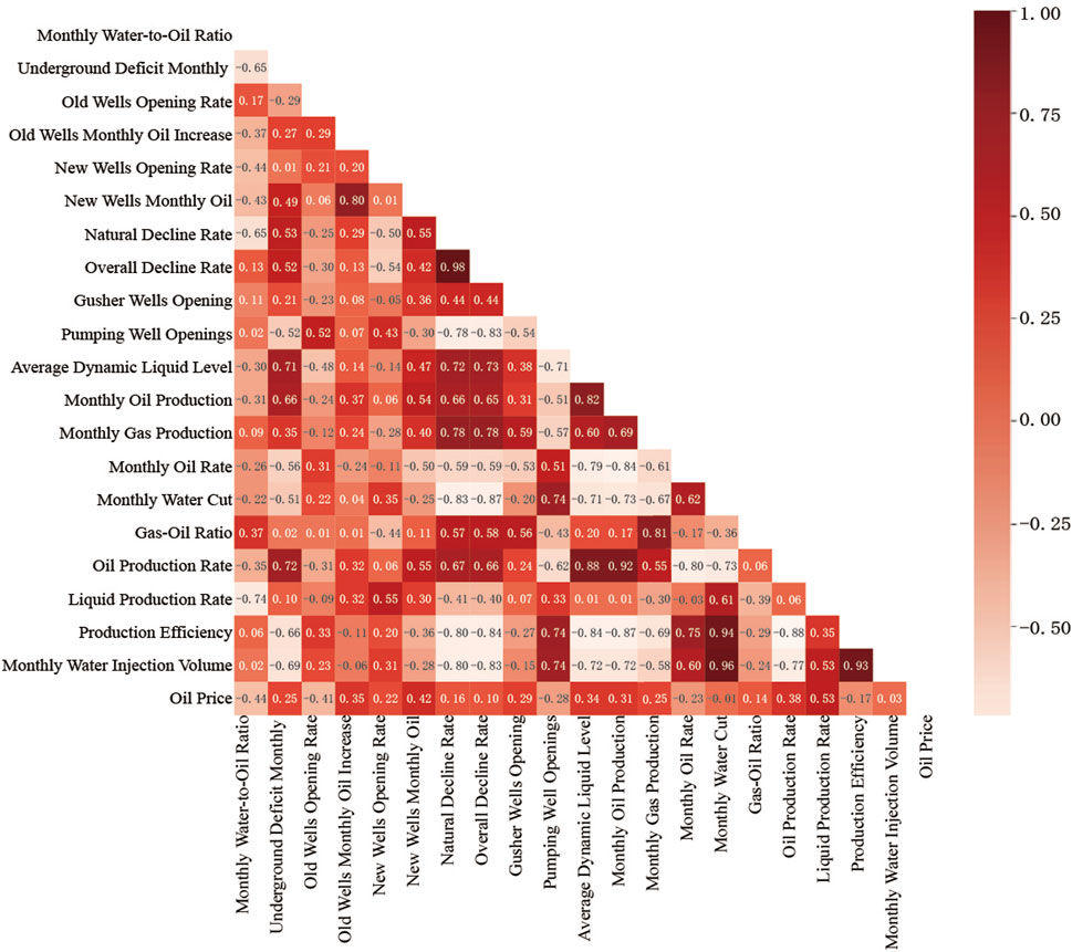
FIGURE 3. Thermodynamic diagram for correlation analysis of production characteristics based on Pearson correlation coefficient.

TABLE 3

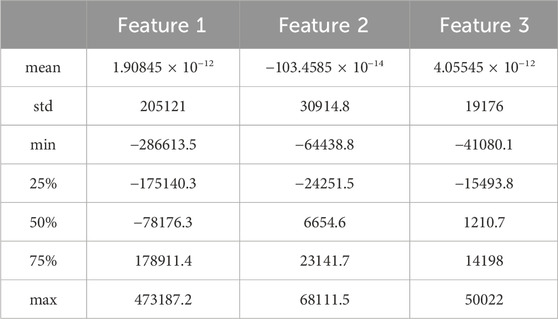
TABLE 3. Description of characteristic data after dimension reduction by principal component analysis.

the output data of the model are constructed as:

$\left[\begin{array}{c}{y}_{t+m+1}\\ y_{t+m+2}\\ \cdots \\ y_{t+m+p}\end{array}\right]$

Where $y_{t+m+p}$ represents the field production at time p in the future

In this study, the optimization of hyperparameters was considered crucial for enhancing the accuracy and efficiency of the predictive model. Therefore, we conducted an in-depth analysis of six key hyperparameters: time step size, batch size, the number of layers in the GRU network, learning rate, number of training iterations, and dropout rate. By integrating the Optuna framework, with the objective of minimizing loss on the test set, we performed a comprehensive optimization of these hyperparameters. This process not only involved searching for the optimal combination of parameters but also encompassed every stage from data processing to model training.

In the experiment predicting production indicators of fractured reservoirs, we set the hyperparameter search to 100 iterations. The results showed that varying these parameters within a certain range significantly affected the model’s predictive accuracy and efficiency. Figure 4 illustrates the ranking of the importance of hyperparameters, where the number of training rounds was the most significant factor. Figure 5 details the trend of parameter value changes during the hyperparameter search process, revealing that the model’s predictive error was minimized when the number of training rounds reached approximately 500. This indicates that the model requires a sufficient number of iterations to learn and adjust its internal weights for optimal predictive performance. The ideal range for time step size was found to be between 20 and 30, suggesting that this range allows the model to better capture the characteristics of time series data. The optimal range for the size of the hidden layer was between 200 and 300, indicating that a larger hidden layer size is necessary for the model to capture complex features in the data.

FIGURE 4

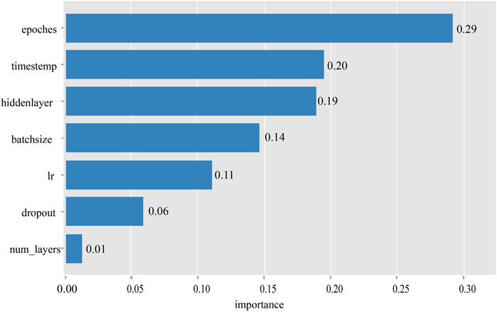
FIGURE 4. Bar chart of the importance of hyperparameters sorted by Optuna output.

FIGURE 5

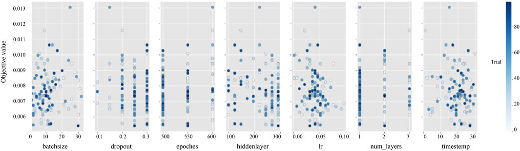
FIGURE 5. The process of hyperparameter search with changes in hyperparameter values.

Through in-depth analysis and optimization of key hyperparameters, we achieved significant improvements in model performance. We used both the optimized and unoptimized models to directly predict the total oil production of fractured reservoirs in the Tahe Oilfield. By comparing the prediction results, we found that both models had relatively low errors on the training set. However, on the test set, the optimized model showed a higher alignment with the actual monthly oil production compared to the unoptimized model, with a conformity rate of up to 89% (Figure 6). This indicates that the optimized model possesses higher predictive accuracy and stronger generalization capabilities on the test set.

FIGURE 6

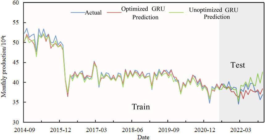
FIGURE 6. Comparison curve of actual and predicted oil production of Ordovician reservoir in the Tahe oilfield.

After comparing the GRU model used in this paper with traditional production decline methods, BP network, LSTM network, CNN network and attetion network prediction methods (see Figure 7), the results show that the prediction method based on GRU has significant advantages over other methods. To objectively evaluate the performance of various prediction methods, evaluation indicators were introduced to intuitively reflect the accuracy and generalization ability of the models (Hodson, 2022). This paper uses mean square error (MSE), mean absolute error (MAE), and mean absolute percentage error (MAPE) as key indicators of the model.

$MSE=\frac{1}{n}{\displaystyle \sum _{i=1}^n}{\left({\widehat{y}}_i-y_i\right)}^2$

$MAE=\frac{1}{n}{\displaystyle \sum _{i=1}^n}{\left({\widehat{y}}_i-y_i\right)}^2$

$MAPE=\frac{100\%}{N}{\displaystyle \sum _{i=1}^N}\left|\frac{y_i-{\widehat{y}}_i}{y_i}\right|$

FIGURE 7

FIGURE 7. Comparison of four prediction methods and actual production in the Ordovician reservoir of the Tahe oilfield.

Under these evaluation indexes, the prediction performance of GRU model was 0.06, 0.195 and 0.32, respectively, which reached the prediction standard, and the yield prediction error of GRU model was the smallest (Table 4). Although the traditional production decline method has certain advantages in simplicity and ease of use, it only considers the impact of time on production and ignores other potential factors, thus limiting the prediction accuracy. At the same time, we also compared other commonly used deep learning sequence models, including convolutional neural networks (CNN) and attention-based networks, which can fit the actual production curve well in the training set. However, when these models are applied to the test set, our GRU model shows excellent performance. The reasons behind this performance are manifold: Firstly, compared with the Long Short-Term Memory (LSTM), the GRU model has faster training speed and better memory management ability, and also overcomes the gradient vanishing problem that BP neural network often faces when dealing with long time series data. In addition, the GRU model demonstrates a more powerful ability to model time series data, effectively capturing long-term dependencies in time series. Although CNN and attention-based models perform well in tasks such as image recognition and natural language processing, they fail to show the same level of performance as GRU in the task of this study, ultra-deep fracture reservoir production prediction. This may be because the local sensing mechanism of CNN cannot adequately capture the long-term temporal dependence when dealing with sequential data with complex temporal dynamics. At the same time, although the attention model can capture long-distance dependence, it may not play its maximum performance in specific time series prediction tasks due to the complexity of the model and the limitation of training resources. These unique features make our GRU model perform exceptionally well in the task of predicting the actual production curve, providing an efficient and reliable solution for production scheduling and optimization in the oil industry. Through in-depth analysis of the performance differences between GRU and other models in this task, we further confirm the advantages of GRU in dealing with complex time series data, especially in capturing long-term dependencies, thus providing important guidance for selecting appropriate models in the future.

TABLE 4

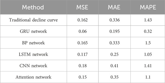
TABLE 4. MSE, MAE, MAPE values of 4 methods.

4.2 Monthly production model future forecast

Based on the production data of the past 10 years, we optimized the monthly production GRU model, especially by integrating seasonal patterns, to improve the accuracy of the forecast. As shown in Figure 8, the adjusted model is able to more accurately capture the annual seasonal trough, especially the lowest production point in February, which is highly consistent with the historical production pattern. The model forecast shows that the average monthly production of the oilfield in 2024 is 390 thousand tons, and the cumulative annual production is 4.69 million tons. In 2025, the average monthly output is 387000 tons, and the annual cumulative output is 4.62 million tons. This slow downward trend in future production is consistent with historical production trends. The forecast results with seasonal adjustment will provide a more accurate reference for Tahe Oilfield to formulate short-term production planning and deployment strategies.

FIGURE 8

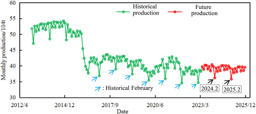
FIGURE 8. Comparison of predicted production and actual production of Ordovician reservoir in the Tahe oilfield.

5 Conclusion and recommendations

(1) After a thorough analysis of the limitations in the current methods for predicting production dynamics in fractured reservoirs, this study proposes a GRU time series model based on deep learning. Compared to traditional methods, this model demonstrates stronger capabilities in modeling time-series data, effectively addresses the vanishing gradient problem associated with BP neural networks in handling long time series data, and exhibits faster training speed and superior memory management.

(2) By employing Optuna for hyperparameter optimization, the GRU model established in this study shows higher accuracy and generalization ability in predicting production oil volume in the fractured reservoirs of the Tahe Oilfield. This allows the model to better adapt to the complex and dynamic production environment, significantly reducing prediction errors, and achieving a MSE error as low as 0.06.

(3) Our deep learning model has achieved remarkable success in dealing with short-term dynamic prediction of fractured-vuggy reservoir production. However, when the prediction time span is very long, the model performance may be limited.

Future research may focus on enhancing long-term predictive accuracy by investigating more intricate model structures, diversifying feature engineering, and refining hyperparameter tuning techniques to overcome current limitations.

Data availability statement

The datasets presented in this article are not readily available because Restricted to specific individuals, researchers, or organizations only. Requests to access the datasets should be directed to 2111210013@email.cugb.edu.cn.

Author contributions

ZD: Software, Investigation, Writing–original draft, and Writing–review & editing. DZ: Conceptualization, Methodology, Writing–original draft, Writing–review & editing, and Supervision. ZK: Resources, Conceptualization, Methodology, and Supervision. HD: Investigation, Data curation, and Writing–review & editing.

Funding

The author(s) declare that no financial support was received for the research, authorship, and/or publication of this article.

Conflict of interest

Author ZD and ZK were employed by China Petrochemical Corporation.

The remaining authors declare that the research was conducted in the absence of any commercial or financial relationships that could be construed as a potential conflict of interest.

Publisher’s note

All claims expressed in this article are solely those of the authors and do not necessarily represent those of their affiliated organizations, or those of the publisher, the editors and the reviewers. Any product that may be evaluated in this article, or claim that may be made by its manufacturer, is not guaranteed or endorsed by the publisher.

References

Agrawal, T. (2021). “Optuna and autoML.,” in Hyperparameter Optimization in Machine Learning. Berkeley, CA: Apress, 109–129. doi:10.1007/978-1-4842-6579-6_5

CrossRef Full Text | Google Scholar

Chang, B. H., Li, S. Y., Cao, W., Liu, Z. L., and Lu, L. L. (2021). Prediction methods and applications of key development indicators in fractured carbonate reservoirs. Special Oil Gas Reservoirs 28. doi:10.3969/j.issn.1006-6535.2021.02.010

CrossRef Full Text | Google Scholar

Chen, P. (2014). Research on principal component analysis and its application in feature extraction. PhD thesis. Xi’an, SN: Shaanxi Normal University

Google Scholar

Chung, J., Gulcehre, C., Cho, K., and Bengio, Y. (2014). Empirical evaluation of gated recurrent neural networks on sequence modeling. https://arxiv.org/abs/1412.3555.

Google Scholar

Cohen, I., Huang, Y., Chen, J., Benesty, J., Benesty, J., Chen, J., et al. (2009). Pearson correlation coefficient. Noise Reduct. speech Process. 1–4, 1–4. doi:10.1007/978-3-642-00296-0_5

PubMed Abstract | CrossRef Full Text | Google Scholar

Ekundayo, I. (2020). Optuna optimization based cnn-lstm model for predicting electric power consumption. PhD thesis. Dublin: National College of Ireland.

Google Scholar

Fletcher, P., Coveney, P., Hughes, T., and Methven, C. (1995). Predicting quality and performance of oil-field cements with artificial neural networks and FTIR spectroscopy. J. Petroleum Technol. 47, 129–130. doi:10.2118/28824-ms

CrossRef Full Text | Google Scholar

Guo, W., Zhang, X., Kang, L., Gao, J., and Liu, Y. (2022). Investigation of flowback behaviours in hydraulically fractured shale gas well based on physical driven method. Energies 15, 325. doi:10.3390/en15010325

CrossRef Full Text | Google Scholar

Hodson, T. O. (2022). Root-mean-square error (RMSE) or mean absolute error (MAE): when to use them or not. Geosci. Model Dev. 15, 5481–5487. doi:10.5194/gmd-15-5481-2022

CrossRef Full Text | Google Scholar

Huang, Z., Yao, J., Li, Y., Wang, C., and Lv, X. (2011). Numerical calculation of equivalent permeability tensor for fractured vuggy porous media based on homogenization theory. Commun. Comput. Phys. 9, 180–204. doi:10.4208/cicp.150709.130410a

CrossRef Full Text | Google Scholar

Kang, Z. J. (2013). Numerical simulation methods for fractured complex medium reservoirs. Daqing Petroleum Geol. Dev. 32, 55–59. doi:10.3969/j.issn.1000-3754.2013.02.009

CrossRef Full Text | Google Scholar

Kang, Z. J., Zhao, Y. Y., Zhang, Y., Lü, T., Zhang, D. L., and Cui, S. Y. (2014). Numerical simulation techniques and applications for fractured carbonate reservoirs. Petroleum Nat. Gas Geol. 35, 944–949. doi:10.11743/ogg20140621

CrossRef Full Text | Google Scholar

Khalid, R., and Javaid, N. (2020). A survey on hyperparameters optimization algorithms of forecasting models in smart grid. Sustain. Cities Soc. 61, 102275. doi:10.1016/j.scs.2020.102275

CrossRef Full Text | Google Scholar

McQuillan, H. (1985). Fracture-controlled production from the oligo-miocene asmari formation in gachsaran and bibi hakimeh fields, Carbonate petroleum reservoirs. Springer, Berlin, Germany

Google Scholar

Men, C. Q., Zhang, Q., and He, S. L., (2013). Dynamic prediction model of horizontal wells for fractured carbonate gas reservoirs. Technol. Eng. 13. doi:10.3969/j.issn.1671-1815.2013.17.004

CrossRef Full Text | Google Scholar

Rahman, M. (2010). An algorithm to model acid fracturing in carbonates: insightful sensitivity analysis. Petroleum Sci. Technol. 28, 1046–1058. doi:10.1080/10916460902967734

CrossRef Full Text | Google Scholar

Sajjad, M., Khan, Z. A., Ullah, A., Hussain, T., Ullah, W., Lee, M. Y., et al. (2020). A novel CNN-GRU-based hybrid approach for short-term residential load forecasting. Ieee Access 8, 143759–143768. doi:10.1109/access.2020.3009537

CrossRef Full Text | Google Scholar

Wu, Y. S., Di, Y., Kang, Z., and Fakcharoenphol, P. (2011). A multiple-continuum model for simulating single-phase and multiphase flow in naturally fractured vuggy reservoirs. J. Petroleum Sci. Eng. 78, 13–22. doi:10.1016/j.petrol.2011.05.004

CrossRef Full Text | Google Scholar

Yong, Z., Youwen, L., and Shixiong, X. (2009). An improved KNN text classification algorithm based on clustering. J. Comput. 4, 230–237. doi:10.4304/jcp.4.3.230-237

CrossRef Full Text | Google Scholar

Zhang, D. M., Lin, Z. H., Kang, Z. J., Wang, J. X., and Xing, L. T. (2019). Prediction of dynamic development indicators of fractured reservoirs based on EEMD-Gaussian process autoregressive model. Geol. Sci. Technol. Inf. 38, 256–263. doi:10.19509/j.cnki.dzkq.2019.0328

CrossRef Full Text | Google Scholar