Control and physical verification of 6-DOF manipulator for power inspection robots based on expert PID algorithm

To enhance the performance of power inspection robots in intricate nuclear power stations, it is necessary to improve their response speed and accuracy. This paper uses the manipulator of the power inspection robot as the primary research object, and unlike previous control algorithm research, which only remained in the software simulation stage, we constructed a set of physical verification platforms based on CAN communication and physically verified the robotic arm’s control algorithm. First, the forward motion model is established based on the geometric structure of the manipulator and D-H parameter method, and the kinematic equation of the manipulator is solved by combining geometric method and algebraic method. Secondly, in order to conduct comparison tests, we designed PID controllers and expert PID controllers by utilising the expertise of experts. The results show that compared with the traditional PID algorithm, the expert PID algorithm has a faster response speed in the control process of the manipulator. It converges quickly in 0.75 s and has a smaller overshoot, with a maximum of only 6.9%. This confirms the expert PID algorithm’s good control effect on the robotic arm, allowing the six-degree-of-freedom robotic arm to travel more accurately and swiftly along the trajectory of the target point.

1 Introduction

The application of power inspection robots (Iqbal et al., 2012; Lu et al., 2017; Menendez et al., 2017; Alhassan et al., 2020; Zhang and Dai, 2021; Zhonglin et al., 2021) is increasingly crucial for examining and upkeeping extensive and intricate power systems. The key rationale of robotics application has always been to avoid human exposure to hazardous environments and tasks ranging from scrutiny and general maintenance to decontamination and post accidental activities. To execute these activities, robots need to incorporate artificial intelligence, improved sensors capability, enhanced data fusion and compliant human like leg and hand structures for efficient motions. The commonly used PID algorithm (Borase et al., 2021) is easy to understand and implement, can quickly respond to changes in control signals, is very suitable for applications requiring stability, and can be adjusted according to different control requirements, and has a wide range of applications. However, in some complex nonlinear systems, the control accuracy of PID algorithm may not be high enough, and parameters need to be adjusted according to specific control objects and environmental conditions. Therefore, in the past studies (Parra-Vega et al., 2003; Qin et al., 2014; Krishna and Vasu, 2018; Srivastava et al., 2018), more and more scholars will fit into the traditional intelligent control algorithm of PID algorithm, through a combination between the two ways to improve control performance and precision of the algorithm. For example, Djaneye-Boundjou et al. (2016) developed a stable adaptive particle swarm optimizer to automatically adjust the parameters of PID gain; Shamseldin and Mohamed A (Shamseldin, 2021) improved the optimization model by simulating how covid-19 spreads and infuses, and proposed an efficient covid-19 optimization algorithm to obtain the optimal value of the PD/PID cascade controller. Xiao et al. (2023) also used RBF neural network to improve the tracking performance of the manipulator by updating PID parameters through errors between network output and system output.

Because the manipulator is a typical multi-input and multi-output complex system, it has the characteristics of strong coupling and nonlinear, and the special driving mode makes it difficult to establish an accurate system model in practice. For this kind of nonlinear physical system, Sliding Mode Control (SMC) has the advantages of being insensitive to system parameter changes and external interference, and has good control effect on uncertain nonlinear systems, so it is widely used in the design of manipulator control system (Peng et al., 2019; Zhang and Yan, 2019; Dai et al., 2022). However, in practical applications, the traditional sliding mode control has the problem of buffeting, that is, the motion trajectory shuttles high-frequency on both sides of the synovial surface (Wang et al., 2009). Therefore, in order to suppress the problem of cutting-edge vibration, Long et al. (2021) proposed to overlay the Actor-Critic based reinforcement learning controller with the improved sliding mode controller to improve the positioning accuracy of the flexible manipulator. Yu (2020) proposed a TSMC based on expected trajectory to asymptotically track terminal trajectory and stimulate periodic flexible vibration.

Although many intelligent control algorithms show excellent control performance and accuracy in the simulation of manipulator software, there are still many limitations. First, differences between the virtual simulation and the actual operation can lead to inaccuracies in the algorithm, which can affect the behavior of the robotic arm. Secondly, due to the simplification of the simulation environment and the lack of interference and noise in the real environment, the results of software simulation may be biased from the actual situation. Finally, software simulation requires the support of high-performance computers and complex software, which may bring high costs and technical barriers.

In this paper, a 6-DOF manipulator is used as a hardware platform to verify the control algorithm of the manipulator. Based on CAN communication, the 6-DOF manipulator realizes the control of six joint motor of the manipulator body by upper computer software. This study constructs the forward kinematics modeling of the six degrees of freedom mechanical arm and deduces a solution to the manipulator’s inverse kinematics problem, which is necessary to achieve the PC software control of the manipulator completely, and its written as M file to import into the MATLAB software. Finally, the conventional PID algorithm and expert PID algorithm were implemented in the robotic arm control system, and physical comparison experiments between intelligent control algorithms were conducted.

The paper is organized as follows. Section 2 focuses on the hardware platform used for the subsequent experiments. Section 3 is divided into three parts. The first two parts deal with the establishment of the positive motion model and the derivation of the kinematic equations, both of which are proven to be correct. The last part focuses on the design of the controller within the robotic arm control system. Section 4 presents the physical verification. The final conclusions will be provided at the end.

2 Hardware platform

2.1 Arm body

Mobile robots with manipulator (as shown in Figure 1) are currently widely utilised in real-world applications such as metropolitan highways, agriculture, mining, and power plants because they are highly adaptable, capable of completing complex tasks, and can withstand a variety of harsh indoor and outdoor conditions.

Figure 1

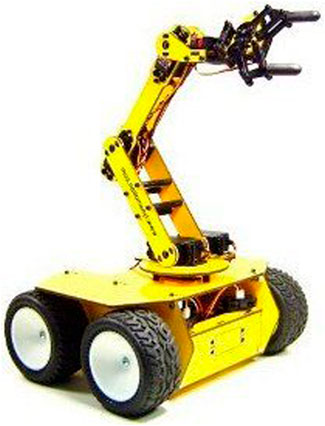
Figure 1. The actual picture of mobile robot equipped with manipulator.

In this study, we focus on the robotic arm as the research object, and as a result, we construct a physical verification platform (as shown in Figure 2) for the robotic arm control algorithms. Figure 3 shows the manipulator hardware used in this paper, which is used to validate the control effect of the intelligent control algorithm on the robotic arm entity, and the robotic arm physical object is modeled in 3D to simplify the complex geometrical structure of the robotic arm.

Figure 2

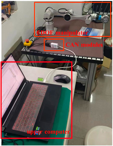
Figure 2. The actual picture of robotic arm experiment platform.

Figure 3

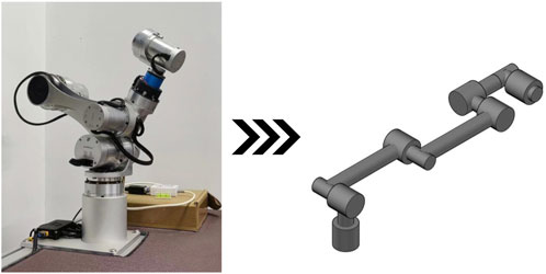
Figure 3. Simplified model of the robotic arm.

2.2 Communication protocol

Because the upper computer’s control of the 6-DOF manipulator body is actually the control of the six joint motors, it is necessary to build the communication protocol between the upper computer and the six joint motors. In the 6-DOF manipulator body, CAN communication is used to complete the data exchange between the upper computer and the six joint motors.

CAN communication as a kind of high-speed serial communication protocol, CAN use twisted-pair cable to transmit signals, is widely used in the field of servo motor control. CAN communication usually requires the use of CAN controller and CAN transceiver to realize the control of one or more servo motors, which can be directly connected with the servo drive (as shown in Figure 4) to complete the communication process. At the same time, CAN communication can also realize the speed, position and torque of the motor parameters control. In addition, CAN communication can also realize motor diagnosis and fault monitoring, improve the reliability and safety of the control system.

Figure 4

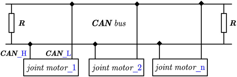
Figure 4. CAN bus structure.

The host computer that controls the manipulator CAN choose the general PC end. The control of the manipulator does not have high requirements on the system and hardware performance of the host computer. The data communication between the host computer and the manipulator body can be completed with the help of the USB to CAN module.

There are two kinds of modules that CAN complete CAN communication, one is a low-speed ordinary CAN module, and the other is a high-speed CAN module (as shown in Figure 5). The existing low-speed CAN module defines a baud rate of 115.2Kbps for data communication, and it can control the six joint motors or the whole manipulator body with the python programming environment. And after testing, when the transmission rate is 40Kbps, the bus distance can reach 1,000 m. The other high-speed closed-loop CAN communication when the communication bus length is less than or equal to 40 m, the maximum communication rate can reach 1Mbps.

Figure 5

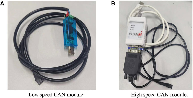
Figure 5. CAN module used in this study. (A) Low speed CAN module; (B) High speed CAN module.

In the experiment of this paper, we will also use the high-speed CAN module as the basis for data communication between the host computer and the manipulator body, define the baud rate of CAN communication as 250 Kbps, and realize the control of the six joint motors and the manipulator body with MATLAB software.

3 Robotic arm modeling and controller design

3.1 Forward kinematic analysis

According to the D-H parameter method definition (Hayat et al., 2013), a spatial geometric relationship between the connecting rods is established based on the 3D model of the robotic arm in Figure 3, and a connecting rod coordinate system is established on each robotic arm joint separately, as shown in Figure 6. The D-H parameter table of this robotic arm is then constructed based on the connecting rod coordinate system, as illustrated in Table 1.

Figure 6

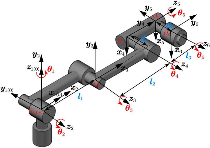
Figure 6. The link coordinate system of the whole robotic arm.

Table 1

Table 1. The D-H parameter table of the six-degree-of-freedom robotic arm.

The D-H parameters in Table 1 are brought into the positional transformation matrix (Hayat et al., 2013) in the D-H parameter method to obtain the positional transformation matrix of the robotic arm from the base coordinates {0} to the coordinate system {6} as shown in Eq. 1.

$\left\{\begin{array}{cc}{}_1{}^{0}T\left({\theta }_1\right)=\left[\begin{array}{cccc}\hfill \cos {\theta }_1\hfill & \hfill -\sin {\theta }_1\hfill & \hfill 0\hfill & \hfill 0\hfill \\ \hfill \sin {\theta }_1\hfill & \hfill \cos {\theta }_1\hfill & \hfill 0\hfill & \hfill 0\hfill \\ \hfill 0\hfill & \hfill 0\hfill & \hfill 1\hfill & \hfill 0\hfill \\ \hfill 0\hfill & \hfill 0\hfill & \hfill 0\hfill & \hfill 1\hfill \end{array}\right];\hfill & {}_2{}^{1}T\left({\theta }_2\right)=\left[\begin{array}{cccc}\hfill \cos {\theta }_2\hfill & \hfill -\sin {\theta }_2\hfill & \hfill 0\hfill & \hfill 0\hfill \\ \hfill 0\hfill & \hfill 0\hfill & \hfill -1\hfill & \hfill 0\hfill \\ \hfill \sin {\theta }_2\hfill & \hfill \cos {\theta }_2\hfill & \hfill 0\hfill & \hfill 0\hfill \\ \hfill 0\hfill & \hfill 0\hfill & \hfill 0\hfill & \hfill 1\hfill \end{array}\right];\hfill \\ {}_3{}^{2}T\left({\theta }_3\right)=\left[\begin{array}{cccc}\hfill \cos {\theta }_3\hfill & \hfill -\sin {\theta }_3\hfill & \hfill 0\hfill & \hfill l_1\hfill \\ \hfill \sin {\theta }_3\hfill & \hfill \cos {\theta }_3\hfill & \hfill 0\hfill & \hfill 0\hfill \\ \hfill 0\hfill & \hfill 0\hfill & \hfill 1\hfill & \hfill 0\hfill \\ \hfill 0\hfill & \hfill 0\hfill & \hfill 0\hfill & \hfill 1\hfill \end{array}\right];\hfill & {}_4{}^{3}T\left({\theta }_4\right)=\left[\begin{array}{cccc}\hfill \sin {\theta }_4\hfill & \hfill \cos {\theta }_4\hfill & \hfill 0\hfill & \hfill l_2\hfill \\ \hfill -\cos {\theta }_4\hfill & \hfill \sin {\theta }_4\hfill & \hfill 0\hfill & \hfill 0\hfill \\ \hfill 0\hfill & \hfill 0\hfill & \hfill 1\hfill & \hfill -d_3\hfill \\ \hfill 0\hfill & \hfill 0\hfill & \hfill 0\hfill & \hfill 1\hfill \end{array}\right];\hfill \\ {}_5{}^{4}T\left({\theta }_5\right)=\left[\begin{array}{cccc}\hfill \cos {\theta }_5\hfill & \hfill -\sin {\theta }_5\hfill & \hfill 0\hfill & \hfill 0\hfill \\ \hfill 0\hfill & \hfill 0\hfill & \hfill 1\hfill & \hfill l_3\hfill \\ \hfill -\sin {\theta }_5\hfill & \hfill -\cos {\theta }_5\hfill & \hfill 0\hfill & \hfill 0\hfill \\ \hfill 0\hfill & \hfill 0\hfill & \hfill 0\hfill & \hfill 1\hfill \end{array}\right];\hfill & {}_6{}^{5}T\left({\theta }_6\right)=\left[\begin{array}{cccc}\hfill \cos {\theta }_6\hfill & \hfill -\sin {\theta }_6\hfill & \hfill 0\hfill & \hfill 0\hfill \\ \hfill 0\hfill & \hfill 0\hfill & \hfill -1\hfill & \hfill -d_4\hfill \\ \hfill \sin {\theta }_6\hfill & \hfill \cos {\theta }_6\hfill & \hfill 0\hfill & \hfill 0\hfill \\ \hfill 0\hfill & \hfill 0\hfill & \hfill 0\hfill & \hfill 1\hfill \end{array}\right].\hfill \end{array}\right.(1)$

By continuously right-multiplying the coordinate transformation matrix in Eq. 1, the pose transformation matrix of the end effector of the robotic arm can be obtained, i.e., the pose transformation matrix of the end effector of the sixth joint relative to the base coordinate system {0}:

${}_6{}^{0}T={}_1{}^{0}T{}_2{}^{1}T{}_3{}^{2}T{}_4{}^{3}T{}_5{}^{4}T{}_6{}^{5}T=\left[\begin{array}{cccc}\hfill m_{11}\hfill & \hfill m_{12}\hfill & \hfill m_{13}\hfill & \hfill x\hfill \\ \hfill m_{21}\hfill & \hfill m_{22}\hfill & \hfill m_{23}\hfill & \hfill y\hfill \\ \hfill m_{31}\hfill & \hfill m_{32}\hfill & \hfill m_{33}\hfill & \hfill z\hfill \\ \hfill 0\hfill & \hfill 0\hfill & \hfill 0\hfill & \hfill 1\hfill \end{array}\right](2)$

where ${\left[\begin{array}{ccc}\hfill m_{11}\hfill & \hfill m_{21}\hfill & \hfill m_{31}\hfill \end{array}\right]}^T$ represents the direction of the X-axis of coordinate system {6} in the global coordinate system; ${\left[\begin{array}{ccc}\hfill m_{12}\hfill & \hfill m_{22}\hfill & \hfill m_{32}\hfill \end{array}\right]}^T$ represents the direction of the y-axis of coordinate system {6} in the global coordinate system; ${\left[\begin{array}{ccc}\hfill m_{13}\hfill & \hfill m_{23}\hfill & \hfill m_{33}\hfill \end{array}\right]}^T$ represents the direction of the Z-axis of coordinate system {6} in the global coordinate system; ${\left[\begin{array}{ccc}\hfill x\hfill & \hfill y\hfill & \hfill z\hfill \end{array}\right]}^T$ represents the position of the origin O of coordinate system {6} in the global coordinate system.

The position of the end effector of the robotic arm in the global coordinate system is:

$\left\{\begin{array}{c}x=d_4\left(\mathrm{c}{\theta }_5\mathrm{s}{\theta }_1+\mathrm{s}{\theta }_5\mathrm{c}{\theta }_{1}s{\theta }_{234}\right)-d_3\mathrm{s}{\theta }_1+l_3\mathrm{c}{\theta }_1\mathrm{c}{\theta }_{234}+l_{1}c{\theta }_{1}c{\theta }_2+l_{2}c{\theta }_{1}c{\theta }_{23}\hfill \\ y=-d_4\left(\mathrm{c}{\theta }_{5}c{\theta }_1-\mathrm{s}{\theta }_{5}s{\theta }_{1}s{\theta }_{234}\right)+d_{3}c{\theta }_1+l_{3}s{\theta }_1\mathrm{c}{\theta }_{234}+l_{1}s{\theta }_{1}c{\theta }_2+l_{2}s{\theta }_{1}c{\theta }_{23}\hfill \\ z=-d_{4}s{\theta }_5\mathrm{c}{\theta }_{234}+l_{1}s{\theta }_2+l_{2}s{\theta }_{23}+l_{3}s{\theta }_{234}\hfill \end{array}\right.(3)$

where sθ represents sin θ; cθ represents cos θ; θ₂₃ = θ₂ + θ₃; θ₂₃₄ = θ₂ + θ₃ + θ₄.

3.2 Inverse kinematics analysis

The solution of a robotic arm’s inverse kinematics is critical to the study of path planning and motion control, and many scholars have conducted extensive discussions and research in this area in recent years in order to find the optimal solution for robotic arm control among many inverse kinematics solutions (Xiao et al., 2017; Guida et al., 2019; Bodie et al., 2021; Guan et al., 2021; Dou et al., 2022). Optimization algorithms such as the particle swarm algorithm (Alkayyali and Tutunji, 2019; Zhao et al., 2022), neural network (Almusawi et al., 2016), and genetic algorithm (Gan et al., 2005) are employed to derive the optimal solutions of kinematic equations. However, adding optimization algorithms to the process of inverse kinematics solving of the robotic arm to obtain the optimal solution greatly increases the workload of the control system and significantly increases the solving time, making it unsuitable for use in practical power plants inspection and maintenance. In this study, the possibility of the presence of the inverse kinematics solution is decreased by raising the known circumstances (i.e., attitude angle) and restricting the range of joint motion, and lastly, the results of the inverse kinematics solution of the robotic arm are confined to two cases.

From the definition of the orientation angles (Meng et al., 2019), the pitch, roll and yaw angles of the end attitude of the robotic arm are defined as:

${\theta }_{234}={\theta }_{pitch\text{\_}angle};{\theta }_5={\theta }_{roll\text{\_}angle};{\theta }_6={\theta }_{yaw\text{\_}angle}(4)$

Then, we use the system of equations (Eq. 3) that includes the remaining known variables to solve the kinematic equations and obtain the numerical value of θ₁ ∼θ₄.

Multiply the first Eq. 3 by sin θ₁ and subtract the second Eq. 3 by cos θ₁, it can be obtained that:

$x\sin {\theta }_1-y\cos {\theta }_1=d_4\cos {\theta }_5-d_3(5)$

Given A = −y, B = x, C = d₄ cos θ₅ − d₃, substituting the values of A, B, C into Eq. 5, it follows that:

$A\cos {\theta }_1+B\sin {\theta }_1=C(6)$

Given $t=\tan \left(\frac{{\theta }_1}{2}\right)$, according to the double angle formula, $\cos {\theta }_1=\frac{1-t^2}{1+t^2}$, $\sin {\theta }_1=\frac{2t}{1+t^2}$. Therefore, substituting cos θ₁ and sin θ₁ into Eq. 6, it can be obtained that:

$\left(A+C\right)t^2-2Bt-\left(A-C\right)=0(7)$

Solving the above system of quadratic equations (Eq. 7), it can be obtained that:

$t=\left\{\begin{array}{cc}\frac{B\pm \sqrt{A^2+B^2-C^2}}{A+C}\hfill & A+C\ne 0\hfill \\ -\frac{A-C}{2B}\hfill & A+C=0\hfill \end{array}\right.(8)$

When A+ C = 0 and B = 0, substituting into Eq. 7 yields A = 0, so it can be known that x = y = 0, and the endpoint of the robotic arm’s end effector always lies on the Z-axis. This case will be discussed separately later. Through programming and experimental verification, it is found that for the case of in Eq. 8, the “-” sign should be taken.

Finally, from the known condition $t=\tan \left(\frac{{\theta }_1}{2}\right)$, the angle of joint one can be obtained that:

${\theta }_1=2\mathrm{a}\mathrm{r}\mathrm{c}\tan t(9)$

Given

$\begin{array}{ll}\hfill R_1& =x-d_4\left(\cos {\theta }_5\sin {\theta }_1+\sin {\theta }_5\cos {\theta }_1\sin {\theta }_{234}\right)\hfill \\ \hfill & +d_3\sin {\theta }_1-l_3\cos {\theta }_{234}\cos {\theta }_1\hfill \\ \hfill R_2& =y+d_4\left(\cos {\theta }_5\cos {\theta }_1-\sin {\theta }_5\cos {\theta }_1\sin {\theta }_{234}\right)\hfill \\ \hfill & -d_3\cos {\theta }_1-l_3\cos {\theta }_{234}\sin {\theta }_1\hfill \end{array}(10)$

By substituting R₁ from Equation 10 into the first equation of Eq. 3 and removing the variable x, and substituting R₂ from Eq. 10 into the second equation of Equation 3 and removing the variable y, the formulas for R₁ and R₂ is obtained that:

$\begin{array}{ll}\hfill R_1& =\cos {\theta }_1\left(l_1\cos {\theta }_2+l_2\cos {\theta }_{23}\right)\hfill \\ \hfill R_2& =\sin {\theta }_1\left(l_1\cos {\theta }_2+l_2\cos {\theta }_{23}\right)\hfill \end{array}(11)$

Multiplying both sides of the expression for R₁ of Eq. 11 by cos θ₁ and both sides of the expression for R₂ of Eq. 11 by sin θ₁, and then adding the two equations together, it can be obtained that:

$R_1\cos {\theta }_1+R_2\sin {\theta }_1=l_1\cos {\theta }_2+l_2\cos {\theta }_{23}(12)$

Given R₃ = R₁ cos θ₁ + R₂ sin θ₁, and substituting the expression for R₃ into Eq. 12. It can be obtained that:

$R_3=l_1\cos {\theta }_2+l_2\cos {\theta }_{23}(13)$

Given R₄ = z + d₄ sin θ₅ cos θ₂₃₄ − l₃ sin θ₂₃₄, substituting the expression for R₄ into the third equation of Eq. 3 and removing the variable z results in a new expression for R₄.

$R_4=l_1\sin {\theta }_2+l_2\sin {\theta }_{23}(14)$

Integrating Eq. 13 and Eq. 14, it can be obtained that:

$R_3\cos {\theta }_2+R_4\sin {\theta }_2=\frac{R_3^2+R_4^2+l_1^2-l_2^2}{2l_1}(15)$

Given $R_5=\frac{R_3^2+R_4^2+l_1^2-l_2^2}{2l_1}$, substituting the formula for R₅ into Eq. 15, it can be obtained that:

$R_5=R_3\cos {\theta }_2+R_4\sin {\theta }_2(16)$

Given $k=\tan \left(\frac{{\theta }_2}{2}\right)$, according to the double angle formula, $\cos {\theta }_2=\frac{1-k^2}{1+k^2}$, $\sin {\theta }_2=\frac{2k}{1+k^2}$. Therefore, substituting cos θ₂ and sin θ₂ into Eq. 16, it can be obtained that:

$\left(R_3+R_5\right)k^2-2R_{4}k-\left(R_3-R_5\right)=0(17)$

Calculating the above system of quadratic equations (Eq. 17), it can be obtained that:

$k=\left\{\begin{array}{cc}\frac{R_4\pm \sqrt{R_3^2+R_4^2-R_5^2}}{R_3+R_5}\hfill & R_3+R_5\ne 0\hfill \\ -\frac{R_3-R_5}{2R_4}\hfill & R_3+R_5=0\hfill \end{array}\right.(18)$

After experimental analysis and verification, it was found that the cases of R₃ + R₅ and R₄ = 0 do not exist. Based on the condition that the robotic arm’s end position and posture remain unchanged, there are two configurations: α configuration and β configuration (as shown in Figure 7). When the robotic arm needs to be in the α configuration, the “+” sign should be taken for the case of R₃ + R₅ ≠ 0; conversely, when the robotic arm needs to be in the β configuration, the “-” sign should be taken for the case of R₃ + R₅ ≠ 0.

Figure 7

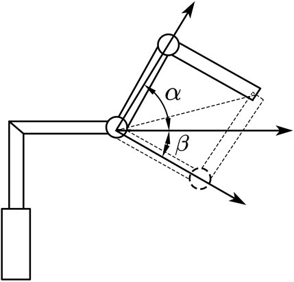
Figure 7. Two configurations of the robotic arm.

Finally, from the known condition $k=\tan \left(\frac{{\theta }_2}{2}\right)$, the angle of joint one can be obtained that:

${\theta }_2=2\mathrm{a}\mathrm{r}\mathrm{c}\tan k(19)$

Integrating Eqs 13, 14 yields the expressions for cos θ₂₃ and sin θ₂₃:

$\cos {\theta }_{23}=\frac{R_3-l_1\cos {\theta }_2}{l_2},\sin {\theta }_{23}=\frac{R_4-l_1\sin {\theta }_2}{l_2}(20)$

Given $R_6=\frac{R_3-l_1\cos {\theta }_2}{l_2},R_7=\frac{R_4-l_1\sin {\theta }_2}{l_2}$, substituting R₆ and R₇ into Eq. 20, it can be obtained that:

${\theta }_{23}=\mathrm{a}\mathrm{r}\mathrm{c}\tan \left(\frac{R_7}{R_6}\right)(21)$

Finally, the angles of joint three and joint four can be obtained that:

${\theta }_3={\theta }_{23}-{\theta }_2,{\theta }_4={\theta }_{234}-{\theta }_{23}(22)$

Combining Eqs 4, 9, 19–22, the θ₁ ∼θ₆ of the six joints of the robotic arm can be obtained:

$\left\{\begin{array}{c}{\theta }_1=2\mathrm{a}\mathrm{r}\mathrm{c}\tan t;\hfill \\ {\theta }_2=2\mathrm{a}\mathrm{r}\mathrm{c}\tan k;\hfill \\ {\theta }_3={\theta }_{23}-{\theta }_2;\hfill \\ {\theta }_4={\theta }_{234}-{\theta }_{23};\hfill \\ {\theta }_5={\theta }_{roll\text{\_}angle};\hfill \\ {\theta }_6={\theta }_{yaw\text{\_}angle};\hfill \end{array}\right.(23)$

By analyzing and calculating the inverse kinematics, the angles of each joint will be obtained and transmitted to the actuators of each joint via CAN communication, allowing the entire robotic arm to be controlled.

3.3 Controller design

Due to issues such as modeling errors, motor execution faults, or joint friction in the manipulator control process, there may be a disparity between the actual location of the end of the manipulator and the planned target during the actual motion process. As a result, a controller must be added to the manipulator control system in order to enable more accurate trajectory tracking of the manipulator end (Xu and Wang, 2023). In this paper, we use positional PID (as shown in Eq. 24)) as the foundation of controller design; however, after selecting PID parameters, a single PID control algorithm is set throughout the control process, resulting in unsatisfactory control effects. Because of this, expert experience is added to the PID control process in order to modify the PID parameters based on the size of the error. These expert rules are not dependent on the precise model of the controlled object; rather, they are based on a variety of knowledge about the controlled object and the control laws.

$u\left(k\right)=u_0+K_{P}e\left(k\right)+K_I{\sum }_{i=1}^{k}e\left(i\right)+K_D\left[e\left(k\right)-e\left(k-1\right)\right](24)$

Taking a typical second-order system unit step response error curve as an example, as shown in Figure 8.

Figure 8

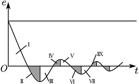
Figure 8. Typical second-order system unit step error curve.

Let $e\left(k\right)$ denote the error value at the current discrete sampling time, and let $e\left(k-1\right)$ and $e\left(k-2\right)$ represent the error values at the previous and second-to-previous sampling times, respectively. It can be obtained that:

$\begin{array}{cc}\hfill & \Delta e\left(k\right)=e\left(k\right)-e\left(k-1\right)\hfill \\ \hfill & \Delta e\left(k-1\right)=e\left(k-1\right)-e\left(k-2\right)\hfill \end{array}(25)$

Based on the error and its variation, the qualitative analysis of the unit step response curve of the second-order system shown in Figure 8 is as follows:

1. When $\left|e\left(k\right)\right|>M_1$, it means that the absolute value of the error is already large. Regardless of the trend of the error change, the controller output should be considered as a constant value output to achieve rapid adjustment of the error, so that the absolute value of the error decreases at the maximum speed while avoiding overshoot. At this point, it is equivalent to implementing open-loop control.

2. When $e\left(k\right)\Delta e\left(k\right)>0$ or $\Delta e\left(k\right)=0$, it indicates that the error is changing in the direction of increasing absolute error value, or the error is a constant value and has not changed.

If $\left|e\left(k\right)\right|⩾M_2$, it indicates that the error is relatively large. It is recommended to consider implementing a stronger control action by the controller to make the absolute value of the error change in the direction of decreasing, rapidly reducing the absolute value of the error. The output of the controller is given by:

$\begin{array}{ll}\hfill u\left(k\right)& =u\left(k-1\right)+k_1\left\{k_p\left[e\left(k\right)-e\left(k-1\right)\right]+k_{i}e\left(k\right)\right.\hfill \\ \hfill & \left.+k_d\left[e\left(k\right)-2e\left(k-1\right)+e\left(k-2\right)\right]\right\}\hfill \end{array}(26)$

If $\left|e\left(k\right)\right|<M_2$, it indicates that although the error is changing in the direction of increasing absolute error value, the absolute value of the error itself is not very large. It is recommended to consider implementing a general control action to reverse the trend of the error, making it change in the direction of decreasing absolute error value. The output of the controller is given by:

$\begin{array}{ll}\hfill u\left(k\right)& =u\left(k-1\right)+k_p\left[e\left(k\right)-e\left(k-1\right)\right]+k_{i}e\left(k\right)\hfill \\ \hfill & +k_d\left[e\left(k\right)-2e\left(k-1\right)+e\left(k-2\right)\right]\hfill \end{array}(27)$

3. When $e\left(k\right)\Delta e\left(k\right)<0,\Delta e\left(k\right)\Delta e\left(k\right)>0$ or $e\left(k\right)=0$, it indicates that the absolute value of the error is changing in the direction of decreasing, or it has reached a steady state. At this point, it is recommended to consider keeping the controller output unchanged.

4. When $e\left(k\right)\Delta e\left(k\right)<0,\Delta e\left(k\right)\Delta e\left(k\right)<0$, it indicates that the error is in a critical state. If the absolute value of the error is large at this time, that is $\left|e\left(k\right)\right|⩾M_2$, stronger control action can be considered, namely:

$u\left(k\right)=u\left(k-1\right)+k_1{k}_p{e}_m\left(k\right)(28)$

If the absolute value of the error is small at this time, that is $\left|e\left(k\right)\right|<M_2$, weaker control action can be considered, namely:

$u\left(k\right)=u\left(k-1\right)+k_2{k}_p{e}_m\left(k\right)(29)$

5. When $\left|e\left(k\right)\right|⩽\epsilon$(precision), it indicates that the absolute value of the error is very small. At this time, adding an integral component can reduce the steady-state error.

In the above formulas, $e_m\left(k\right)$ is the kth extremum of the error e; $u\left(k\right)$ is the output of the controller for the kth time; $u\left(k-1\right)$ is the output of the controller for the (k-1)th time; k₁ > 1 is the gain amplification coefficient, 0 < k₁ < 1; k₂ is the suppression coefficient, 0 < k₂ < 1; M₁, M₂ is the set error limit, M₁ > M₂ > 0; k is the index of the control cycle (a natural number); ɛ is any small positive real number.

In Figure 8, in regions I, III, VII, etc., the error is changing in the direction of decreasing absolute value. At this point, it is recommended to adopt a waiting strategy, which is equivalent to implementing open-loop control. In regions II, IV, VI, VIII, etc., the absolute value of the error is changing in the direction of increasing, and it is recommended to implement stronger or general control actions according to the magnitude of the error to suppress dynamic error.

The PID controller (Liu et al., 2020; Liu and Sui, 2021; Gao and Xiong, 2022) is inherently a single-input single-output system. However, in the case of a robotic arm with six joints, each joint can be considered as an individual output. Consequently, the robotic arm body controller would encompass a total of six inputs and six outputs. Hence, this particular fact was duly considered during the design process of the controller, leading to the appropriate design of its input and output components.

For the input of expert PID controller,

$e\left(k\right)=\sqrt{{\displaystyle \sum _{i=1}^6}erro{r}_i{\left(k\right)}^2}(30)$

$e\left(k\right)$ is the input of the expert PID controller, and $erro{r}_i\left(k\right)$ is the error between the actual angle of each joint motor of the robotic arm and the expected angle solved by the model, i = 1, 2, … , 6.

Increase a proportional factor $P\left(i\right)$ for the output of expert PID controller,

$angl{e}_i\left(k\right)=r_i\left(k\right)+u\left(k\right)*P\left(i\right),i=\mathrm{1,2},\dots ,6(31)$

$u\left(k\right)$ is the output of the expert PID controller; $r_i\left(k\right)$ is the expected angle of each joint of the robotic arm, i = 1, 2, … , 6; $angl{e}_i\left(k\right)$ is the control input angle of each joint motor of the robotic arm, and $P\left(i\right)$ is the proportional factor of the actual error of each joint motor in the input of the expert PID controller, which is calculated as follows:

$P\left(i\right)=\frac{erro{r}_i\left(k\right)}{e\left(k\right)},i=\mathrm{1,2},\dots ,6(32)$

Ultimately, the control system of this six-degree-of-freedom robotic arm is based on kinematic modeling with the addition of an expert PID controller to achieve the control of the end of the robotic arm to quickly and accurately reach the desired position. The structural block diagram of the whole control system is shown in Figure 9.

Figure 9

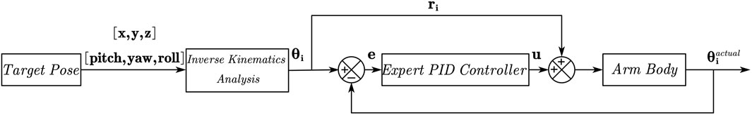
Figure 9. The structure diagram of the six-axis robotic arm control system.

4 Results and discussion

4.1 Results

In this paper, we used the open-source 6-DOF manipulator as the experimental platform. The specific structural parameters of the robotic arm are l₁ = 224mm, l₂ = 224mm, l₃ = 164mm, d₃ = 52.4mm, d₄ = 80.5 mm. By combining the forward and inverse kinematic analyses of the 6-DOF manipulator in Sections 3.1, 3.2, the kinematic model of the 6-DOF manipulator can be established. Based on this kinematic model, experiments were conducted using an expert PID control algorithm to verify the accuracy and stability of the control algorithm.

In order to verify the accuracy and stability of the expert PID control algorithm, the initial position of the 6-DOF manipulator is set as [500, 100, 50] and the initial attitude as [0, 90°, 0]. The 6-DOF manipulator is controlled to run along a straight line, the end position of the straight line is [350, −100, 50], and the attitude of the manipulator is still maintained as [0, 90°, 0]. After the inverse kinematics analysis of the initial pose and target pose of the 6-DOF manipulator, the initial Angle of the six joints is [5.41,-55.77,-69.91,-14.13,90,0], and the target Angle is [-24.22, −91.89, −116.52, −24.63, 90, 0]. The target angles of the six joints were introduced into the control system of the manipulator. The iteration times of the expert PID control algorithm was set to be 300, and each iteration took 0.015s. Joint five remained at 90°and joint six remained at 0°. Finally, the error results from joint one to joint four when the target point is reached are shown in Figure 10.

Figure 10

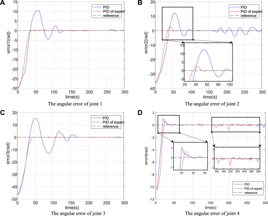
Figure 10. Angular error from joint 1 to joint 4. (A) The angular error of joint 1; (B) The angular error of joint 2; (C) The angular error of joint 3; (D) The angular error of joint 4.

According to Figure 10, the angular error from joint one to joint 4 has a significant variation in the effect of control action under the two control algorithms of classic PID and expert PID. The angular error from joint one to joint four can converge swiftly within 0.75s under the action of the expert PID control algorithm, however, the regulation time of the traditional PID algorithm is slower. Furthermore, the expert PID control algorithm has a lower overshoot than the traditional PID algorithm, with an overshoot of just 6.9% at the maximum, which is decreased by nearly 20% when compared to the traditional PID. At the same time, the expert PID algorithm is more resistant to interference than the traditional PID algorithm, as shown in (b) and (d) of Figure 10. It is clear that the expert PID algorithm outperforms the traditional PID algorithm in terms of control precision and stability.

Subsequently, employing the expert PID control algorithm, we proceeded to execute an experimental endeavor aimed at regulating the movement of the robotic arm along a rectangular trajectory subsequent to traversing a straight line. The end-effector poses of the robotic arm were created by employing a rectangular trajectory generation function. Subsequently, the list of joint angles for the six joints was solved using inverse kinematics. The list is imported into the control system of the robotic arm to obtain the running trajectory of the six-axis robotic arm and the actual angles of the six joint motors during the movement as shown in Figures 11, 12.

Figure 11

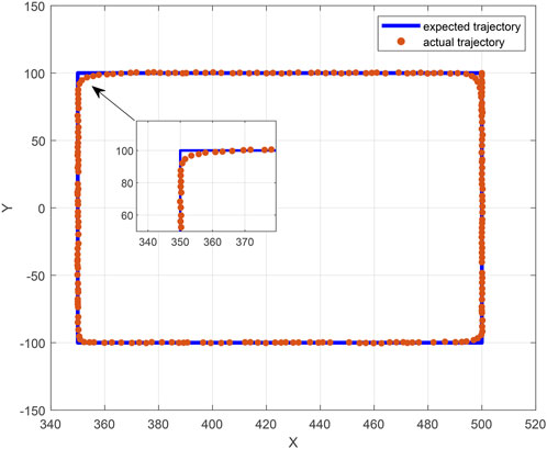
Figure 11. The motion trajectory of the six-axis robotic arm.

Figure 12

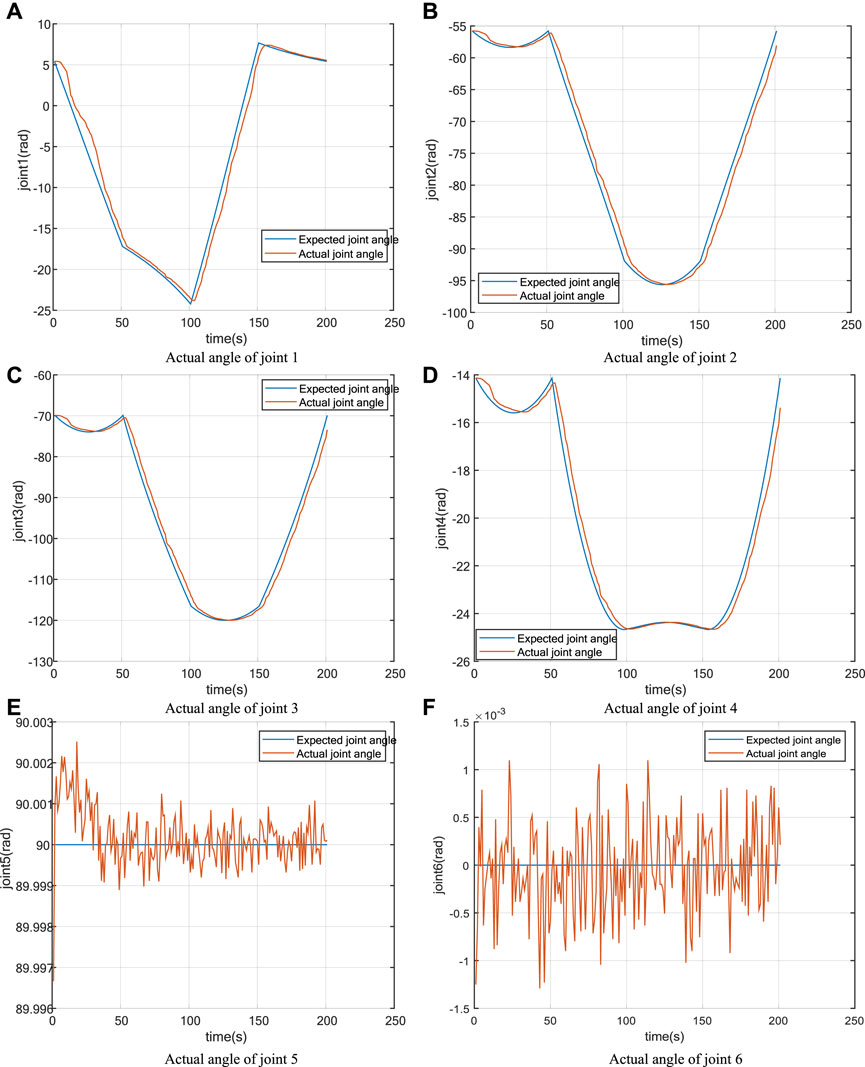
Figure 12. Actual trajectory of the six joints of the robotic arm. (A) Actual angle of joint 1; (B) Actual angle of joint 2; (C) Actual angle of joint 3; (D) Actual angle of joint 4; (E) Actual angle of joint 5; (F) Actual angle of joint 6.

According to Figure 11, the motion trajectory of the robotic arm retains good precision in the straight-line part of the rectangle trajectory when using the expert PID control algorithm. The real motion trajectory is more rounded at the corners than the intended trajectory because the rectangular trajectory generation must be discretized into multiple trajectory points before inverse kinematics solving. Furthermore, there are some hardware problems during robotic arm movement, such as joint motor output inaccuracy and inter-joint friction. As a result, at the corner of the rectangle trajectory, the inaccuracy of the actual motion trajectory is greater than the error of the target motion trajectory. Similarly, in Figure 12, it can be observed that the trajectory tracking from joint one to joint four is very good. The mean error for joint one was 1.152° and the maximum error was 3.373°. The mean error for joint two was 1.326° the maximum error was 2.899°. The mean error for joint three was 1.668° and the maximum error was 4.271°. The mean error for joint four was 0.368° and the maximum error was 1.485°, while joints five and six only wobble slightly around 90° and 0°, with an error size of 0.001° or less.

Subsequently, to validate the efficacy of the expert PID algorithm in governing the motion of the robotic arm along an arc trajectory, a circular trajectory list comprising 800 trajectory points is generated using the trajectory generating function. Subsequently, the position list of the trajectory points is solved kinematically and imported into the control system of the robotic arm. This enables the acquisition of the actual position of the six-degree-of-freedom robotic arm along the circular trajectory, as well as the actual angle of the six joint motors during the process, as depicted in Figures 13, 14.

Figure 13

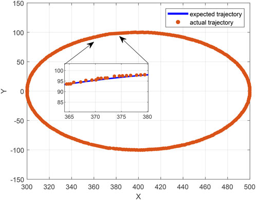
Figure 13. The motion trajectory of the six-axis robotic arm.

Figure 14

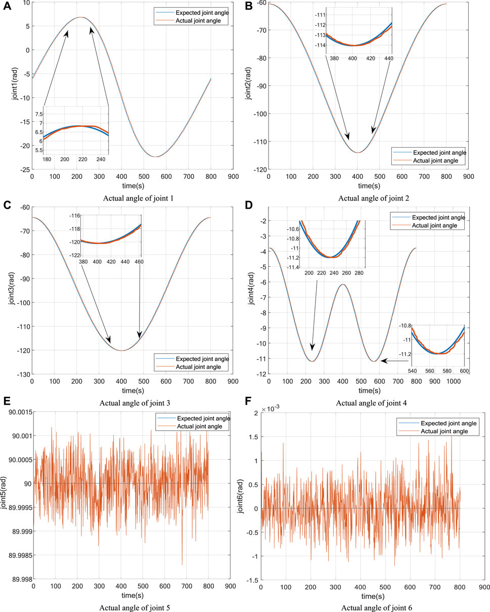
Figure 14. Actual trajectory of the six joints of the robotic arm. (A) Actual angle of joint 1; (B) Actual angle of joint 2; (C) Actual angle of joint 3; (D) Actual angle of joint 4; (E) Actual angle of joint 5; (F) Actual angle of joint 6.

According to the findings presented in Figure 13, it is evident that the expert PID algorithm demonstrates excellent performance in effectively controlling the robotic arm during its movement along a circular trajectory. The algorithm successfully maintains a high level of control accuracy by minimizing the target error to within a few millimeters or even approaching zero. Additionally, Figure 14 illustrates the smooth movement of the joint motors, specifically joints 1 to 4, along the circular trajectory. The trajectory tracking is highly effective. The mean error for joint 1 was 0.223° and the maximum error was 0.579°. The mean error for joint 2 was 0.393° and the maximum error was 0.763°. The average error for joint 3 was 0.396° and the maximum error was 0.809°. The average error for joint 4 was 0.084° and the maximum error was 0.174°. Furthermore, joints 5 and 6 exhibit a stable orientation with minor oscillations within the range of 90° and 0°.

4.2 Discussion

However, there are still a lot of flaws and shortcomings in our robotic arm motion control experiment since the robotic arm is subject to model error, outside interference, and other real-world issues. In future research, we will incorporate the dynamics model of the robotic arm into the control system and implement moment compensation. This entails utilising a combination of kinematic control and dynamics compensation to enhance the speed and accuracy of controlling the robotic arm. Meanwhile, sensors such as torque sensors and position sensors can be attached to the robotic arm’s end to ensure the model’s correctness and precision while also reducing model error.

5 Conclusion

This study constructs a physical verification platform for the control algorithm of the manipulator, with the goal of improving the manipulator’s accuracy and response time in the complicated power plant environment. Firstly, we build a kinematic model based on the robot’s geometric structure. Then, we utilise CAN communication to enable the upper computer software to operatethe the six-degree-of-freedom robotic arm. Secondly, an expert PID controller is designed to improve the traditional PID controller, which makes the 6-DOF manipulator more stable and more accurate in the course of trajectory operation. Finally, after comparing the two experimental results, we discover that the expert PID algorithm has a faster response speed in the control of the manipulator than the traditional PID algorithm. The expert PID algorithm can converge quickly within 0.75s, and the overshoot is smaller, with a maximum of only 6.9%. In addition, the expert PID control algorithm also shows good control effect in the subsequent rectangular and circular trajectory tracking experiments. Furthermore, the robotic arm’s control algorithm appears to be more effective in tracking the relative circular motion.

Data availability statement

The original contributions presented in the study are included in the article/Supplementary Material, further inquiries can be directed to the corresponding author.

Author contributions

WJ: Funding acquisition, Project administration, Resources, Supervision, Writing–review and editing. XW: Conceptualization, Data curation, Formal Analysis, Investigation, Methodology, Software, Validation, Visualization, Writing–original draft. ZL: Supervision, Writing–review and editing.

Funding

The author(s) declare financial support was received for the research, authorship, and/or publication of this article. This research was supported by the Foundation of Shanghai Institute of Technology (Grant number: XTCX2021-10).

Acknowledgments

Thanks to XW for obtaining the experimental results through numerous experiments and analyzing the results to complete the first draft of the paper. We would like to thank WJ for providing the hardware platform for this experimental project and supervising and guiding the whole experimental process. We also thank ZL for writing guidance and revising the manuscript.

Conflict of interest

The authors declare that the research was conducted in the absence of any commercial or financial relationships that could be construed as a potential conflict of interest.

Publisher’s note

All claims expressed in this article are solely those of the authors and do not necessarily represent those of their affiliated organizations, or those of the publisher, the editors and the reviewers. Any product that may be evaluated in this article, or claim that may be made by its manufacturer, is not guaranteed or endorsed by the publisher.

Supplementary material

The Supplementary Material for this article can be found online at: https://www.frontiersin.org/articles/10.3389/fenrg.2024.1367903/full#supplementary-material

References

Alhassan, A. B., Zhang, X., Shen, H., and Xu, H. (2020). Power transmission line inspection robots: a review, trends and challenges for future research. Int. J. Electr. Power Energy Syst. 118, 105862. doi:10.1016/j.ijepes.2020.105862

CrossRef Full Text | Google Scholar

Alkayyali, M., and Tutunji, T. A. (2019). “Pso-based algorithm for inverse kinematics solution of robotic arm manipulators,” in 2019 20th International Conference on Research and Education in Mechatronics (REM), Wels, Austria, 23-24 May 2019, 1–6. doi:10.1109/REM.2019.8744103

CrossRef Full Text | Google Scholar

Almusawi, A. R., Dülger, L. C., and Kapucu, S. (2016). A new artificial neural network approach in solving inverse kinematics of robotic arm (denso vp6242). Comput. Intell. Neurosci. 2016, 1–10. doi:10.1155/2016/5720163

CrossRef Full Text | Google Scholar

Bodie, K., Tognon, M., and Siegwart, R. (2021). Dynamic end effector tracking with an omnidirectional parallel aerial manipulator. IEEE Robotics Automation Lett. 6, 8165–8172. doi:10.1109/lra.2021.3101864

CrossRef Full Text | Google Scholar

Borase, R. P., Maghade, D. K., Sondkar, S. Y., and Pawar, S. N. (2021). A review of pid control, tuning methods and applications. Int. J. Dyn. Control 9, 818–827. doi:10.1007/s40435-020-00665-4

CrossRef Full Text | Google Scholar

Dai, Y., Gao, H., Yu, S., and Ju, Z. (2022). A fast tube model predictive control scheme based on sliding mode control for underwater vehicle-manipulator system. Ocean. Eng. 254, 111259. doi:10.1016/j.oceaneng.2022.111259

CrossRef Full Text | Google Scholar

Djaneye-Boundjou, O., Xu, X., and Ordóñez, R. (2022). “Automated particle swarm optimization based pid tuning for control of robotic arm,” in 2016 IEEE National Aerospace and Electronics Conference (NAECON) and Ohio Innovation Summit (OIS), Dayton, OH, USA, 25-29 July 2016, 164–169. doi:10.1109/NAECON.2016.7856792

CrossRef Full Text | Google Scholar

Dou, R., Yu, S., Li, W., Chen, P., Xia, P., Zhai, F., et al. (2022). Inverse kinematics for a 7dof humanoid robotic arm with joint limit and end pose coupling. Mech. Mach. Theory 169, 104637. doi:10.1016/j.mechmachtheory.2021.104637

CrossRef Full Text | Google Scholar

Gan, J. Q., Oyama, E., Rosales, E. M., and Hu, H. (2005). A complete analytical solution to the inverse kinematics of the pioneer 2 robotic arm. Robotica 23, 123–129. doi:10.1017/S0263574704000529

CrossRef Full Text | Google Scholar

Gao, H., and Xiong, L. (2022). Research on a hybrid controller combining rbf neural network supervisory control and expert pid in motor load system control. Adv. Mech. Eng. 14, 168781322211099. doi:10.1177/16878132221109994

CrossRef Full Text | Google Scholar

Guan, D., Yang, N., Lai, J., Siu, M. F. F., Jing, X., and Lau, C. K. (2021). Kinematic modeling and constraint analysis for robotic excavator operations in piling construction. Automation Constr. 126, 103666. doi:10.1016/j.autcon.2021.103666

CrossRef Full Text | Google Scholar

Guida, R., De Simone, M. C., Dašić, P., and Guida, D. (2019). Modeling techniques for kinematic analysis of a six-axis robotic arm. IOP Conf. Ser. Mater. Sci. Eng. 568, 012115. doi:10.1088/1757-899X/568/1/012115

CrossRef Full Text | Google Scholar

Hayat, A. A., Chittawadigi, R. G., Udai, A. D., and Saha, S. K. (2013). Identification of denavit-hartenberg parameters of an industrial robot. Identif. Denavit-Hartenberg Param. Industrial Robot. doi:10.1145/2506095.2506121

CrossRef Full Text | Google Scholar

Iqbal, J., Tahir, A. M., and ul Islam, R. (2012). “Robotics for nuclear power plants–challenges and future perspectives,” in 2012 2nd international conference on applied robotics for the power industry (CARPI) (IEEE), Zurich, Switzerland, 11-13 September 2012, 151–156.

Google Scholar

Krishna, S., and Vasu, S. (2018). Fuzzy pid based adaptive control on industrial robot system. Mater. Today Proc. 5, 13055–13060. doi:10.1016/j.matpr.2018.02.292

CrossRef Full Text | Google Scholar

Liu, J., Li, T., Zhang, Z., and Chen, J. (2020). Narx predictionbased parameters online tuning method of intelligent pid system. IEEE Access 8, 130922–130936. doi:10.1109/access.2020.3007848

CrossRef Full Text | Google Scholar

Liu, X., and Sui, T. (2021). Expert control of mine hoist control system. Wirel. Commun. Mob. Comput. 2021, 1–8. doi:10.1155/2021/5592351

PubMed Abstract | CrossRef Full Text | Google Scholar

Long, T., Li, E., Hu, Y., Yang, L., Fan, J., Liang, Z., et al. (2021). A vibration control method for hybrid-structured flexible manipulator based on sliding mode control and reinforcement learning. IEEE Trans. Neural Netw. Learn. Syst. 32, 841–852. doi:10.1109/TNNLS.2020.2979600

PubMed Abstract | CrossRef Full Text | Google Scholar

Lu, S., Zhang, Y., and Su, J. (2017). Mobile robot for power substation inspection: a survey. IEEE/CAA J. Automatica Sinica 4, 830–847. doi:10.1109/jas.2017.7510364

CrossRef Full Text | Google Scholar

Menendez, O., Cheein, F. A. A., Perez, M., and Kouro, S. (2017). Robotics in power systems: Enabling a more reliable and safe grid. IEEE Ind. Electron. Mag. 11, 22–34. doi:10.1109/mie.2017.2686458

CrossRef Full Text | Google Scholar

Meng, X., He, Y., and Han, J. (2019). “Hybrid force/motion control and implementation of an aerial manipulator towards sustained contact operations,” in 2019 IEEE/RSJ International Conference on Intelligent Robots and Systems (IROS) (IEEE), Macau, China, 03-08 November 2019, 3678–3683.

CrossRef Full Text | Google Scholar

Parra-Vega, V., Arimoto, S., Yun-Hui, L., Hirzinger, G., and Akella, P. (2003). Dynamic sliding pid control for tracking of robot manipulators: theory and experiments. IEEE Trans. Robotics Automation 19, 967–976. doi:10.1109/tra.2003.819600

CrossRef Full Text | Google Scholar

Peng, J., Yang, Z., Wang, Y., Zhang, F., and Liu, Y. (2019). Robust adaptive motion/force control scheme for crawler-type mobile manipulator with nonholonomic constraint based on sliding mode control approach. ISA Trans. 92, 166–179. doi:10.1016/j.isatra.2019.02.009

PubMed Abstract | CrossRef Full Text | Google Scholar

Qin, L., Liu, F., Liang, L., and Gao, J. (2014). Fuzzy adaptive robust control for space robot considering the effect of the gravity. Chin. J. Aeronautics 27, 1562–1570. doi:10.1016/j.cja.2014.10.023

CrossRef Full Text | Google Scholar

Shamseldin, M. A. (2021). Optimal covid-19 based pd/pid cascaded tracking control for robot arm driven by bldc motor. Wseas Trans. Syst. 20, 217–227. doi:10.37394/23202.2021.20.24

CrossRef Full Text | Google Scholar

Srivastava, S., Gupta, M., Prasannakumar, N., Rudola, A., Mallick, A., et al. (2018). A comparative study of pid and neuro-fuzzy based control schemes for a 6-dof robotic arm. J. Intelligent Fuzzy Syst. 35, 5317–5327. doi:10.3233/JIFS-169814

CrossRef Full Text | Google Scholar

Wang, L., Chai, T., and Zhai, L. (2009). Neural-network-based terminal sliding-mode control of robotic manipulators including actuator dynamics. IEEE Trans. Industrial Electron. 56, 3296–3304. doi:10.1109/TIE.2008.2011350

CrossRef Full Text | Google Scholar

Xiao, J., Han, W., and Wang, A. (2017). “Simulation research of a six degrees of freedom manipulator kinematics based on matlab toolbox,” in 2017 International Conference on Advanced Mechatronic Systems (ICAMechS), Xiamen, China, 06-09 December 2017, 376–380. doi:10.1109/ICAMechS.2017.8316502

CrossRef Full Text | Google Scholar

Xiao, W., Chen, K., Fan, J., Hou, Y., Kong, W., and Dan, G. (2023). Ai-driven rehabilitation and assistive robotic system with intelligent pid controller based on rbf neural networks. Neural Comput. Appl. 35, 16021–16035. doi:10.1007/s00521-021-06785-y

CrossRef Full Text | Google Scholar

Xu, K., and Wang, Z. (2023). The design of a neural network-based adaptive control method for robotic arm trajectory tracking. Neural Comput. Appl. 35, 8785–8795. doi:10.1007/s00521-022-07646-y

CrossRef Full Text | Google Scholar

Yu, X. (2020). Hybrid-trajectory based terminal sliding mode control of a flexible space manipulator with an elastic base. Robotica 38, 550–563. doi:10.1017/S0263574719000857

CrossRef Full Text | Google Scholar

Zhang, T., and Dai, J. (2021). Electric power intelligent inspection robot: a review. J. Phys. Conf. Ser. IOP Publ. 1750, 012023. doi:10.1088/1742-6596/1750/1/012023

CrossRef Full Text | Google Scholar

Zhang, Y., and Yan, P. (2019). Adaptive observer-based integral sliding mode control of a piezoelectric nano-manipulator. IET Control Theory and Appl. 13, 2173–2180. doi:10.1049/iet-cta.2018.6192

CrossRef Full Text | Google Scholar

Zhao, G., Jiang, D., Liu, X., Tong, X., Sun, Y., Tao, B., et al. (2022). A tandem robotic arm inverse kinematic solution based on an improved particle swarm algorithm. Front. Bioeng. Biotechnol. 10, 832829. doi:10.3389/fbioe.2022.832829

PubMed Abstract | CrossRef Full Text | Google Scholar

Zhonglin, Z., Bin, F., Liquan, L., and Encheng, Y. (2021). Design and function realization of nuclear power inspection robot system. Robotica 39, 165–180. doi:10.1017/s0263574720000740

CrossRef Full Text | Google Scholar