 Xianglong Zhang
 Chuang Zhou2
 Shufeng Dong
95% of researchers rate our articles as excellent or good
Learn more about the work of our research integrity team to safeguard the quality of each article we publish.
Find out more
ORIGINAL RESEARCH article
Front. Energy Res. , 19 June 2024
Sec. Smart Grids
Volume 12 - 2024 | https://doi.org/10.3389/fenrg.2024.1366859
Under the background of “dual carbon” strategy, the integration of renewable energy adds volatility to the grid. Relying solely on generation-side resources for regulation is inadequate, necessitating a flexible demand response from diverse demandside resources. This paper employs a physical connection and information exchange between the distribution network and microgrids to leverage the advantages of centralized-distributed optimization. This establishes a coordinated demand response model between the distribution network and microgrids, gradually establishing a new type of distribution network that integrates interconnected grids and microgrids. This also necessitates the analysis of the response characteristics of various load resources within microgrids and the categorization and modeling of loads based on their response speeds. Additionally, a method for evaluating the multi-time scale schedulable capacity of microgrids is proposed. Finally, a coordinated demand response model between the distribution network and microgrids based on the schedulable capacity assessment is established. This model is validated through case studies, demonstrating its effectiveness. The coordinated demand response between distribution networks and microgrids enables them to operate in a collaborative and economically safe manner.
The global market is becoming more interconnected due to societal demand and the shift in global industrial development. As a result, climate change and environmental pollution have become increasingly severe issues. The consumption of non-renewable resources in an outdated pattern leads to excessive depletion of finite resources and serious environmental pollution, which constitutes an unsustainable development model. Therefore, the energy transition is currently undergoing continuous experimentation as a strategic approach capable of achieving both improved environmental conditions and resource sustainability (Gielen et al., 2019; Hillerbrand et al., 2019; Li and Kong, 2019).
In China, the power industry accounts for about 40% of the country’s carbon emissions (Kang et al., 2022). Under the background of “double carbon,” carbon reduction in the power industry has become a key task (Li Y. W. et al., 2022; Zhang and Kang, 2022; Huang et al., 2023). Opening up new energy and low-carbon transformation is an inevitable trend in the development of the power system. With the continuous improvement of the whole industrial chain system of new energy in China, the construction cost of new energy development has been declining, the pace of market-oriented development of wind power and photovoltaic generation has been accelerating, and the proportion of new energy has gradually increased. At the same time, the impact of uncertain factors such as climate and seasons on new energy generation has brought many new challenges to the power system (Wei, 2019; Li P. S. et al., 2021; Chen, 2021; Yuan et al., 2022; Zhou et al., 2023). It is necessary to fully tap into the diverse resources on the demand side and form a more flexible, convenient, and rapid demand response to improve the regulating capacity of the power system (Jiang, 2018; Gan, 2022).
Microgrids can provide an effective solution to the problems of difficult distributed resource management and insufficient power grid regulation capacity caused by new energy access (Ju and Chen, 2023; Belkhier and Oubelaid, 2024). At the same time, demand response guides users to actively shift and avoid peak loads through market-oriented means (Xu et al., 2018; Wang et al., 2020), which effectively reduce peak loads while also obtaining certain economic benefits for users. It is a win–win approach for the power grid and users.
Demand response is mainly classified into two types: price-based and incentive-based. At present, in the practical application of demand response, users spontaneously adjust their electricity consumption behavior based on the electricity price to obtain benefits from the peak valley dispersion. Large-scale users can obtain corresponding incentives by signing contracts with the power grid to complete the agreed peak load shifting response within the agreed time period. Cui et al. (2021) built the demand response model and guided load adjustments using a price elasticity matrix to alleviate peak system pressures. Li W. et al. (2021) proposed an incentive mechanism for load aggregation merchants targeting shiftable load resources from the perspective of user electricity preferences, thus obtaining optimal incentive contracts for users and optimal scheduling strategies for load aggregation merchants. Both of the above methods fail to closely integrate users’ response with grid-side regulation needs, so the response effect often fails to meet expectations. Peak-valley prices are difficult to accurately and dynamically reflect regulation needs, and the scale and frequency of the latter are relatively limited (Fan et al., 2022). For users, the response cost is high and it is difficult to form scale benefits.
Assessing demand response potential is an important aspect of demand response research, also known as the schedulable capacity or controllable capacity. Currently, research on the demand response potential assessment has made some progress (Li et al., 2017; Xu et al., 2017; Zhang et al., 2018), with three typical assessment methods: electricity consumption analysis, elasticity coefficient method, and regression analysis method. Alvarez et al. (2004) quantified the quality and characteristics of its demand response resources through electricity consumption analysis at higher education institutions, achieving a demand response potential assessment at both intraday and intraday time scales. Li et al. (2017) analyzed the range of load response for industrial, commercial, and residential users based on the electricity demand-price elasticity coefficient, combined with industry load characteristics statistical models, forming a demand response potential envelope. Kong et al. (2022) established a secondary regression parameter database for typical electricity consumption patterns by analyzing key factors influencing power users’ participation in demand response, proposing a depth-subdomain adaptive demand response potential assessment method based on feature similarity. The elasticity coefficient assessment method primarily targets load group behaviors with a certain magnitude and is not related to the actual specific load response process. The regression analysis method focuses on users with regular electricity consumption patterns, studying the characteristics and patterns of their historical responses to assess their demand response potential. Both of these methods cannot be used to guide users in conducting demand response.
In addition to theoretical research, countries around the world are actively implementing demand response in practice. The United States has established demand response based on electricity markets in various states, with a wide range of demand response types and relatively well-developed policies and regulations, placing it in a leading position globally. The European Union has not yet formed a comprehensive demand response implementation plan. However, European countries have launched distinctive demand response projects tailored to their national conditions. For instance, France has implemented the “Red, White, and Blue Electricity Price” policy to encourage user participation in demand response. In the United Kingdom, market participants primarily include large electricity users and load aggregation merchants, with transactions executed every half hour and participation in the United Kingdom's electricity balancing mechanism (Huang and Zhang, 2020).
Microgrids not only optimize the coordination of local generation, load, and storage resources to enhance regional economic benefits but also participate as controllable units in the optimization and scheduling at the distribution network level. They provide services such as peak shaving, frequency regulation, and demand response, thereby enhancing grid regulation capabilities and further improving the reliability and flexibility of power system operations (Yang et al., 2014; Dashtdar et al., 2022). Currently, the main application scenarios for coordinated distribution–microgrid operations are optimization and scheduling. Osama et al. (2020) divided large distribution networks into multiple virtual microgrids and proposed a microgrid optimization design method that includes distributed generation units, thereby optimizing the operation and control of the distribution network. Zhou and Ai (2020) studied distribution network systems with multiple microgrids, introducing the concept of a virtual coordinator to divide the topology into a “component–subsystem–main system” structure, achieving a joint economic dispatch of the distribution network and multiple microgrids. Yan et al. (2021) proposed a two-pole network constraint equivalent energy interaction method for multiple microgrids, ensuring flexible connectivity and power exchange between microgrids while maintaining the privacy of microgrids and the operational safety of the distribution network.
As an independent demand-side stakeholder, microgrid-related research studies on the demand response characteristics are relatively well-established, with some explorations and innovations in coordinated distribution-microgrid demand response. Li X. et al. (2022) considered various types of microgrid demand response characteristics and proposed a distributed optimization scheduling strategy for urban distribution systems, reducing overall operating costs and improving the economic viability of microgrids and distribution systems. Li Z. K. et al. (2022) introduced a dual-layer scheduling model considering microgrid demand response and power exchange, with the lower layer coordinating the outputs of various microgrids to minimize operating costs, while the upper layer optimizes active and reactive power at the distribution network level. Kahnamouei and Lotfifard (2022) achieved a critical load recovery after extreme events through the coordinated optimization of distributed energy sources, microgrids, and demand response.
However, current research studies have not fully utilized the function of distribution networks as guideline for the demand response of microgrids nor has it distinguished the demand response of microgrids from other stakeholders at the practical application level. If the guidance role of the distribution network on microgrid demand response can be strengthened, forming a dedicated channel for coordinated demand response between distribution and microgrids, where microgrid demand response becomes the execution of “demand response instructions” from the distribution network, it can achieve more targeted and frequent small-scale demand response. Additionally, it would exhibit characteristics of being more stable, accurate, and rapid in response.
Therefore, this paper conducts research on the distribution–microgrid-coordinated demand response based on the multi-time scale schedulability assessment. Conducting specific application scenario research on coordinated distribution–microgrid demand response, this paper aims to enhance the rapid regulation capabilities of distribution networks through scaled and normalized microgrid demand response, thereby forming a hierarchical demand response structure. The contributions of this study are as follows:
(1) Proposed a load grading modeling method based on the response time of loads. By considering the different response characteristics of different loads within the microgrid, especially their response time during demand response, a load grading modeling method was proposed. The grading of loads corresponds to demand response at multiple time scales.
(2) Introduced a multi-time scale dispatching ability assessment method for microgrids. Based on the grading model, demand response was divided into four scales: day-ahead, hourly, minute-level, and second-level. A multi-time scale dispatching ability assessment model for microgrids was established to describe the relationship between schedulable loads and corresponding costs.
(3) Studied distribution–microgrid coordinated demand response based on the multi-time scale schedulable capacity assessment. Leveraging the load grading model and multi-time scale schedulable capacity assessment of microgrids, a distribution–microgrid coordinated demand response framework was developed. This framework maximizes the advantages of centralized-distributed optimization, allowing rapid instructions from the distribution network to the microgrid for stable and accurate responses. This approach achieves stable and efficient demand response while maximizing economic benefits.
First, the response time, sustainability time, response uncertainty, and differential characteristics of demand response of commonly available demand response loads are studied, and the load is divided into seven levels according to response time, as shown in Figure 1. Different levels of load resources can meet the regulatory needs of different scenarios. Below is a load modeling of interruptible loads, energy storage, electric vehicles, and air conditioning that this article focuses on, and a brief explanation of their control methods of how they involve in demand response.
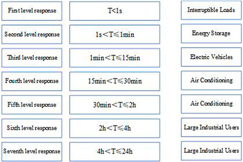
Figure 1. Load grading by response time.
Interruptible loads can be controlled through load control devices such as specialized transformer load control terminal or precise load control terminal to achieve shunt tripping function and complete load control. The response time is less than 1 s, and it belongs to the first-level response resources.
where
The energy storage can flexibly adjust the charge–discharge power according to the power command, achieving a bidirectional power flow and fast response. The response time is in the second level, so the energy storage belongs to the second-level response resources. Then, a load model for energy storage is established:
where
The electric vehicles can be regarded as the user’s private and movable energy storage. To achieve a two-way power flow, special charging station equipment is required and complex practical factors such as ownership, battery loss, financial compensation, and user willingness are considered. More technical and policy supports are needed in the actual application; therefore, this paper only considered the charging properties of electric vehicles which conducted demand response by stopping charging. The response time is approximately 5–15 min, which belongs to the third-level response resources.
User j could choose to accept a set of charging interruption periods, denoted as
where
Air conditioning is a typical temperature-controlled load, and its operation characteristics are closely related to the thermal changes in buildings. Buildings have certain thermal storage properties, and human comfort temperature is within a range, which gives air conditioning loads a virtual energy storage property. The temperature adjustment lag makes the response time of air conditioning in the order of hours, making it a fourth- or fifth-level response resource. Then, a load model for air conditioning is established:
where
The dispatching ability of a microgrid refers to the relationship between the reduction amount and corresponding cost in a specific future time period based on the planned/current operating state of the microgrid (Wang, 2020; Xu, 2021). Depending on the time scale, it can be categorized into day-ahead, hourly, minute, and second dispatching abilities.
The evaluation process of the multi-time scale dispatching ability of a microgrid and its specific application scenarios are illustrated in Figure 2.
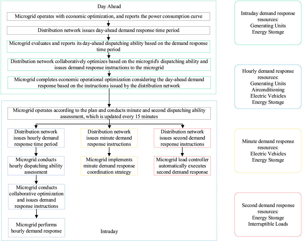
Figure 2. Process flowchart of demand response in the distribution–microgrid based on multi-time scale scalable capability evaluation.
At the day-ahead time scale, the microgrid conducts economic optimization based on time-of-use electricity prices to meet the energy demand of users to the greatest extent. Only the generation units and energy storage output are optimized, and the planned electricity consumption curve is reported to the distribution network. The distribution network then issues day-ahead demand response periods based on the overall situation. The microgrid evaluates its day-ahead dispatching ability for demand response periods and reports it to the distribution network. Day-ahead demand response ensures the energy demand of users and is achieved solely through generation units and energy storage resources. The distribution network performs coordinated optimization based on the dispatching ability of each microgrid and issues demand response instructions to each microgrid. The microgrid then conducts day-ahead optimization, considering the demand response based on the instructions.
At the intraday time scale, the microgrid operates normally based on the day-ahead optimization results while conducting minute and second dispatching ability evaluations, which are updated every 15 min. When the distribution network issues hourly demand response periods, the microgrid evaluates its hourly dispatching ability for the specific period and reports it to the distribution network. Hourly demand response sacrifices a portion of user satisfaction with energy consumption and involves not only generation units and energy storage resources but also air conditioning and electric vehicles. After coordinated optimization by the distribution network, demand response instructions are issued to the microgrid, and the microgrid performs hourly demand response accordingly. When the distribution network issues minute-level demand response instructions, the microgrid executes pre-set minute-level demand response coordination strategies, which are achieved through electric vehicles and energy storage with minute-level response speeds. When the distribution network issues second-level demand response instructions, the microgrid’s load controller automatically executes the corresponding instructions, involving interruptible loads and energy storage with second-level response speeds.
In summary, different time scales of demand response involve different resources. The day-ahead grid side has more diverse regulation measures, so the microgrid side participates in day-ahead demand response while meeting the energy needs of users, utilizing generation units and energy storage as response resources. For the overall grid, the dispatchable day-ahead resources are relatively limited. Therefore, the microgrid sacrifices a portion of users’ satisfaction to increase the response quantity, mobilizing all resources that can meet the response speed for intraday demand response. Hourly demand response involves generation units, air conditioning, electric vehicles, and energy storage. A minute-level demand response involves electric vehicles and energy storage. The second-level demand response only considers energy storage and interruptible loads.
The economic optimization results of microgrid operation in the day-ahead grid size are used as the basis for dispatching ability evaluation. Every day is divided into
where
where
where
where
The power balance constraint, generation unit output and ramping constraints, equipment constraints, and environmental temperature constraints in the microgrid are expressed as follows from Eq. 19 to Eq. 22:
(1) Power balance constraint:
where
(2) Generation unit output and ramping constraints:
where
(3) Equipment constraints:>Eqs 1–14
(4) Environmental temperature constraints:
where
Day-ahead dispatching ability (DADA) refers to the relationship between the achievable reduction amount and the corresponding cost in the known day-ahead demand response time period
where
Step 1: Perform day-ahead economic optimization to obtain the microgrid’s daily operating cost without considering the demand response, denoted as
Step 2: Add the reduction amount constraint to the microgrid’s economic operation optimization problem in Section 2.1, as shown in the following Eq. 24:
where
Step 3: The decision variables are the microgrid’s purchasing power and the output of generation units and energy storage. Solve the optimization problem.
Step 4: If the optimization problem has a solution, obtain the microgrid’s daily operating cost
Step 5: Based on the obtained
Hourly dispatching ability (HDA) refers to the relationship between the achievable reduction amount and the corresponding cost in the hourly demand response time period
The parameters in the equation have the same meanings as in the day-ahead dispatching ability, and the solution steps are also the same as in the day-ahead evaluation method, so it will not be repeated. The final result is a set of data denoted as
where
(1) Environmental temperature cost:
where
(2) Electric vehicle compensation:
where
Minute dispatching ability (MDA) refers to the relationship between the achievable reduction amount and the corresponding cost in the minute-level demand response for a microgrid. The expression for MDA is given by Eq. 30:
The solution steps and the evaluation methods are consistent with the previous approach and will not be reiterated. The differences are as follows: 1) instead of solving for specific time periods, the solution will be for the 1-h time period 30 min later, with updates every 15 min; 2) the power generation units and air conditioning load will remain in their planned operating state without control adjustments, and the optimization decision variables will be the energy storage output and the binary variable
The second dispatching ability refers to the maximum reduction amount that a microgrid can achieve in second-level demand response, without considering costs. The calculation method is as follows in Eqs 31–33:
where
When the distribution network issues a second-level demand response instruction, the load controller within the microgrid automatically executes the corresponding instruction. It disconnects the interruptible loads and simultaneously initiates the discharge of the energy storage system at the maximum discharge power until it reaches
At the day-ahead level, the distribution network receives the power consumption plan curve
The objective function is to minimize the operating cost of the distribution network and the interaction cost between the distribution network and the microgrid. The decision variables are the power generation output of the units and the demand response quantity of the microgrid. The objective function can be expressed as follows in Eqs 34–37:
where
(1) Distribution network electricity procurement cost:
where
(2) Distribution network generation cost:
where
(3) Interactions cost between the distribution network and microgrid:
where
The power balance constraint of the distribution network, line flow constraints, unit output and ramping constraints, and reduction amount constraints are expressed as follows Eqs 38–43:
(1) Power balance constraints:
where
(2) Line-flow constraints:
where
(3) Unit output and ramping constraints:
where
(4) Reduction amount constraints:
where
By solving the above optimization problem, we can obtain the reduction amount
During the minute demand response coordinated between the distribution network and microgrid, considering the requirement for response speed, the reported dispatching ability of microgrid
During a second demand response coordinated between the distribution network and microgrid, the reported second dispatching ability by the microgrid is denoted as
The calculations will be performed on a computer with an Intel Core i7-12700 2.10 GHz processor and 16 GB of memory. The programming language used will be MATLAB R2019a, and the CPLEX 12.10 solver will be invoked for solving the optimization problem.
The evaluation and analysis of the dispatchable capacity at different time scales were conducted for Microgrid 1 during the time period of 15:00–17:00. Figure 3 presents the economic operation results of Microgrid 1 in advance. The various regions of time-of-use electricity prices are indicated by dashed lines and colors at the bottom of the x-axis. The green color represents the off-peak electricity price periods, the red color represents the peak electricity price periods, and the white color represents the high peak electricity price periods.
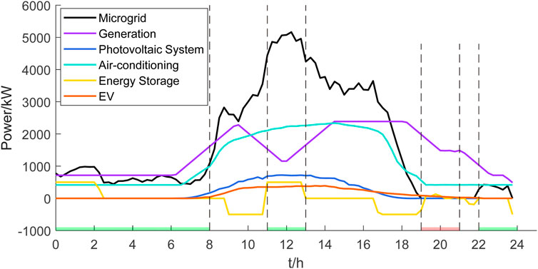
Figure 3. Day-ahead economic operation curve of Microgrid 1.
It can be observed that the time period of 11:00–13:00 corresponds to the off-peak electricity price, during which the output of the microgrid units is reduced, the energy storage system is in the charging state, and the power purchased by the microgrid is at its peak. The time period of 19:00–21:00 corresponds to the peak electricity price, during which the microgrid itself has a relatively small electricity consumption and achieves internal electricity balance through the units and a small amount of energy storage. The time periods of 8:00–11:00 and 13:00–19:00 both correspond to the high peak electricity price, and the microgrid has a relatively large electricity consumption during these periods. The units have a higher output, and the energy storage system has a negative value, indicating that it is in the discharging state to reduce the amount of electricity purchased by the microgrid. The total cost of the advance economic operation of the microgrid is 48,761.45 yuan, including 27,428.32 yuan for purchased electricity and 21,049.98 yuan for generation costs.
Figure 4 illustrates the operation of Microgrid 1 with a demand response reduction of 600 kW in advance. The red dashed line indicates the demand response period from 15:00 to 17:00. It can be observed that the day-ahead demand response is achieved through the units and energy storage. During the demand response period, the output of the units increases and the energy storage system starts discharging, thereby reducing the power purchased by the microgrid. At this time, the operating cost of the microgrid is 48,794.29 yuan, which is slightly higher compared to the pre-planned cost.
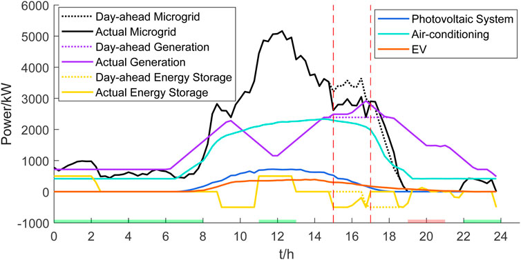
Figure 4. Day-ahead demand response reduction of 600 kW of Microgrid 1.
Table 1 presents the relationship between the day-ahead demand response reduction and cost for Microgrid 1. It can be observed that as the reduction amount increases, the cost of purchased electricity decreases, while the generation cost increases. At this point, the unit cost of generation is higher than the unit cost of purchased electricity, resulting in an overall increase in the total cost. The maximum demand response reduction for Microgrid 1 during the time period of 15:00–17:00 is 680 kW.
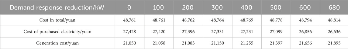
Table 1. Relationship between day-ahead demand response reduction and cost of Microgrid 1.
Figure 5 illustrates the operation of Microgrid 1 with an hourly demand response reduction of 1,000 kW. The resources involved in the hourly demand response include units, air conditioning, electric vehicles, and energy storage. As the reduction amount increases, the microgrid first utilizes the energy storage with the lowest cost and starts discharging. Then, the units increase their output. Finally, the electric vehicles and air conditioning, which have higher response costs, are adjusted. The electric vehicles stop charging, and the air conditioning adjusts its output within a small range based on the characteristics of the energy storage.
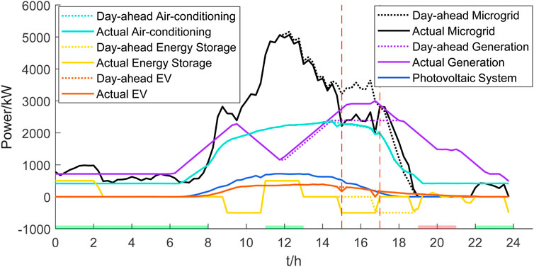
Figure 5. Hourly demand response reduction of 1,000 kW of Microgrid 1.
Table 2 presents the relationship between the hourly demand response reduction and cost for Microgrid 1. It can be observed that as the reduction amount increases, the cost of purchased electricity and generation initially increases, then decreases, and finally increases again. The decrease in the middle is caused by the response of electric vehicles. When the electric vehicles stop charging, the electricity consumption of the microgrid decreases, resulting in a reduction in both the cost of purchased electricity and generation. The maximum hourly demand response reduction for Microgrid 1 during the time period of 15:00–17:00 is 1,080 kW.
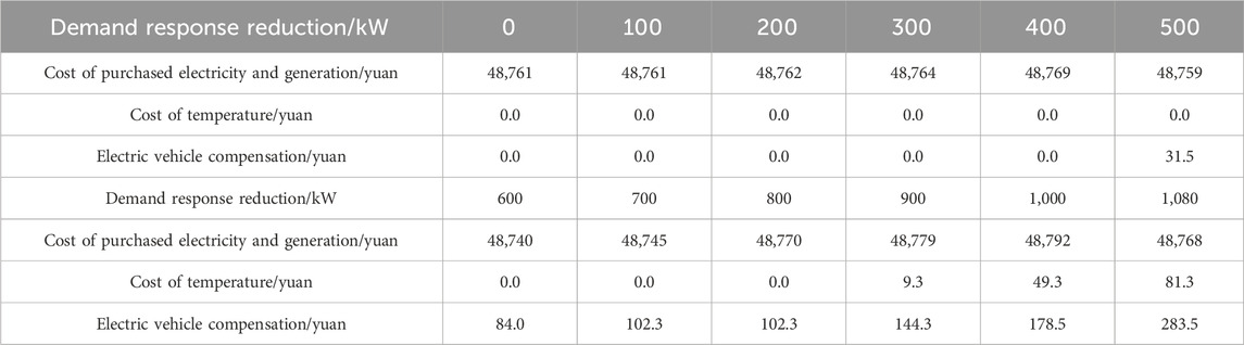
Table 2. Relationship between hourly demand response reduction and cost of Microgrid 1.
Figure 6 illustrates the operation of Microgrid 1 with a minute demand response reduction of 700 kW. The resources involved in the minute demand response are electric vehicles and energy storage. The energy storage discharges, and the electric vehicles stop charging.
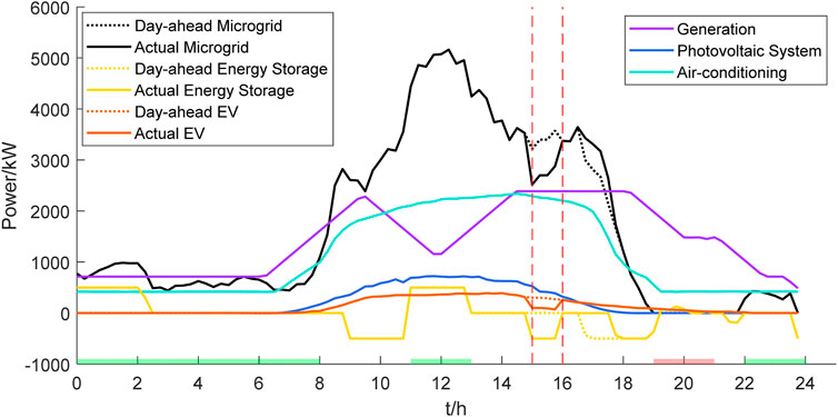
Figure 6. Minute demand response reduction of 700 kW of Microgrid 1.
Table 3 presents the relationship between the minute demand response reduction and cost for Microgrid 1. As the reduction amount increases, the response from electric vehicles gradually increases, and the compensation from electric vehicles also increases. The maximum minute demand response reduction for Microgrid 1 during the time period of 15:00–17:00 is 760 kW.
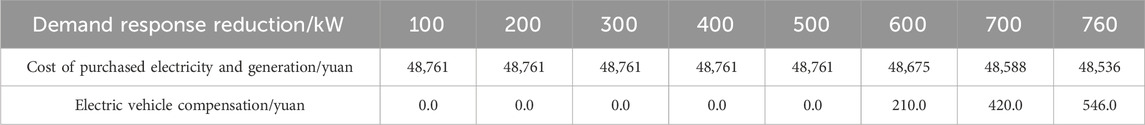
Table 3. Relationship between minute demand response reduction and the cost of Microgrid 1.
Figure 7 illustrates the relationship between the demand response reduction and the corresponding cost increase at multiple time scales for Microgrid 1. It can be observed that there are certain similarities in the demand response across the three time scales. When the reduction amount is less than 500 kW, the cost increase is minimal. However, after the reduction amount exceeds 500 kW, the cost increase shows a clear upward trend.
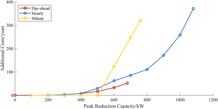
Figure 7. Curve of relationship between multi-time scale demand response reduction and cost of Microgrid 1.
In addition to these similarities, there are also some differences. In the advance time scale, the dispatchable capacity is relatively small, resulting in lower response costs compared to the hourly scale. In the hourly scale, there is a greater availability of dispatchable resources and a larger dispatchable capacity. However, this additional capacity comes at the expense of user satisfaction, resulting in relatively higher costs. In the minute scale, the first 500-kW reduction is provided by energy storage with almost no cost. However, the subsequent 260-kW reduction is provided by electric vehicles, resulting in higher costs.
Figures 8–10 represent the day ahead, hourly, and minute dispatching abilities of three microgrids during the time period of 15:00–17:00. These abilities correspond to the relationship between the reduction amount and cost increase. According to the parameters in Supplementary Table SA3, it can be observed that in terms of microgrid loads and various resource magnitudes, Microgrid 2 > Microgrid 1 > Microgrid 3. Correspondingly, at various time scales, the maximum dispatchable capacity of the microgrids follows the order Microgrid 2 > Microgrid 1 > Microgrid 3, as indicated in Table 4. When the reduction quantity is small, the dispatch costs of each microgrid are relatively low. However, with an increase in the reduction quantity, the costs of each microgrid start to rise. Additionally, the marginal dispatch cost becomes larger, and there is a turning point in the reduction quantity, with Microgrid 2 > Microgrid 1 > Microgrid 3.
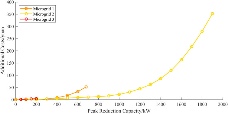
Figure 8. Day-ahead scheduling capability of the microgrid.
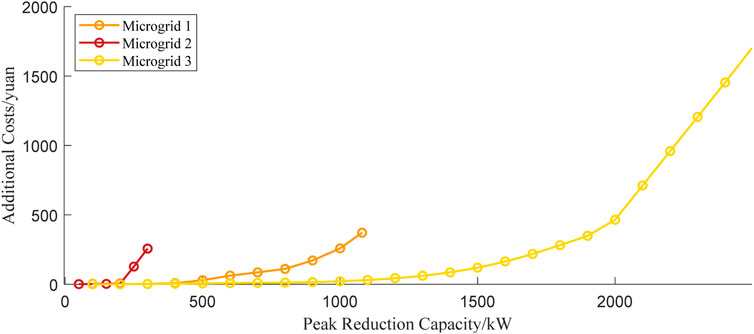
Figure 9. Hourly scheduling capability of the microgrid.

Figure 10. Minute scheduling capability of the microgrid.
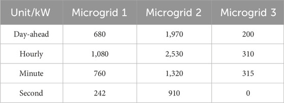
Table 4. Maximum schedulable capacity of the microgrid with multiple time scales.
The hourly level is taken as an example to illustrate the process of demand response between distribution and microgrids. When the distribution network meets the safety constraints of the line and receives instructions from superiors to reduce peak load during the 15:00–17:00 period, only the unit peak load cost of each microgrid is considered. When the peak shaving instructions are 1 MW, 2 MW, and 3 MW, the reduction amounts of microgrid 1, 2, and 3 obtained by solving are shown in Table 5, making the total adjustment cost of the three microgrids the lowest. At this point, the microgrids participating in demand response have similar reduction unit prices. The schedulability of the microgrid is composed of several straight lines between the reduction amount and cost, but in reality, there is not a strict linear relationship. Therefore, the reduction unit prices are not completely consistent, and the error is within an acceptable range.
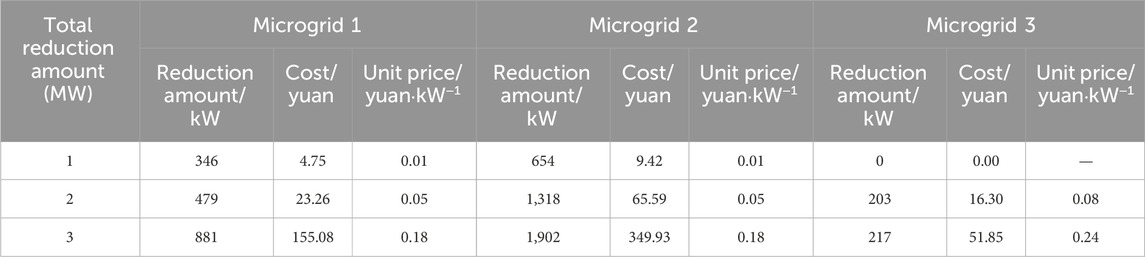
Table 5. Microgrid peak shaving command and corresponding cost.
When the total reduction amount is 3 MW, the demand response curves for the three microgrids are shown in Figures 11–13.
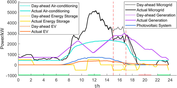
Figure 11. Demand response reduction of 881 kW of Microgrid 1.
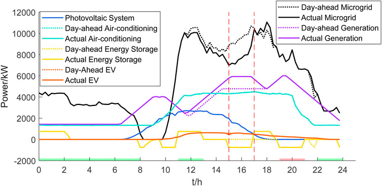
Figure 12. Demand response reduction of 1,902 kW of Microgrid 2.
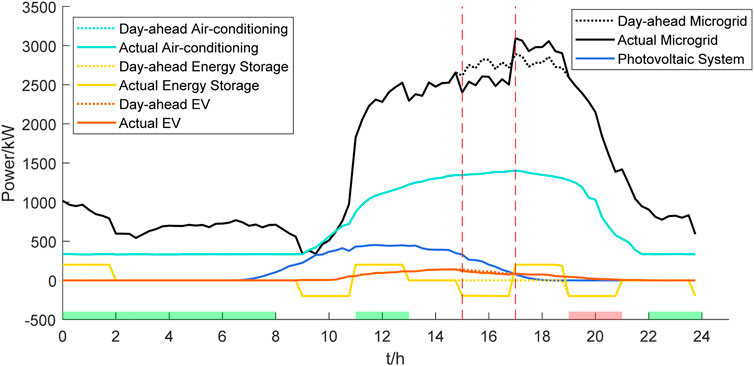
Figure 13. Demand response reduction of 217 kW of Microgrid 3.
Taking the hourly scale as an example, the process of demand response in distribution–microgrid coordination is explained. When the distribution network operates within the constraints of line safety and receives instructions from the higher-level authority to implement peak shaving during the time period of 15:00–17:00, the focus is on the unit peak shaving cost of each microgrid.
To improve the scale and frequency of demand response implementation, this paper proposes a coordinated demand response method for distribution–microgrid based on the multi-time scale dispatchable capacity assessment. It is hoped that coordinating distribution and microgrids in a collaborative demand response architecture can enhance the guidance role of the distribution grid in responding to microgrid demands. Simultaneously, microgrid control strategies should be improved to enable more stable, efficient, and accurate responses, reinforcing the proactive support role of microgrids in the distribution grid. The multi-time scale dispatchable capacity refers to the relationship between the achievable load adjustment and the corresponding cost for demand response at different time scales, including day-ahead, hourly, minute, and second levels. The following conclusion can be drawn:
(1) Different resources are mobilized for demand response at different time scales based on the response characteristics of various load resources. Day-ahead demand response mainly considers the response characteristics of demand-side units and energy storage while meeting the user’s energy demand. Hourly demand response, in addition to units and energy storage, also mobilizes air conditioning and electric vehicle resources at the expense of sacrificing some user’s energy satisfaction. Minute-level demand response mobilizes load resources with fast response characteristics such as energy storage and electric vehicles. The second-level demand response corresponds to energy storage and interruptible loads.
(2) The maximum adjustable power and unit adjustment cost at different time scales in the microgrid are different. The overall trend of the maximum adjustable power is as follows: hourly > day-ahead > minute > second; the overall trend of unit adjustment cost is second > minute > hourly > day-ahead, which is consistent with the characteristics of demand response at different time scales.
(3) Through the dispatchable capacity assessment, the distribution network has a clear understanding of the adjustable amount and corresponding cost for each microgrid. With the distribution–microgrid-coordinated demand response architecture, the distribution network can quickly issue instructions, and the microgrid can respond stably and accurately according to the instructions. The coordinated method enables more targeted and frequent demand response on a smaller scale while ensuring the safety constraints of the lines and achieving the lowest total adjustment cost for the microgrid.
However, there are directions for further improvement and enrichment.
(1) Uncertainty in new energy/load forecasting accuracy. The paper currently fully considers the response characteristics of various adjustable resources within the microgrid but does not take into account the impact of factors such as the volatility, randomness, and accuracy of load forecasting on the assessment of microgrid schedulable capacity.
(2) Long-term schedulable capacity assessment. Currently, only the schedulable capacity of microgrids for intraday and intraday is evaluated, without consideration of longer time scales such as “monthly” and “annually.” Evaluation of the schedulable capacity within these time frames can have an impact on grid planning.
The raw data supporting the conclusion of this article will be made available by the authors, without undue reservation.
ZX: writing–original draft and writing–review and editing. ZC: writing–original draft and writing–review and editing. HY: writing–original draft and writing–review and editing. DS: writing–original draft and writing–review and editing.
The author(s) declare financial support was received for the research, authorship, and/or publication of this article. The project was supported by the State Grid Corporation of China (No. 5108-202356049A-1-1-ZN). The funder was not involved in the study design, collection, analysis, interpretation of data, the writing of this article, or the decision to submit it for publication.
The authors sincerely acknowledge the contribution of all individuals, reviewers, and editors for their contribution toward the production of this manuscript.
Author ZX was employed by State Grid Economic and Technological Research Institute Co., Ltd.
The remaining authors declare that the research was conducted in the absence of any commercial or financial relationships that could be construed as a potential conflict of interest.
All claims expressed in this article are solely those of the authors and do not necessarily represent those of their affiliated organizations, or those of the publisher, the editors, and the reviewers. Any product that may be evaluated in this article, or claim that may be made by its manufacturer, is not guaranteed or endorsed by the publisher.
The Supplementary Material for this article can be found online at: https://www.frontiersin.org/articles/10.3389/fenrg.2024.1366859/full#supplementary-material
Alvarez, C., Gabaldon, A., and Molina, A. (2004). Assessment and simulation of the responsive demand potential in end-user facilities application to a university customer. IEEE Trans. Power Syst. 19 (2), 1223–1231. doi:10.1109/tpwrs.2004.825878
Belkhier, Y., and Oubelaid, A. (2024). Novel design and adaptive coordinated energy management of hybrid fuel-cells/tidal/wind/PV array energy systems with battery storage for microgrids. Energy Storage e556. doi:10.1002/est2.556
Chen, Y. (2021) Scheduling strategy of power system considering demand response uncertainties. Master Thesis. China: South China University of Technology.
Cui, Y., Xiu, Z. G., Liu, C., Zhao, Y. T., Tang, Y. H., Chai, X. Z., et al. (2021). Dual level optimal dispatch of power system considering demand response and pricing strategy on deep peak regulation. Proc. CSEE 41 (13), 185–193. doi:10.13334/j.0258-8013.pcsee.202105
Dashtdar, M., Belkhier, Y., Bajaj, M., Sadegh, S. M., Belik, M., and Rubanenko, O. (2022). “Protection of DC microgrids based on frequency domain analysis using fourier transform,” in 2022 IEEE 3rd KhPI Week on Advanced Technology (KhPIWeek), Kharkiv, Ukraine, October, 2022, 1–6.
Fan, S., Wei, Y. H., He, G. Y., and Li, Z. Y. (2022). Discussion on demand response mechanism for new power systems. Automation Electr. Power Syst. 46 (07), 1–12. doi:10.7500/AEPS20210726010
Gan, Z. T. (2022) Multi-objective scheduling optimization of power system considering demand response under carbon neutral background. Master Thesis. China: North China Electric Power University.
Gielen, D., Boshell, F., Saygin, D., Bazilian, M. D., Wagner, N., and Gorini, R. (2019). The role of renewable energy in the global energy transformation. Energy Strategy Rev. 24, 38–50. doi:10.1016/j.esr.2019.01.006
Hillerbrand, R., Milchram, C., and Schippl, J. (2019). The Capability Approach as a normative framework for technology assessment: capabilities in assessing digitalization in the energy transformation. TATuP-Z. Für Tech. Theor. Und Prax./J. Technol. Assess. Theory Pract. 28, 52–57. doi:10.14512/tatup.28.1.52
Huang, M. H., Tang, K. J., Dong, S. F., Nan, B., and Song, Y. H. (2023). Optimal power flow considering user-side carbon emission allowances based on carbon flow theory. Power Syst. Technol. 47 (07), 1–10. doi:10.13335/j.1000-3673.pst.2023.0028
Huang, R., and Zhang, S. F. (2020). Practice and enlightenment of power demand-side management in major developed countries. J. North China Electr. Power Univ. 6, 47–55. doi:10.14092/j.cnki.cn11-3956/c.2020.06.006
Jiang, X. K. (2018) Power system optimal operation with large-scale wind power and electric vehicle integrated considering demand response. Master Thesis. China: Huazhong University of Science and Technology.
Ju, Y. T., and Chen, X. (2023). Distributed active and reactive power coordinated optimal scheduling of networked microgrids based on two-layer multi-agent reinforcement learning. Proceeding CSEE 42 (23), 1–16. doi:10.13334/j.0258-8013.pcsee.212737
Kahnamouei, A., and Lotfifard, S. (2022). Enhancing resilience of distribution networks by coordinating microgrids and demand response programs in service restoration. IEEE Syst. J. 16 (2), 3048–3059. doi:10.1109/jsyst.2021.3097263
Kang, C. Q., Du, E. S., Li, Y. W., Zhang, N., Chen, Q. X., Guo, H. Y., et al. (2022). Key scientific problems and research framework for carbon perspective research of new power systems. Power Syst. Technol. 46 (03), 821–833. doi:10.13335/j.1000-3673.pst.2021.2550
Kong, X. Y., Liu, C., Wang, C. S., Li, S. W., and Chen, S. S. (2022). Demand response potential assessment method based on deep subdomain adaptation network. Proceeding CSEE 42 (16), 5786–5797+6156. doi:10.13334/j.0258-8013.pcsee.210903
Li, P. S., Wu, Z. J., Zhang, C., Hu, M. Q., Li, S. F., Wang, F. S., et al. (2021a). Distributed hybrid-timescale voltage/var control in active distribution networks. Automation Electr. Power Syst. 45 (16), 160–168. doi:10.7500/AEPS20201225004
Li, W., Han, R. D., Sun, C. J., Fu, P., Zhang, J., Wang, C., et al. (2021b). An optimal incentive contract and strategy of shiftable loads participation in demand response based on user electricity preference. Proc. CSEE 41 (S1), 4403–4415. doi:10.13334/j.0258-8013.pcsee.202593
Li, X., Ji, H. S., Zhang, R. F., Jiang, T., Chen, H. H., Ning, R. X., et al. (2022b). Distributed optimal scheduling of urban distribution system considering response characteristics of multi-type microgrids. Automation Electr. Power Syst. 46 (17), 74–82. doi:10.7500/AEPS20220226002
Li, Y. H, and Kong, L. (2019). Developing solar and wind power generation technology to accelerate China’s energy transformation. Bull. Chin. Acad. Sci. 34, 426–433. doi:10.16418/j.issn.1000-3045.2019.04.007
Li, Y. W., Zhang, N., Du, E. S., Liu, Y. L., Cai, X., He, D. W., et al. (2022a). Mechanism study and benefit analysis on power system low carbon demand response based on carbon emission flow. Proc. CSEE 42 (08), 2830–2842. doi:10.13334/j.0258-8013.pcsee.220308
Li, Z. K., Wang, X. X., Shi, S. S., and Zhang, Z. Q. (2022c). Bi-level optimal dispatch of distribution network considering power interaction among microgrids. South. Power Syst. Technol. 16 (09), 107–118. doi:10.13648/j.cnki.issn1674-0629.2022.09.013
Li, Z. Y., Wang, G., Ding, M. S., and Wang, L. J. (2017). Demand response potential quantitative evaluation considering load statistical characteristics. China Sci. Pap. 12 (05), 529–536. doi:10.3969/j.issn.2095-2783.2017.05.010
Osama, R. A., Zobaa, A. F., and Abdelaziz, A. Y. (2020). A planning framework for optimal partitioning of distribution networks into microgrids. IEEE Syst. J. 14 (1), 916–926. doi:10.1109/jsyst.2019.2904319
Wang, B. B., Yang, X. C., and Yang, S. C. (2015). Demand response performance and potential system dynamic analysis based on the long and medium time dimensions. Proc. CSEE 35 (24), 6368–6377. doi:10.13334/j.0258-8013.pcsee.2015.24.012
Wang, X. C. (2020) Research on evaluation method of industrial demand response capacity. Master Thesis. China: Zhejiang University.
Wang, Y. Q., Qiu, J., Tao, Y. C., and Zhao, J. H. (2020). Carbon-oriented operational planning in coupled electricity and emission trading markets. IEEE Trans. Power Syst. 35 (4), 3145–3157. doi:10.1109/tpwrs.2020.2966663
Wei, B. R. (2019) Research on power system optimal dispatch considering demand response and optimization methods. Master Thesis. China: Guangxi University.
Xu, C. S. (2021) Research on Integrated demand response of industrial park. Master Thesis. China: Zhejiang University.
Xu, Q. S., Ding, Y. F., Yan, Q. G., and Zheng, A. X. (2017). Research on evaluation of scheduling potentials and values on large consumers. Proc. CSEE 37 (23), 6791–6800. doi:10.13334/j.0258-8013.pcsee.162638
Xu, Z., Sun, H. B., and Guo, Q. L. (2018). Review and prospect of integrated demand response. Proceeding CSEE 38 (24), 7194–7205+7446. doi:10.13334/j.0258-8013.pcsee.180893
Yan, M. Y., Shahidehpour, M., Paaso, A., Zhang, L. X., Alabdulwahab, A., and Abusorrah, A. (2021). Distribution network-constrained optimization of peer-to-peer transactive energy trading among multi-microgrids. IEEE Trans. Smart Grid 12 (2), 1033–1047. doi:10.1109/tsg.2020.3032889
Yang, X. F., Su, J., Lv, Z. P., Liu, H. T., and Li, R. (2014). Overview on micro-grid technology. Proc. CSEE 34 (01), 57–70. doi:10.13334/j.0258-8013.pcsee.2014.01.007
Yuan, B., Zhang, T. X., and Wang, Y. F. (2022). Study on electric power system operational decision-making with consideration of large scale user load directrix demand response. Water Resour. Hydropower Eng. 53 (12), 150–159. doi:10.13928/j.cnki.wrahe.2022.12.016
Zhang, X., Hug, G., Kolter, J. Z., and Harjunkoski, I. (2018). Demand response of ancillary service from industrial loads coordinated with energy storage. IEEE Trans. Power Syst. 33 (1), 951–961. doi:10.1109/tpwrs.2017.2704524
Zhang, Z. G., and Kang, C. Q. (2022). Challenges and prospects for constructing the new-type power system towards a carbon neutrality future. Proc. CSEE 42 (08), 2806–2819. doi:10.13334/j.0258-8013.pcsee.220467
Zhou, F. Q., Wang, J., Zhao, X. D., and Deng, L. C. (2023). Innovate and optimize power demand response to support the construction of new power system. Power Demand Side Manag. 25 (01), 1–4. doi:10.3969/j.issn.1009-1831.2023.01.001
Keywords: carbon peaking and carbon neutrality goals, distribution and microgrid cooperation, demand response, multi-time scale, load classification, scheduling capability
Citation: Zhang X, Zhou C, Hua Y and Dong S (2024) Research on distribution–microgrid-coupled network demand response based on a multi-time scale. Front. Energy Res. 12:1366859. doi: 10.3389/fenrg.2024.1366859
Received: 07 January 2024; Accepted: 30 April 2024;
Published: 19 June 2024.
Edited by:
Salvatore Favuzza, University of Palermo, ItalyReviewed by:
Matteo Manganelli, Italian National Agency for New Technologies, Energy and Sustainable Economic Development (ENEA), ItalyCopyright © 2024 Zhang, Zhou, Hua and Dong. This is an open-access article distributed under the terms of the Creative Commons Attribution License (CC BY). The use, distribution or reproduction in other forums is permitted, provided the original author(s) and the copyright owner(s) are credited and that the original publication in this journal is cited, in accordance with accepted academic practice. No use, distribution or reproduction is permitted which does not comply with these terms.
*Correspondence: Shufeng Dong, ZG9uZ3NodWZlbmdAemp1LmVkdS5jbg==
Disclaimer: All claims expressed in this article are solely those of the authors and do not necessarily represent those of their affiliated organizations, or those of the publisher, the editors and the reviewers. Any product that may be evaluated in this article or claim that may be made by its manufacturer is not guaranteed or endorsed by the publisher.
Research integrity at Frontiers
Learn more about the work of our research integrity team to safeguard the quality of each article we publish.