Optimization of multi-vehicle obstacle avoidance based on improved artificial potential field method with PID control

In the context of multi-vehicle formation, obstacle avoidance in unknown environments presents a number of challenges, including obstacles near the target, susceptibility to local minima, and dynamic obstacle avoidance. To address these issues in multi-vehicle formation control and obstacle avoidance within unknown environments, this paper uses PID control to optimize the potential field function of the artificial potential field method and conducts simulation experiments. The results demonstrate that the proposed algorithm achieves reductions of 39.7%, 41.9%, 24.8% and 32.0% in four efficiency functions (total iteration times, formation efficiency function value, energy consumption and standard deviation of iteration times) compared to other algorithms. The improved algorithm more effectively addresses the challenge of slow obstacle avoidance when vehicles approach the target and can handle unexpected situations such as local minima and dynamic obstacles. It achieves energy-efficient optimization for multi-vehicle obstacle avoidance in complex environments.

1 Introduction

In the backdrop of global energy shortages and the adverse impacts on the ecological environment, the automotive industry is rapidly shifting towards new energy, intelligence, and energy-efficient directions. New energy vehicles, characterized by their intelligence, energy efficiency, and environmentally friendly, pollution-free features, have become the primary focus of the future automotive industry. There is an increasing emphasis on the research and utilization of new energy, with active promotion of new energy vehicle projects, leading to a swift expansion of the market. Currently, new energy vehicles in the market primarily rely on electric power, significantly reducing dependence on gasoline, thus lowering environmental pollution and meeting daily commuting needs. In this trend, through the implementation of intelligent technology, vehicles have achieved path planning, obstacle avoidance optimization, enhancing travel efficiency, and notably achieving energy-saving goals. This intelligent development not only makes new energy vehicles more efficient in energy utilization but also enhances driving safety and comfort, laying a solid foundation for the sustainable development of the future automotive industry.

With the development of robot technology and the promotion of social demand, people’s expectation for robots is no longer limited to a single individual, but more and more attention is paid to the system composed of multiple robots. This change is not only due to the fact that complex tasks often exceed the capabilities of a single robot. In practical applications, the cost and time required to develop a single robot are relatively high, while building a multi-robot system is more economical, efficient and time-saving. This is because multi-robot systems, through mechanisms such as resource sharing and batch production, can effectively reduce overall costs, making them more economical in practical applications. With the rise of robot production line, people’s demand for robots has gradually changed from a single individual to a multi-robot system that can work autonomously and cooperatively (Dahiya et al., 2023).

In recent years, scholars have carried out extensive research in the field of multi-vehicle formation control (Oh et al., 2015), focusing on the key aspects of formation establishment, maintenance, switching, obstacle avoidance, adaptive process and so on (Wang et al., 2023). Multi-vehicle formation control aims to achieve collaborative operations among vehicles, forming an organized structure to accomplish specific tasks or achieve particular objectives. In view of the advantages and disadvantages of different formation strategies, two or even more than three formation strategies are usually combined in the formation research to effectively improve the overall performance of the formation system. Among them, the main algorithms used in formation obstacle avoidance are leader-follower method and artificial potential field method. In the leader-follower approach, typically, one vehicle is chosen as the leader, responsible for guiding the entire formation; the remaining vehicles act as followers, adjusting their positions based on specific strategies or algorithms to maintain the formation shape and performance. However, the leader-follower method has a shortcoming, that is, the formation system relies too much on the leader and is almost completely dominated by the leader, which leads to its poor robustness. As shown in Figure 1, the traditional artificial potential field method also has some inherent problems (Fan et al., 2020): (A) Goal Not Reachable or Not Obtainable (GNRON); (B) Trapped in a Local Minimum Region; (C) Obstacle avoidance in dynamic environment.

FIGURE 1

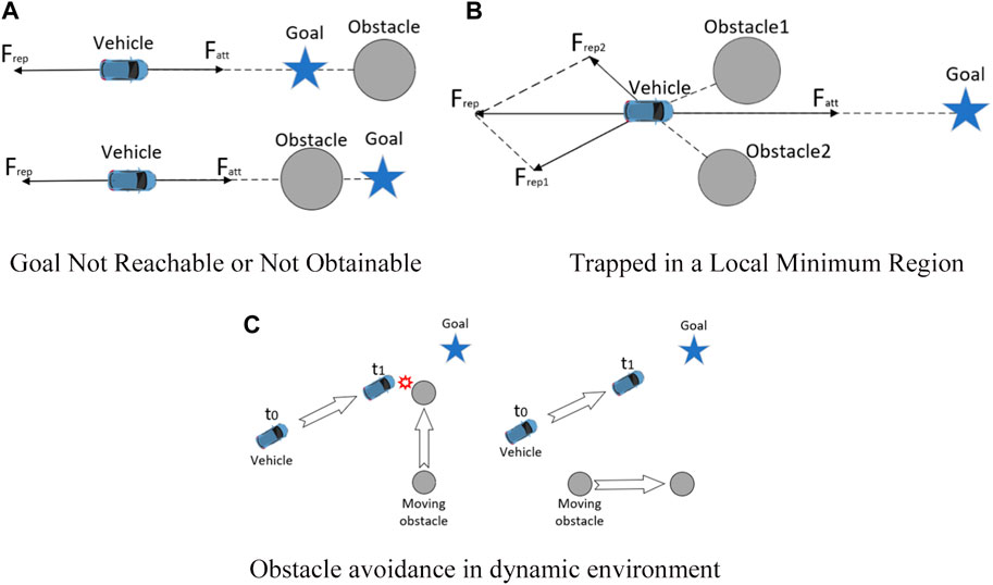
FIGURE 1. Problems of traditional algorithms. (A) Goal Not Reachable or Not Obtainable (B) Trapped in a Local Minimum Region (C) Obstacle avoidance in dynamic environment.

In order to address the issue of goal not reachable or not obtainable of nearby obstacles, several approaches have been proposed in the literature. Jia and Wang (2010) increased the gradient of the attractive potential function around the target to eliminate the GNRON problem. Yang et al. (2016) introduced an additional potential field using the potential filling method in this region. Sfeir et al. (2011) proposed a new repulsive potential field that does not require prior knowledge of the environment. Zhang (2018) revised the definition of the repulsion field by employing a water flow field coordinate system.

To overcome being trapped in a local minimum region during navigation, Matoui et al. (2019) utilized a non-minimum speed algorithm. Sun et al. (2019) applied the dynamic window method to resolve local minimum problems. Xian-Xia et al. (2018) introduced a sector partition method that added virtual obstacles in an appropriate range around the local minimum point. Li et al. (2012) defined the potential function and established a virtual local target. Wu et al. (2023) combined the simulated annealing algorithm and deterministic annealing strategy to help robots escape local minimum points.

To address obstacle avoidance in dynamic environment, Montiel et al. (2015) introduced the concept of parallel evolutionary artificial potential fields. Cheng et al. (2015) proposed an algorithm that combines velocity synthesis and artificial potential fields. Cao et al. (2014) applied the limit cycle theory to multi-vehicle obstacle avoidance and successfully overcame the limitations of the artificial potential field method in vehicle obstacle avoidance control. Zheng et al. (2022) presented a formation method based on a fuzzy artificial potential field approach, effectively solving the problem of multi-vehicle formation control and obstacle avoidance in dynamic environments.

While previous studies primarily focused on limited environmental conditions, they often neglected the complexity and variability of environmental factors. Furthermore, the literature needs more extensive research on unknown obstacle environments, multi-vehicle formation maintenance, and parameter optimization. Considering these gaps, this paper proposes a multi-vehicle obstacle avoidance optimization algorithm based on PID control and an improved artificial potential field function. The algorithm is evaluated using four commonly used efficiency functions: total iteration times of formation obstacle avoidance, formation efficiency function value, energy consumption and standard deviation of iteration times. The simulation results demonstrate that compared to other algorithms, the proposed approach outperforms them in terms of these three efficiency functions (by approximately 30%). It effectively addresses the GNRON problem, alleviates speed problems (both too small and too large), and achieves energy-efficient obstacle avoidance in complex environments.

2 Improvements based on artificial potential field method

In the artificial potential field method (Khatib, 1985), the gravitational gain coefficient (k_att) and repulsive gain coefficient (k_rep) play a crucial role in determining the effectiveness of obstacle avoidance. However, selecting these coefficients is typically based on empirical experience, which may not necessarily be the optimal choice for the given environment. Consequently, this can give rise to various issues, such as the emergence of local minima, longer obstacle avoidance paths, and challenges in obstacle avoidance in dynamic environments. Additionally, other challenges have been encountered in practical applications. Therefore, in the following sections, we aim to enhance the classical artificial potential field method based on existing research in order to address these concerns. This includes introducing PID control in the process of improving the gravitational function, incorporating a velocity-repulsion function based on the position-repulsion function, and innovating the approach to random perturbations.

2.1 Improvement of gravitational function

2.1.1 Improvements to long-distance gravity

In scenarios where the vehicle’s map is significantly large and the target point is far away, the gravity formula indicates that gravity is directly proportional to the distance. Consequently, the gravity force becomes considerably strong, while repulsion force remains relatively small. As a result, the robot is prone to colliding with obstacles during its movement. To mitigate this issue, an optimization can be achieved by modifying the gravitational function. Specifically, when the robot is far away from the target point, the gravitational force should be reduced, and the degree of reduction should be correlated with the distance.

Define the target distance difference e in Eq. 1:

$e=\left\{\begin{array}{l}{q}_o-q_{g}ifleader\\ q_i-q_{\mathrm{e}}iffollower\end{array}\right.(1)$

In the proposed approach, several key variables are utilized: q_o represents the leader’s current position, q_g is the leader’s target position; q_i denotes the follower’s current position, q_e represents the follower’s target position. Notably, the target position of the leader is predetermined, whereas the target position of the follower is the anticipated position based on maintaining the formation corresponding to the leader’s current position.

The enhanced gravitational potential field formula is presented as Eq. 2:

$U_{att}\left(e\right)=\left\{\begin{array}{l}\frac{1}{2}{k}_{att}{e}^2,e\le d\\ d{k}_{att}e-\frac{1}{2}{k}_{att}{d}^2,e>d\end{array}\right.(2)$

where U_att(e) represents the gravitational potential field; k_att is a gravitational gain coefficient greater than 0; d is the given constant, in this case the distance factor.

The corresponding gravitational function is given in Eq. 3:

$F_{att}\left(e\right)=-▽U_{att}\left(e\right)=\left\{\begin{array}{l}{k}_{att}e,e\le d\\ -d{k}_{att}\frac{e}{\parallel e\parallel },e>d\end{array}\right.(3)$

2.1.2 Improvement of gravitational function by PID control

When the agent approaches the target position, the gravitational force is relatively small. If obstacles are present near the target location, the repulsive force might exceed the gravitational force. This leads to prolonged iteration times and difficulties in reaching the goal. To address these challenges, the gravitational function can be further enhanced by incorporating PID control techniques.

The improved gravitational function is given in Eq. 4:

$F_{att}\left(e\right)=k_{p}e+k_i{\int }_0^{t}edt+k_d\frac{\mathrm{d}e}{\mathrm{d}t}(4)$

where k_p, k_i and k_d represent the proportional, integral, and derivative coefficients of the PID control, respectively. These coefficients correspond to the proportional, integral, and derivative items of the distance difference between the vehicle’s current position and the target position.

The above formula represents the continuous expression of PID control, and the discrete form is expressed as shown in Eq. 5:

$F_{att}\left(e_i\right)=k_p{e}_i+k_i{\displaystyle \sum _{i=1}^N}{e}_i+k_d\left(e_i-e_{i-1}\right)(5)$

In the discrete formulation, the proportional term represents the distance difference in the current iteration, while the integral term is the accumulated sum of the distance differences throughout the iteration process. In practical applications, it is not necessary to accumulate the integral term from the initial iteration. In this study, the distance differences of the last 10 iterations are summed. Incorporating the cumulative integral term with the distance ensures that the vehicle’s speed does not become excessively low as it approaches the target. Simultaneously, the differential term accounts for the difference in position difference between the current and previous iterations. This differential term enables the vehicle to execute obstacle avoidance maneuvers in the face of unexpected situations, such as confronting local minima or encountering dynamic obstacles.

2.1.3 Improved gravitational function

Combining the two improvements of 2.1.1 and 2.1.2, the improved gravitational function is obtained as shown in Eq. 6:

$F_{att}\left(e_i\right)=\left\{\begin{array}{l}{k}_p{e}_i+k_i{\displaystyle \sum _{i=1}^N}{e}_i+k_d\left(e_i-e_{i-1}\right),e_i\le d\\ -d{k}_{att}\frac{e_i}{\parallel e_i\parallel }+k_i{\displaystyle \sum _{i=1}^N}{e}_i+k_d\left(e_i-e_{i-1}\right),e_i>d\end{array}\right.(6)$

2.2 Improvement of repulsion function

2.2.1 Improvement of position repulsion function

In traditional artificial potential field methods, there are certain issues, such as unreachable target points. When a vehicle is positioned far away from the target point, the gravitational force becomes disproportionately strong compared to the weak repulsive force. Consequently, the vehicle may encounter obstacles along its path. Conversely, when obstacles are near the target point, the gravitational force weakens, making it challenging for the vehicle to reach the target. Moreover, at specific locations, the magnitudes of gravitational and repulsive forces become equal but opposite in direction. As a result, the vehicle is prone to getting stuck in local optima or oscillate close to a particular position. To address these concerns, a new repulsion function is introduced to improve the performance of the algorithm.

Define obstacle distance difference s in Eq. 7:

$s=q-q_0(7)$

where q represents the vehicle’s current position and q₀ is the obstacle’s current position. The obstacle distance difference between follower and leader is calculated in the same way.

The position repulsion field function (Yang and Wang, 2013) based on the distance difference between obstacles and targets is as given in Eq. 8:

$U_{repx}\left(s\right)=\left\{\begin{array}{l}\frac{1}{2}{k}_{rep}{\left(\frac{1}{s}-\frac{1}{{\rho }_0}\right)}^2{e}^n,s\le {\rho }_0\\ 0,s>{\rho }_0\end{array}\right.(8)$

where U_repx(s) represents the position repulsive potential field; k_rep is a repulsive gain coefficient greater than 0; ρ₀ is the influence distance of obstacles; n is a given constant, and 2 is taken in this paper.

The negative gradient of the position repulsion field function can be obtained, and the improved position repulsion function can be obtained as shown in Eq. 9:

$F_{repx}\left(s\right)=-▽U_{repx}\left(s\right)=\left\{\begin{array}{l}{F}_{rep1}+F_{rep2},s\le {\rho }_0\\ 0,s>{\rho }_0\end{array}\right.(9)$

Among them, F_rep1 and F_rep2 are:

$F_{rep1}=k_{rep}\left(\frac{1}{s}-\frac{1}{{\rho }_0}\right)\frac{e^n}{s^2}(10)$

$F_{rep2}=\frac{n}{2}{k}_{rep}{\left(\frac{1}{s}-\frac{1}{{\rho }_0}\right)}^2{e}^{n-1}(11)$

In Eqs 10, 11, the direction of F_rep1 points from the obstacle to the vehicle, and the direction of F_rep2 points from the vehicle to the target.

It is worth mentioning that the calculation process of the repulsion force of a single vehicle can be considered as the obstacle avoidance process of leaders. In the case of multiple vehicles, the calculation process of follower repulsion will change. It is necessary to calculate the repulsive force between followers and obstacles, aligning with leader’s obstacle avoidance process. Subsequently, it is essential to calculate the repulsive force between vehicles to prevent them from colliding with each other.

2.2.2 Improvement of velocity repulsion function

In the actual environment, obstacles are static and more dynamic. When the vehicle runs on the planned route, obstacles are also in motion and may move into the vehicle’s planned route, leading to a potential collision. In order to address the issue of obstacle avoidance in dynamic environments, it is essential to consider not only the spatial position of moving obstacles but also their velocity and direction. Consequently, a velocity repulsion function is added to the original repulsion function, and the relative velocity component between the vehicle and the moving obstacle in the direction from the vehicle to the obstacle is used for obstacle avoidance judgment. The potential field function of the velocity repulsion (Cui and Song, 2018) is defined as given in Eq. 12:

$U_{repv}\left(s_i\right)=\left\{\begin{array}{l}\frac{1}{2}{k}_v{\left(s_i-s_{i-1}\right)}^2,s_i\le {\rho }_0\cap \alpha \in \left(-\frac{\mathrm{\pi }}{2},\frac{\mathrm{\pi }}{2}\right)\\ 0,else\end{array}\right.(12)$

where U_repv(s_i) represents the velocity repulsive potential field; k_v is a velocity gain coefficient greater than 0; the difference between two iterations of s_i represents the relative velocity between the vehicle and the obstacle; $\alpha$ is the angle between relative velocity and relative position, that is, when $\alpha \notin \left(-\frac{\mathrm{\pi }}{2},\frac{\mathrm{\pi }}{2}\right)$ , the obstacle is far away from the vehicle, the effect of the velocity repulsive potential field is not considered.

The velocity repulsion function is given in Eq. 13:

$F_{repv}\left(s_i\right)=-U_{repv}\left(s_i\right)=\left\{\begin{array}{l}{k}_v\left(s_i-s_{i-1}\right),s_i\le {\rho }_0\cap \alpha \in \left(-\frac{\pi }{2},\frac{\pi }{2}\right)\\ 0,else\end{array}\right.(13)$

2.2.3 Improved repulsion function

Velocity repulsion function and the position repulsion function have the same function, which is keep the vehicle away from obstacles. Combine the two improvements of 2.2.1 and 2.2.2, the improved repulsion function is obtained as shown in Eq. 14:

$F_{rep}\left(s_i\right)=\left\{\begin{array}{l}{F}_{repx}\left(s_i\right)+F_{repv}\left(s_i\right),s_i\le {\rho }_0\cap \alpha \in \left(-\frac{\pi }{2},\frac{\pi }{2}\right)\\ F_{repx}\left(s_i\right),s_i\le {\rho }_0\cap \alpha \notin \left(-\frac{\pi }{2},\frac{\pi }{2}\right)\\ 0,s_i>{\rho }_0\end{array}\right.(14)$

2.3 Introduction of random disturbance

In the artificial potential field method, the vehicle is influenced by obstacles, and the local minimum problem may arise, resulting in the uncertain occurrence of local oscillation of the vehicle. Consequently, the vehicle often struggles to break free from the loop through the original iteration. In such situations, external action is necessary for the vehicle to overcome the local minimum. The influence of the resultant force in the artificial potential field method is directly manifested in the vehicle’s velocity. Therefore, this paper enhances the velocity component of the vehicle to address the local minimum problem of the artificial potential field method, as depicted in Eqs 15, 16:

$V_x=v_x\sin {\theta }_{rep}+v_y\cos {\theta }_{rep}(15)$

$V_x=v_x\sin {\theta }_{rep}+v_y\cos {\theta }_{rep}(16)$

Among them: $v_x=\alpha \cos \left(2\pi \beta \right)v_r;v_y=\left(\alpha \sin \left(2\pi \beta \right)-0.8\right)v_r$

The formula applies to the local coordinate system of the vehicle, which is a right-handed Cartesian coordinate system, with the vehicle’s orientation defined as the v_y axis forward. By randomly generating the velocity components of the v_x axis and v_y axis, their magnitudes and directions can be randomly generated and eventually superimposed on the vehicle’s velocity. Here, v_x and v_y represent the randomly generated velocity components of the X and Y-axes, respectively, while v_r denotes the upper limit of the random velocity, presented as the circle’s radius in the figure. Additionally, α and β are random numbers ranging from 0 to 1, ensuring that v_x and v_y can assume random values within the circle. It is also important to note that θ_rep refers to the angle between the connecting line linking the vehicle and the obstacle and the X-axis, and not the rotation angle of the coordinate axis. As demonstrated in Figure 2, the reason for the different proportional coefficients of v_x and v_y is that the random disturbance is expected to have a more significant impact in the direction of moving away from the obstacle. This makes it easier for the vehicle to escape the local minimum by changing its speed direction.

FIGURE 2

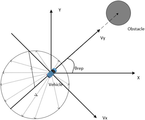
FIGURE 2. Random disturbance process.

2.4 Combination of obstacles

When the distance between two obstacles is too small, it becomes easy for the vehicle to get trapped in a local minimum while navigating between them, and as a result, it may fail to complete the obstacle avoidance action. To address this issue, when multiple obstacles are located too close to each other, they are treated as a significant obstacle for overall obstacle avoidance, as illustrated in Figure 3.

FIGURE 3

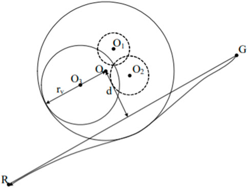
FIGURE 3. Obstacle merging process.

In this scenario, the merged center coordinates (O_x,O_y) and the radius r_v are given in Eqs 17–19:

$O_x=\frac{1}{n}{\displaystyle \sum _{i=0}^n}{O}_{xi}(17)$

$O_y=\frac{1}{n}{\displaystyle \sum _{i=0}^n}{O}_{yi}(18)$

$r_v=\max \left\{‖\left(O_x,O_y\right),\left(O_{xi},O_{yi}\right)‖+r_{vi}\right\},i\in \left[2,n\right](19)$

where O_xi and O_yi are the central coordinate values of each superimposed obstacle; r_vi is the obstacle avoidance radius.

3 Implementation of multi-vehicle formation obstacle avoidance algorithm

3.1 Control methods

The algorithm for multi-vehicle formation obstacle avoidance, based on the improved artificial potential field method, is implemented in MATLAB using the m language. The program follows a modular design, enhancing the system’s scalability. As shown in Figure 4, The main idea of the algorithm is as follows: Firstly, the parameters are initialized, and the initial obstacle avoidance formation is established. The position of the target point is then confirmed to facilitate gravitational calculation. Concurrently, the obstacle environment is assessed to determine whether obstacle merging is required, and boundary information of obstacles is extracted to facilitate repulsion calculation. This is followed by the start of the iterative cycle process to calculate the obstacle avoidance process for the leader and the follower, respectively. The obstacle avoidance process for the leader includes the calculation of the leader’s angle distance, PID control of gravity, calculation of position repulsion and velocity repulsion, calculation of resultant force, and the update of velocity and position. Upon completing the obstacle avoidance process, it is necessary to assess whether the leader has fallen into a local optimum and whether random disturbance is needed to break out of it. Once the leader arrives at the next position, the formation is accordingly adjusted, and the desired position corresponding to the follower can be obtained. On this basis, the obstacle avoidance process for the follower can be completed. The obstacle avoidance process for the followers is essentially like that of the leaders, with the difference lying in the fact that, earlier mentioned leaders take the target point as the expected position and need to complete the repulsion calculation between followers to avoid collisions with each other.

FIGURE 4

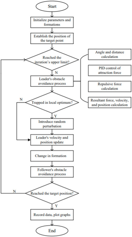
FIGURE 4. Multi-vehicle formation obstacle avoidance process.

3.2 Evaluation function

This paper uses three commonly used evaluation functions: the total iteration times for formation obstacle avoidance, the formation efficiency function, and the standard deviation of iteration times for formation obstacle avoidance. The first two functions assess the performance of the obstacle avoidance algorithm in a specific obstacle environment. At the same time the latter is utilized for evaluating the algorithm’s performance in multi-obstacle environments.

During the formation obstacle avoidance process, the completion of formation obstacle avoidance is determined when the leader and all followers reach their respective desired positions. The recorded time required for this is referred to as the total iteration times of obstacle avoidance. The evaluation function f₁ for the obstacle avoidance algorithm can utilize the total iteration times, denoted as J, for formation obstacle avoidance. A smaller value indicates a higher efficiency in obstacle avoidance.

The formation efficiency function is used to evaluate the damage degree of formation in the process of obstacle avoidance (Zhang et al., 2019). The smaller the formation, the better. Their expressions are as shown in Eqs 20, 21:

$f_2={\displaystyle \sum _{n=1}^N}\left(\left({\displaystyle \sum _{i=1}^I}e\right)/I\right)/N(20)$

$N=J/m(21)$

where i represents the index of each follower, and e represents the deviation between the follower’s actual position and the expected position. J corresponds to the total iteration times of the formation obstacle avoidance process. In order to reduce computational complexity, a predetermined constant iterative interval, denoted as m, is adopted in this study, with a value of 10. Sampling the data at this interval significantly reduces the computational burden. The total number of samples, represented by n, refers to the sequence number of the samples.

The evaluation function f₃ is designed to reflect the energy consumption of the car during obstacle avoidance, including operational and idle power consumption. Specifically, operational energy consumption is associated with the total displacement during the obstacle avoidance process, while idle energy consumption is linked to the total number of iterations in the obstacle avoidance process. The expression for the evaluation function f₃ is as shown in Eq. 22:

$f_3=E_{\text{oc}}+E_{ic}=k_{oc}\cdot J+k_{ic}\cdot s(22)$

where E_oc represents the operational energy consumption, and E_ic represents the idle energy consumption. They are respectively associated with the iteration numbers J and the obstacle avoidance distance s. k_oc and k_ic are their correlation coefficients, with specific values determined based on the relevant environment.

However, when dealing with multiple obstacle environments, the aforementioned efficiency functions alone may not sufficiently capture the adaptability of the formation obstacle avoidance algorithm to the environment. Therefore, the standard deviation of iterative times during the formation obstacle avoidance process is employed as an additional efficiency function to evaluate the effectiveness and rationality of the algorithm (Yanbin et al., 2018). A smaller standard deviation indicates better performance. The expressions for calculating the standard deviation are as shown in Eqs 23, 24:

$f_4=\sqrt{{{\displaystyle \sum _{k=1}^K}\left(J_k-\overline{J}\right)}^2/K}(23)$

$\overline{J}=\left({\displaystyle \sum _{k=1}^K}{J}_k\right)/K(24)$

where k represents the number of simulation experiments, whereas J_k represents the total iteration count for the formation obstacle avoidance in the kth simulation. The aforementioned formulas pertain to calculating the standard deviation and average of the total iteration times. The standard deviation is utilized as an efficiency function to assess the level of discreteness in the obstacle avoidance results. A smaller value indicates a higher adaptability of the obstacle avoidance algorithm to the environment.

4 Simulation experiments and analysis

4.1 Simulation environment and parameter settings

To validate the effectiveness of the multi-vehicle formation obstacle avoidance method proposed in this research, three sets of comparative simulation experiments were conducted using MATLAB programming. The experiments involved comparing the traditional algorithm (APF), the improved algorithm (IAPF), and the proposed algorithm (IPID-APF) under various working conditions. Each algorithm was evaluated within the same obstacle environment.

In all three sets of simulation experiments, the performance parameters were uniformly set, including PID coefficients for leader (K_p, K_i, K_d), PID coefficients for followers (k_p, k_i, k_d), the repulsion coefficients of velocity and position (k_rep, k_v), maximum velocity (V_M), and disturbance velocity (V_R). The details are provided in Table 1:

TABLE 1

TABLE 1. Uniformly setting of performance parameters.

In the first group of experiments, single-vehicle obstacle avoidance was simulated, with three specific obstacle working conditions set as depicted in Figure 5. In the second group, the obstacle avoidance performance of the algorithms was tested in more complex environments by involving multi-vehicle formations and complicating the obstacle layout. Lastly, in the third group, random multiple obstacle environments were utilized, and the efficiency function used to assess the algorithm’s adaptability was the standard deviation of iteration times. This evaluation measured the algorithm’s capacity to handle random environmental conditions.

FIGURE 5

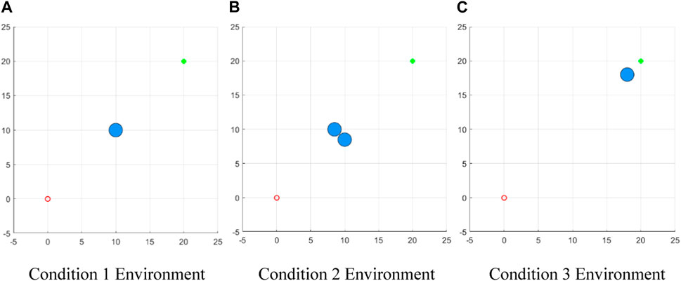
FIGURE 5. Simulation experiment working condition environment. (A) Condition 1 Environment (B) Condition 2 Environment (C) Condition 3 Environment.

4.2 Obstacle avoidance process in setting obstacle environment

In Experiment 1, three working conditions were set. Working condition 1: In this condition, the coordinates of the obstacles were set as (10, 10). This configuration simulates a scenario where the starting point, obstacles, and target points are collinear. Working condition 2: In this condition, the coordinates of the obstacles were set as (10, 8.5) and (8.5, 10). This setup represents a scenario where the vehicle encounters multiple obstacles and may face a local minimum situation. Working condition 3: In this condition, the coordinates of the obstacles were set as (18, 18). This configuration simulates a scenario where obstacles near the target prevent the vehicle from reaching its intended target location. The simulation results of several methods under the above three working conditions are as follows:

As observed in Figure 6, traditional APF method fails to complete obstacle avoidance actions against the three specific obstacles, whereas the improved IAPF method achieves obstacle avoidance but with underwhelming effectiveness, failing to reach the target point within the maximum iteration number of J = 300. Upon introducing PID control, the intelligent surface manages to reach the target under three working conditions with iteration times of J = 143, 181, and 151 respectively. This demonstrates that without altering the gravity and repulsion coefficients of the artificial potential field, the introduction of PID control accelerates the obstacle avoidance process of the vehicle and optimizes the slow speed resulting from the small gravity when approaching the target.

FIGURE 6

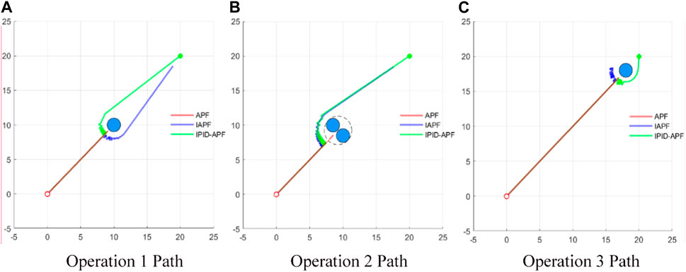
FIGURE 6. Comparison of movement paths under different operating conditions. (A) Operation 1 Path (B) Operation 2 Path (C) Operation 3 Path.

4.3 Obstacle avoidance process in a random obstacle environment

Due to the inadequacy of traditional methods in complex environments, experiment 2 focuses on studying the change in algorithm efficiency before and after the introduction of PID control. The formation consists of five vehicles, with Vehicle 1 serving as the leader and Vehicles 2 to 5 as followers, adopting the common V-shaped formation. This involves adjusting the influence of parameters on the obstacle avoidance efficiency of multi-vehicle formation. Based on setting parameters, PID control is introduced to adjust the remaining parameters, and the algorithm’s performance change is observed. For Experiment 2, three random environments are generated to illustrate the influence of these parameters.

Environment 1:

In Environment 1, the aforementioned results were obtained using two methods. Figure 7 displays the path diagram for vehicle formation obstacle avoidance before and after the implementation of PID control, as well as the diagram indicating the deviation distance between the follower and the leader. Due to the complexity of the obstacle avoidance environment and the presence of random disturbances, the experiment was run 10 times in this particular environment in order to mitigate the impact of randomness.

FIGURE 7

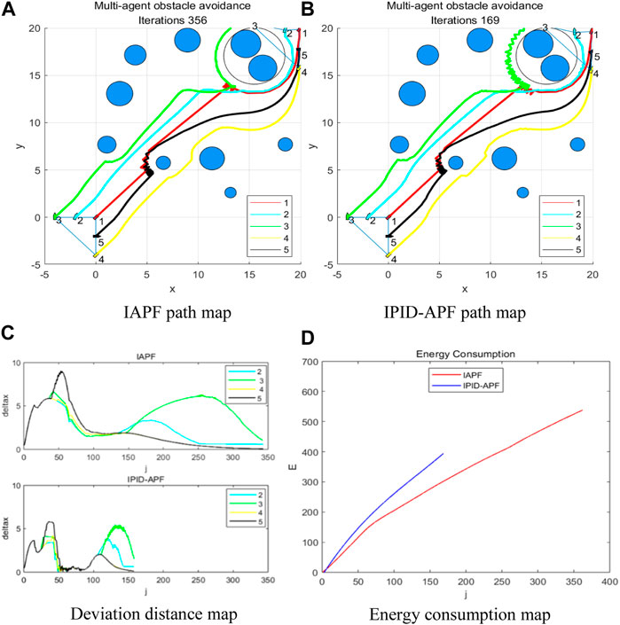
FIGURE 7. Environment 1 maps. (A) IAPF path map (B) IPID-APF path map (C) Deviation distance map (D) Energy consumption map.

After comparing and analyzing the data from the 10 experiments presented in Figure 8, it was observed that the introduction of PID control resulted in a decrease in the average number of iterative times (f₁) for formation obstacle avoidance, reducing it from 361.2 to 209.6. This indicates an acceleration in the rate of formation obstacle avoidance, with an increase of 41.9%. Moreover, the formation efficiency function value (f₂) decreased from an average of 16.3 to 10.0, representing a reduction of 38.7%. This decrease in the function value indicates that the formation remained tighter after the introduction of PID control. Furthermore, the function value (f₃) reflecting energy consumption exhibited a notable decrease, dropping from an average of 562.0 to 337.2, marking a significant 40.0% reduction. This underscores a more energy-efficient obstacle avoidance process. Simultaneously, the analysis of function values across the 10 experiments revealed that random disturbances had a negligible influence. Consequently, conducting multiple experiments in the same environment for future research is deemed unnecessary.

FIGURE 8

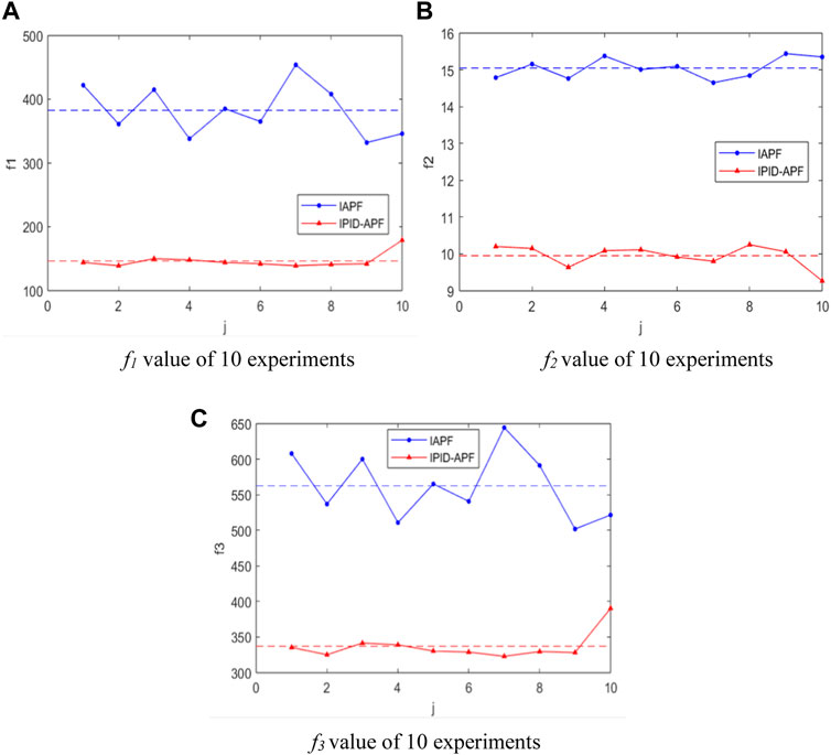
FIGURE 8. Comparison of efficiency functions in environment 1 (10 times average). (A) f₁ value of 10 experiments (B) f₂ value of 10 experiments (C) f₃ value of 10 experiments.

Environment 2:

Comparing the experimental data, it is evident that in comparison to the improved method, the iteration times (f₁) for formation obstacle avoidance decreased from 207 to 79, resulting in a 61.8% increase in the formation obstacle avoidance rate. This acceleration allows the completion of the formation obstacle avoidance task at a faster pace. Additionally, the formation efficiency function value (f₂) decreased from 15.9 to 5.9, marking a 62.9% decrease. This smaller formation damage allows for passing through the obstacle area in a closer formation. Simultaneously, the function value (f3) representing energy consumption decreased significantly by 28.5%, dropping from 351.8 to 251.5.

Based on the obstacle foundation of environment 2, environment 3 increased the number of obstacles from 10 to 15. This is done to further explore the impact of introducing PID control on algorithm performance in a more complex obstacle environment.

Environment 3:

By analyzing the data in Table 4, it is observed that, compared to the proposed method, the improved method shows a decrease in the iteration times (f₁) from 232 to 199, with a change rate of 14.2%. And the formation efficiency function value (f₂) decreases from 16 to 8.4, indicating a reduction of 47.5%. Additionally, the function value (f₃) reflecting energy consumption dropped from 423. 9 to 380.8, marking a significant 10.2% reduction. Due to the increased complexity of the obstacle environment, the simulation results in environment 3, compared to Environment 2, show a less pronounced change in the evaluation function values. However, in environment 3, all evaluation function values (f₁, f₂, f₃) have significantly decreased. This indicates that the proposed method performs well in more complex obstacle environments, improving obstacle avoidance efficiency.

4.4 Obstacle avoidance experiment in 100 times random obstacle environment

To further confirm the adaptability of the multi-vehicle formation obstacle avoidance method in a random obstacle environment, following the analysis of two kinds of random obstacle environments in Experiment 2, 100 experiments were conducted in Experiment 3 to observe the changes in efficiency function values f₁, f₂, and f₃, in order to verify the reliability of this method.

The change curves of function values f₁ and f₂ of the improved algorithm in 100 experiments are compared as follows:

After calculation and statistics, the efficiency function values of 100 experiments $\overline{f_1}$, $\overline{f_2}$, $\overline{f_3}$ and $f_4$ those of 100 experiments can be obtained.

4.5 Discussion

In this paper, three sets of simulation experiments are conducted to thoroughly compare the performance of the traditional algorithm (APF), the improved algorithm (IAPF), and the proposed algorithm (IPID-APF) in various obstacle environments.

Experiment 1 involves three specific obstacle scenarios designed to expose the limitations of the traditional algorithm. As depicted in Figure 6, it is evident that the traditional algorithm fails to complete the obstacle avoidance task. Consequently, for subsequent experiments, the comparison of traditional algorithms is omitted to ensure a more objective and targeted performance evaluation. Experiment 2 encompasses two random obstacle environments, while Experiment 3 entails multiple experiments in complex environments. Most of the algorithms presented in this paper demonstrate superior performance compared to others, as evidenced by the comparison images in Figures 7–11 and the data analysis presented in Tables 2–5. This superior performance is reflected in terms of iteration times, formation maintenance degree, and efficiency function value. These results underscore the significance of incorporating PID control to enhance the algorithm’s performance.

FIGURE 9

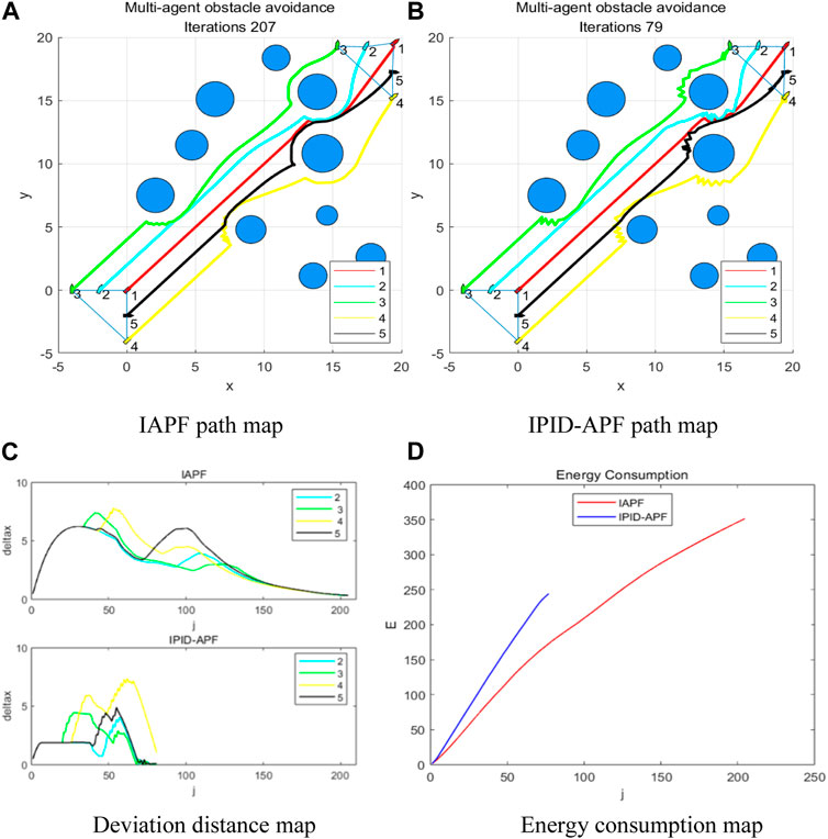
FIGURE 9. Environment 2 maps. (A) IAPF path map (B) IPID-APF path map (C) Deviation distance map (D) Energy consumption map.

FIGURE 10

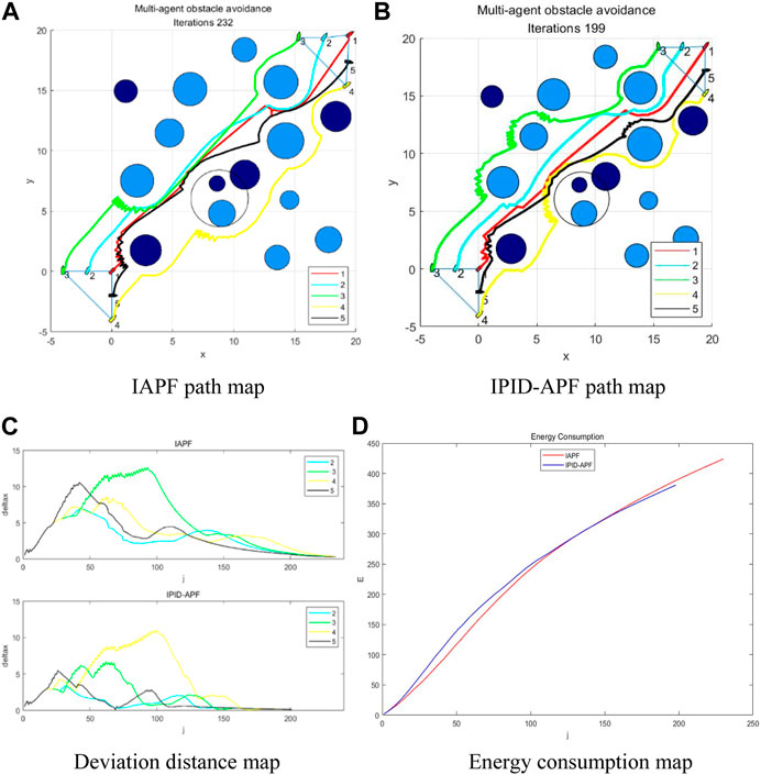
FIGURE 10. Environment 3 maps. (A) IAPF path map (B) IPID-APF path map (C) Deviation distance map (D) Energy consumption map.

FIGURE 11

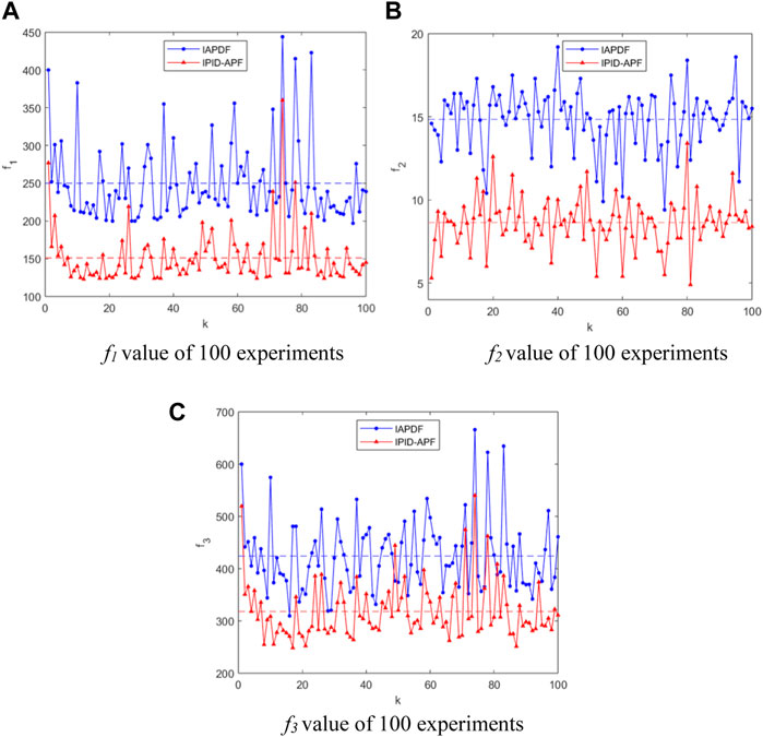
FIGURE 11. Comparison of efficiency functions in random environment (average of 100 times). (A) f₁ value of 10 experiments (B) f₂ value of 10 experiments (C) f₃ value of 10 experiments.

TABLE 2

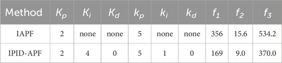
TABLE 2. Setting parameters and corresponding function values in environment 1.

TABLE 3

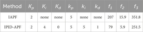
TABLE 3. Setting parameters and corresponding function values ​​in environment 2.

TABLE 4

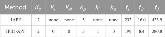
TABLE 4. Setting parameters and corresponding function values in environment 3.

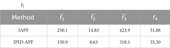
TABLE 5

TABLE 5. $\overline{f_1}$, $\overline{f_2}$, $\overline{f_3}$ and $f_4$ of 100 experiments.

In summary, the proposed algorithm exhibits enhanced formation stability, exceptional obstacle avoidance efficiency, and strong adaptability to environments with random obstacle distribution, as demonstrated by the experimental results. The findings not only showcase the performance advantages of IPID-APF over other algorithms but also offer a reliable and efficient solution to address the obstacle avoidance problem in a random obstacle environment. These insights provide valuable guidance for future research, such as further validation of the effectiveness of IPID-APF in other application scenarios or the finer optimization of PID parameters.

5 Conclusion

This paper proposes a multi-vehicle formation obstacle avoidance algorithm that integrates PID control and an improved artificial potential field method. By incorporating PID control into the potential field function calculation process of the artificial potential field method and introducing an enhanced random disturbance model, issues such as unattainable targets, falling into local optima, and navigating obstacles in a dynamic environment can be effectively addressed. The proposed algorithm is compared with traditional and improved algorithms through simulation experiments conducted in multiple random obstacle scenarios. Four commonly used evaluation functions—total iteration times, formation efficiency function value, energy consumption and standard deviation of iteration times—are employed to assess the algorithm’s performance. The results demonstrate that the efficiency function values of the proposed algorithm are 39.7%, 41.9%, 24.8% and 32.0% higher than those of the other algorithms, respectively. Thus, the proposed algorithm effectively resolves the challenges of multi-vehicle formation control and obstacle avoidance in complex environments.

Data availability statement

The raw data supporting the conclusion of this article will be made available by the authors, without undue reservation.

Author contributions

WY: Writing–original draft, Writing–review and editing. XW: Writing–original draft, Writing–review and editing. GL: Writing–review and editing, Writing–original draft.

Funding

The author(s) declare that no financial support was received for the research, authorship, and/or publication of this article.

Conflict of interest

The authors declare that the research was conducted in the absence of any commercial or financial relationships that could be construed as a potential conflict of interest.

Publisher’s note

All claims expressed in this article are solely those of the authors and do not necessarily represent those of their affiliated organizations, or those of the publisher, the editors and the reviewers. Any product that may be evaluated in this article, or claim that may be made by its manufacturer, is not guaranteed or endorsed by the publisher.

References

Cao, J. F., Ling, Z. H., Gao, C., and Yuan, Y. F. (2014). Obstacle avoidance and formation control for multi-agent based on swarming. J. Syst. Simul. Available at: http://en.cnki.com.cn/Article_en/CJFDTotal-XTFZ201403014.htm (Accessed October 17, 2023). doi:10.16182/j.cnki.joss.2014.03.040

CrossRef Full Text | Google Scholar

Cheng, C., Zhu, D., Sun, B., Chu, Z., Nie, J., and Zhang, S. (2015). “Path planning for autonomous underwater vehicle based on artificial potential field and velocity synthesis,” in 2015 IEEE 28th Canadian Conference on Electrical and Computer Engineering (CCECE), Halifax, NS, Canada (IEEE), 717–721. doi:10.1109/CCECE.2015.7129363

CrossRef Full Text | Google Scholar

Cui, B. X., and Song, J. R. (2018). Obstacle avoidance and dynamic target tracking of robot in unknown environment. J. Shenyang Univ. Technol. 40, 292–298. doi:10.7688/j.issn.1000-1646.2018.03.10

CrossRef Full Text | Google Scholar

Dahiya, A., Aroyo, A. M., Dautenhahn, K., and Smith, S. L. (2023). A survey of multi-agent Human–Robot Interaction systems. Robotics Aut. Syst. 161, 104335. doi:10.1016/j.robot.2022.104335

CrossRef Full Text | Google Scholar

Fan, X., Guo, Y., Liu, H., Wei, B., and Lyu, W. (2020). Improved artificial potential field method applied for AUV path planning. Math. Problems Eng. 2020, 1–21. doi:10.1155/2020/6523158

CrossRef Full Text | Google Scholar

Jia, Q., and Wang, X. (2010). “An improved potential field method for path planning,” in 2010 Chinese Control and Decision Conference, Xuzhou, China (IEEE), 2265–2270. doi:10.1109/CCDC.2010.5498836

CrossRef Full Text | Google Scholar

Khatib, O. (1985). Real-time obstacle avoidance for manipulators and mobile robots. , 2, 500–505. doi:10.1109/robot.1985.1087247

CrossRef Full Text | Google Scholar

Li, G., Yamashita, A., Asama, H., and Tamura, Y. (2012). “An efficient improved artificial potential field based regression search method for robot path planning,” in 2012 IEEE International Conference on Mechatronics and Automation, Chengdu, China (IEEE), 1227–1232. doi:10.1109/ICMA.2012.6283526

CrossRef Full Text | Google Scholar

Matoui, F., Boussaid, B., and Abdelkrim, M. N. (2019). Distributed path planning of a multi-robot system based on the neighborhood artificial potential field approach. SIMULATION 95, 637–657. doi:10.1177/0037549718785440

CrossRef Full Text | Google Scholar

Montiel, O., Sepúlveda, R., and Orozco-Rosas, U. (2015). Optimal path planning generation for mobile robots using parallel evolutionary artificial potential field. J. Intell. Robot. Syst. 79, 237–257. doi:10.1007/s10846-014-0124-8

CrossRef Full Text | Google Scholar

Oh, K.-K., Park, M.-C., and Ahn, H.-S. (2015). A survey of multi-agent formation control. Automatica 53, 424–440. doi:10.1016/j.automatica.2014.10.022

CrossRef Full Text | Google Scholar

Sfeir, J., Saad, M., and Saliah-Hassane, H. (2011). “An improved Artificial Potential Field approach to real-time mobile robot path planning in an unknown environment,” in 2011 IEEE International Symposium on Robotic and Sensors Environments (ROSE), Montreal, QC, Canada (IEEE), 208–213. doi:10.1109/ROSE.2011.6058518

CrossRef Full Text | Google Scholar

Sun, J., Liu, G., Tian, G., and Zhang, J. (2019). Smart obstacle avoidance using a danger index for a dynamic environment. Appl. Sci. 9, 1589. doi:10.3390/app9081589

CrossRef Full Text | Google Scholar

Wang, L., Zhu, D., Pang, W., and Zhang, Y. (2023). A survey of underwater search for multi-target using Multi-AUV: task allocation, path planning, and formation control. Ocean. Eng. 278, 114393. doi:10.1016/j.oceaneng.2023.114393

CrossRef Full Text | Google Scholar

Wu, Z., Dai, J., Jiang, B., and Karimi, H. R. (2023). Robot path planning based on artificial potential field with deterministic annealing. ISA Trans. 138, 74–87. doi:10.1016/j.isatra.2023.02.018

PubMed Abstract | CrossRef Full Text | Google Scholar

Xian-Xia, L., Chao-Ying, L., Xue-Ling, S., and Ying-Kun, Z. (2018). Research on improved artificial potential field approach in local path planning for mobile robot. Comput. Simul. Available at: http://en.cnki.com.cn/Article_en/CJFDTotal-JSJZ201804063.htm (Accessed December 25, 2023). doi:10.3969/j.issn.1006-9348.2018.04.063

CrossRef Full Text | Google Scholar

Yanbin, Z., Pengxue, X. I., Linlin, W., Wenxin, F. a. N., and Mengyun, H. a. N. (2018). Obstacle avoidance method for multi-agent formation based on artificial potential field method. J. Comput. Appl. 38, 3380. doi:10.11772/j.issn.1001-9081.2018051119

CrossRef Full Text | Google Scholar

Yang, X., Yang, W., Zhang, H., Chang, H., Chen, C.-Y., and Zhang, S. (2016). “A new method for robot path planning based artificial potential field,” in 2016 IEEE 11th Conference on Industrial Electronics and Applications (ICIEA), Hefei, China (IEEE), 1294–1299. doi:10.1109/ICIEA.2016.7603784

CrossRef Full Text | Google Scholar

Yang, Y. B., and Wang, C. L. (2013). Obstacle avoidance method for mobile robots based on improved artificial potential field method and its implementation on MATLAB. J. Univ. Shanghai Sci. Technol. Available at: http://www.researchgate.net/publication/312121694_Obstacle_avoidance_method_for_mobile_robots_based_on_improved_artificial_potential_field_method_and_its_implementation_on_MATLAB (Accessed December 25, 2023). doi:10.13255/j.cnki.jusst.2013.05.009

CrossRef Full Text | Google Scholar

Zhang, C. (2018). Path planning for robot based on chaotic artificial potential field method. IOP Conf. Ser. Mater. Sci. Eng. 317, 012056. doi:10.1088/1757-899X/317/1/012056

CrossRef Full Text | Google Scholar

Zhang, X., Su, W., and Chen, L. (2019). “A multi-agent formation control method based on bearing measurement,” in 2019 4th International Conference on Measurement, Information and Control (New York, United States: IEEE). Available at: http://www.xueshufan.com/publication/3016828710 (Accessed December 26, 2023).

CrossRef Full Text | Google Scholar

Zheng, Z., Li, Y., and Wang, Y. (2022). Research and implementation of multi-agent UAV system simulation platform based on JADE. Cham: Springer. doi:10.1007/978-3-030-99200-2_10

CrossRef Full Text | Google Scholar