Optimal scheduling of integrated energy systems with a ladder-type carbon trading mechanism and demand response

Introduction: To achieve the “dual carbon” goal, the integrated energy system (IES) needs to take into account both economic and low-carbon requirements while meeting the growing energy demand.

Methods: Therefore, an optimal scheduling model for low-carbon economic operation is proposed. Firstly, a more accurate carbon emission model is used to consider the actual carbon emission of gas load, to improve the original carbon emission model. A ladder-type carbon trading mechanism is introduced to further constrain the carbon emission of IES. Then, the demand-side response model is proposed, which uses the time-of-use price and mutual substitution of electricity, heat, and gas loads to curtail, time-shift, and substitute the load. Finally, an optimal scheduling model with minimum energy purchase cost, wind and photovoltaic curtailment cost, demand response cost, and carbon emission cost is constructed, which is solved by the GUROBI solver.

Results: Through comparative simulation analysis of 6 cases, the results show that the objective function considers the traditional carbon trading cost to reduce carbon emission by about 19.3% compared with the case without considering. After adopting the ladder-type carbon trading mechanism, the carbon emission of IES can be further limited by about 0.35%, and the appropriate carbon trading base price is explored. In addition, after the demand response, the energy purchase cost, carbon trading cost, and carbon emission of IES are reduced by about 3.4%, 18.5%, and 36.2%, respectively, compared with those before the demand response. The simulation results verify the effectiveness of the proposed model.

1 Introduction

With the continuous acceleration of the global development process and the growing demand for energy, a low-carbon economy and sustainable development have become the consensus of the international community. Therefore, to lead the world development trend, China proposed to achieve “carbon peaking” before 2030 and “carbon neutrality” before 2060 (the “dual carbon” goal). The power industry, as an important part of energy supply, has been increasing its carbon emission every year, so actively controlling its carbon emission will have a profound impact on the promotion of the “dual-carbon” goal (Mallapaty, 2020; Chen et al., 2021a; Li et al., 2021; Chen et al., 2021).

An integrated energy system (IES) is a system that utilizes multiple energy carriers, including electricity, heat, gas, and transmission media, to achieve multi-energy complementarity, intelligent configuration, and optimal scheduling. It achieves efficient use of energy, reduction of energy costs, and reduction of carbon emission (Li et al., 2021), so it has a positive effect on the achievement of the “dual-carbon” goal.

At present, with the economic operation of IES as the research objective, carbon emission during the operation of IES and its significant role in emission reduction cannot be ignored. Under China’s carbon peaking and carbon neutrality goals, carbon emission should be used as part of the objective function of IES or as a consideration to achieve the purpose of reducing carbon emissions (Zhang et al., 2022). Wei et al. (2016) and Lu et al. (2017) added the carbon trading mechanism to the objective function and considered reducing the cost of carbon trading and optimizing the operating cost of IES, which proves that it can effectively suppress the carbon emission of IESs. Carbon emission models were established, and the carbon emission cost was added to the economic operation cost, which realized the emission reduction of the energy supply system and achieved the operation of the low-carbon economy, but their carbon emission models were slightly abbreviated because the carbon emission of the equipment was only linearly related to the power (Li et al., 2019; Tian et al., 2022). Thus, Qu et al. (2018) and Wang et al. (2019) constructed a carbon emission calculation model and introduced a carbon trading mechanism and carbon trading market to precisely construct an optimization model for the low-carbon operation of IESs and realize the low-carbon operation of the economy of IESs. In addition, a ladder-type carbon trading mechanism is introduced to increase carbon trading cost and added to the objective function to further reduce carbon emission of IESs (Qin et al., 2018; Cui et al., 2021). In the current carbon trading market, many researchers only consider the carbon emissions of coal-fired units, gas turbines (GTs), and gas boilers (GBs) while ignoring the carbon emission from the demand-side gas load, which has a huge base of carbon emission and whose impact should be emphasized.

Demand response (DR), as a two-way communication between the supply side and the demand side, is a way for users to participate in the system scheduling. Based on the energy market price and system requirements, users can change their load demand and obtain certain economic compensation (Chen et al., 2019; Chen et al., 2021a). Wei et al. (2022) constructed price-based and substitution-based demand response models that use the price-demand elasticity matrix to describe the impact of energy prices on user demand and realized the inter-substitution between electricity and heat but ignored the substitutability of gas load, which can further reduce the system energy supply cost and carbon emission. A demand-side flexible response model is constructed, which comprehensively considers the mutual substitution of electricity, heat, and gas loads, and the compensation cost of demand response is added as part of the objective function but does not consider the transfer coefficients among electricity, heat, and gas loads and the capacity constraints of substitutable loads, which need to be effectively constrained by the power of energy substitution (Chen et al., 2021).

Consequently, this paper constructs an optimal operation model of the IES based on electricity, heat, and gas loads cogeneration, which comprehensively considers the ladder-type carbon trading mechanism and demand response. Compared with the existing research, the main contributions and innovations of this paper are summarized as follows:

(1) Based on the original carbon emission model, the carbon emission model of the gas load is added, and the ladder-type carbon trading mechanism is introduced to further constrain the carbon emission. The impact of different carbon trading interval lengths and base prices is analyzed on low-carbon operations.

(2) The impact of demand response is analyzed on the operation of a low-carbon economy, and the inter-conversion substitution of the three types of loads is considered to construct a demand response model for three types of loads.

(3) An optimal operation model to minimize the operation cost is established through the simulation analysis, and under the comparison of a variety of cases, the rationality and effectiveness of the model are verified.

The remainder of this paper is organized as follows: Section 2 introduces the IES structure. Section 3 constructs the ladder-type carbon trading mechanism, including the carbon emission initial quota model, the actual carbon emission model, and the ladder-type carbon trading model. Section 4 constructs the electricity–heat–gas demand response model, including price-based and substitution-based demand responses. Section 5 introduces the IES optimal scheduling model, which considers the ladder-type carbon trading mechanism and demand response. Finally, simulation analysis and conclusion are given in Section 6 and Section 7, respectively.

2 IES structure

The IES structure constructed in this paper is shown in Figure 1; the energy supply sources contain a superior power grid, superior gas grid, photovoltaic (PV), and wind turbine (WT). The energy conversion unit contains the gas turbine (GT), gas boiler (GB), heat absorption boiler (HAB), and power-to-gas (P2G). Energy storage units contain electricity, heat, and gas energy storage devices (ES, GS, and HS). The load side contains loads of electricity, heat, and gas, which can jointly participate in the demand response. The total amount of carbon emission from IES includes emissions from the superior grid, gas-consuming devices, and gas load on the demand side, and the P2G device can absorb part of the carbon emission. The carbon emission generated by IES will be measured using the ladder-type carbon trading mechanism.

Figure 1

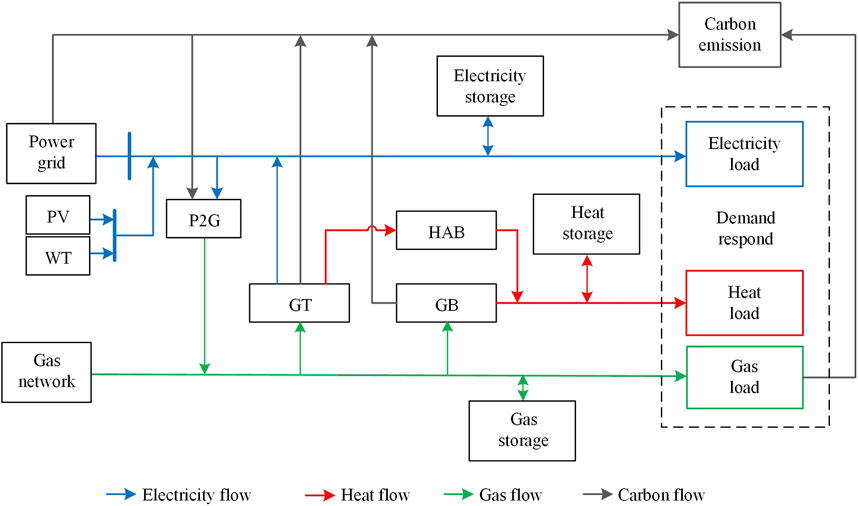
Figure 1. Structure of IES.

3 Ladder-type carbon trading mechanism

Carbon trading is a mechanism to control carbon emissions by establishing legal carbon emission rights and allowing trading. According to the total amount of each emission source, the government or regulatory agencies allocate free emission quotas. If IES emits more carbon than its quota, it needs to buy extra in the carbon trading market; on the contrary, if it emits less than its quota, it can sell the extra emission quota in the market and obtain the corresponding income. The carbon trading mechanism controls carbon emissions through market means, stimulates the enthusiasm of the industry for energy saving and emission reduction, and achieves low-carbon economic operation (Qin et al., 2018). The ladder-type carbon trading mechanism has three main parts: the carbon emission initial quota model, the actual carbon emission model, and the ladder-type carbon trading model.

3.1 The carbon emission initial quota model

In this paper, it is considered that all electricity from the superior power grid is generated by coal-fired units, so the carbon emission sources in the IES include superior coal-fired units, GT, GB, and gas load. The carbon emission quota model is shown as follows:

$\left\{\begin{array}{c}{E}_{\text{IES}}=E_{\text{grid}}+E_{\text{GT}}+E_{\text{GB}}+E_{\text{gload}}\\ E_{\text{grid}}={\chi }_{\mathrm{e}}{\displaystyle \sum _{t=1}^T}{P}_{\text{grid}}\left(t\right)\\ E_{\text{GT}}={\chi }_{\mathrm{h}}{\displaystyle \sum _{t=1}^T}\left({\chi }_{\mathrm{e},\mathrm{h}}{P}_{\text{GT},\mathrm{e}}\left(t\right)+P_{\text{GT},\mathrm{h}}\left(t\right)\right)\\ E_{\text{GB}}={\chi }_{\mathrm{h}}{\displaystyle \sum _{t=1}^T}{P}_{\text{GB},\mathrm{h}}\left(t\right)\\ E_{\text{gload}}={\chi }_{\text{gload}}{\displaystyle \sum _{t=1}^T}{P}_{\mathrm{g},\text{Load}}\left(t\right),\end{array}\right.(1)$

where $E_{\text{IES}}$, $E_{\text{grid}}$, $E_{\text{GT}}$, $E_{\text{GB}}$, and $E_{\text{gload}}$ are the carbon emission quotas of IES, power purchase of the superior power grid, GT, GB, and gas load, respectively; ${\chi }_{\mathrm{e}}$ and ${\chi }_{\mathrm{h}}$ are carbon emission quotas per unit of electric power and heating power generated, respectively; ${\chi }_{\text{gload}}$ is the carbon emission quota per unit of the gas load consumed; ${\chi }_{\mathrm{e},\mathrm{h}}$ is the electric-to-heat coefficient; $P_{\text{grid}}\left(t\right)$ is the electricity quantity purchased from the superior power grid in the time period t; $P_{\text{GT},\mathrm{e}}\left(t\right)$ and $P_{\text{GT},\mathrm{h}}\left(t\right)$ are, respectively, the electric power and heating power of GT in the time period t; $P_{\text{GB},\mathrm{h}}\left(t\right)$ is the heating power of GB in the time period t; $P_{\mathrm{g},\text{Load}}\left(t\right)$ is the gas load consumed in the time period t; $T$ is the scheduling period.

3.2 The actual carbon emission model

The P2G device can absorb part of the carbon emission by consuming electricity. The gas load consumed on the demand side also generates carbon emissions and cannot be ignored, so the actual carbon emission model is improved to consider the carbon emission from the gas load as well (Qin et al., 2018; Chen et al., 2021a; Chen et al., 2021c). The actual carbon emission model is shown as follows:

$\left\{\begin{array}{c}{E}_{\text{lES},\mathrm{a}}=E_{\text{grid},\mathrm{a}}+E_{\text{gtgb},\mathrm{a}}+E_{\text{gload},\mathrm{a}}-E_{\mathrm{P}2\mathrm{G},\mathrm{a}}\\ E_{\text{grid}}={\displaystyle \sum _{i=1}^T}\left[a_1+b_1{P}_{\text{grid}}\left(t\right)+c_1{P}_{\text{grid}}^2\left(t\right)\right]\\ E_{\text{gtgb},\mathrm{a}}={\displaystyle \sum _{i=1}^T}\left[a_2+b_2{P}_{\text{gtgb}}\left(t\right)+c_2{P}_{\text{gtgb}}^2\left(t\right)\right]\\ P_{\text{gtgb}}\left(t\right)=P_{\text{GT},\mathrm{e}}\left(t\right)+P_{\text{GT},\mathrm{h}}\left(t\right)+P_{\text{GB},\mathrm{h}}\left(t\right)\\ E_{\text{gload},\mathrm{a}}={\displaystyle \sum _{i=1}^T}\xi P_{\mathrm{g},\text{Load}}\left(t\right)\\ E_{\mathrm{P}2\mathrm{G},\mathrm{a}}={\displaystyle \sum _{t=1}^T}\varpi P_{\mathrm{P}2\mathrm{G},\mathrm{g}}\left(t\right),\end{array}\right.(2)$

where $E_{\text{lES},\mathrm{a}}$ is the actual total carbon emission of IES; $E_{\text{grid},\mathrm{a}}$ is the actual carbon emission from the coal-fired unit purchasing power from the superior power grid; $E_{\text{gtgb},\mathrm{a}}$ is the actual total carbon emission of GT and GB; $E_{\text{gload},\mathrm{a}}$ is the actual total carbon emission of gas load; $E_{\mathrm{P}2\mathrm{G},\mathrm{a}}$ is the carbon emission absorbed by the P2G device; $P_{\text{gtgb}}\left(t\right)$ is the total generating power of GT and GB in the time period t; $a_1$, $b_1$, and $c_1$ are the carbon emission calculation coefficients of the coal-fired unit; $a_2$, $b_2$, and $c_2$ are the carbon emission coefficients of the natural gas energy supply; $\xi$ is the equivalent carbon emission coefficient per unit gas load (Zhao et al., 2021); $\varpi$ is the carbon emission coefficient absorbed by the P2G device; $P_{\mathrm{P}2\mathrm{G},\mathrm{g}}\left(t\right)$ is the power of natural gas emitted by the P2G device in the time period t.

3.3 The ladder-type carbon trading model

The carbon emission of the IES participating in carbon trading is represented as follows:

$E_{\text{IES},\mathrm{t}}=E_{\text{IES},\mathrm{a}}-E_{\text{IES}}.(3)$

In the traditional carbon trading mechanism, the base price of carbon trading is fixed, while the ladder-type carbon trading mechanism divides carbon emissions into several purchase intervals. As the carbon trading account of the IES continues to increase, the carbon trading cost will also increase. The ladder-type carbon trading model is as follows:

$C_{{\text{CO}}_2}=\left\{\begin{array}{c}\lambda E_{\text{lES},\mathrm{t}},E_{\text{lES},\mathrm{t}}\le l\\ \lambda \left(1+\alpha \right)\left(E_{\text{lES},\mathrm{t}}-l\right)+\lambda l,l<E_{\text{lES},\mathrm{t}}\le 2l\\ \lambda \left(1+2\alpha \right)\left(E_{\text{lES},\mathrm{t}}-2l\right)+\left(2+\alpha \right)\lambda l,2l<E_{\text{lES},\mathrm{t}}\le 3l\\ \lambda \left(1+3\alpha \right)\left(E_{\text{lES},\mathrm{t}}-3l\right)+\left(3+3\alpha \right)\lambda l,3l<E_{\text{lES},\mathrm{t}}\le 4l\\ \lambda \left(1+4\alpha \right)\left(E_{\text{lES},\mathrm{t}}-4l\right)+\left(4+6\alpha \right)\lambda l,4l<E_{\text{lES},\mathrm{t}}\end{array}\right.(4)$

where $C_{{\text{CO}}_2}$ is the carbon trading cost of IES; $\lambda$ is the base price of carbon trading; $\alpha$ is the increasing extent of price; $l$ is the length of the carbon emission interval.

4 The electricity–heat–gas demand response model

In the demand response of electricity load, the electricity load can be adjusted according to the characteristics of time-of-use electricity price, and the electricity price power elasticity coefficient is commonly used to describe the changing relationship between the price and load. Therefore, for the heat and gas loads, the load can also be adjusted, and the demand response can be conducted according to the time-of-use heat price and gas price to further realize the economy of IESs.

In addition, it is also necessary to pay attention to the mutual substitution effect of electricity, heat, and gas loads. Through the energy conversion devices inside IES, energy coupling is realized, and it participates in the energy response in the form of multi-energy complementarity. Therefore, loads can participate in demand response not only in their original form but also by substituting other energy sources.

Accordingly, the loads are divided into curtailable, time-shifted, and substitutable loads, and this paper divides the demand response into two segments: first, based on time-of-use prices, electric, heat, and gas loads are subjected to price-based demand response to time-shift and curtail loads; second, utilizing the mutual substitutability of electricity, heat, and gas loads for substitution-based demand response, substitutable energy sources can achieve low-carbon economic operation of IESs.

4.1 Price-based demand response

To guide users to carry out reasonable and standardized energy consumption behavior, the time-of-use electricity price is proposed to curtail and time-shift the electric load curve and achieve the effect of peak-shaving and valley-filling. For heat and gas loads, the loads can also be adjusted according to the peak–flat–valley price to achieve economic operation. The electricity price–quantity elasticity matrix method is a commonly used price-based demand response modeling method, and the electricity price–quantity elasticity coefficient indicates the relationship between the customer’s electricity consumption behavior and changes in electricity price (Thimmapuram and Kim, 2013; Kong et al., 2015). Its expression is represented as follows:

$e_{\mathrm{i},\mathrm{j}}=\frac{\Delta d_{\mathrm{i}}/d_{\mathrm{i}}^0}{\Delta {\rho }_{\mathrm{j}}/{\rho }_{\mathrm{j}}^0},(5)$

where $e_{\mathrm{i},\mathrm{j}}$ is the elasticity coefficient of load in time period i with regard to electricity price in time period j; $d_{\mathrm{i}}^0$ is the initial load in time period i; $\Delta d_{\mathrm{i}}$ is the variation in load caused by price change in time period i; ${\rho }_{\mathrm{j}}^0$ is the initial electricity price in time period j; $\Delta {\rho }_{\mathrm{j}}$ is the variation of price in time period j.

Regardless of electricity load or heat and gas loads, for their respective time-of-use prices, the elasticity coefficient of a user’s load in time period i with regard to the price in time period j can be defined as follows:

$E_{\mathrm{L}}\left(i,j\right)=\frac{{\mathrm{d}}_{\mathrm{L}}\left(i\right)-d_{\mathrm{L},0}\left(i\right)}{\rho \left(j\right)-{\rho }_0\left(j\right)}\frac{{\rho }_0\left(j\right)}{d_{\mathrm{L},0}\left(i\right)}.(6)$

When $i=j$, it is $E_{\mathrm{L}}\left(i\right)$, referred to as the self-elasticity coefficient, which indicates the variation in load in time period i relative to the variation in price in the same time period; when $i\ne j$, referred to as the cross-elasticity coefficient, it indicates the variation in load in time period i relative to the variation in price in time period j. In general, the load in a certain time period is inversely proportional to the price in the same time period and directly proportional to the price in other time periods, so $E_{\mathrm{L}}\left(i\right)\le 0$ and $E_{\mathrm{L}}\left(i,j\right)\ge 0$.

The variation in load in time period i with regard to the time-of-use price can be expressed as follows:

$d_{\mathrm{L}}\left(j\right)=d_{\mathrm{L},0}\left(j\right)+{\displaystyle \sum _{j=1}^{24}}\left\{E_{\mathrm{L}}\left(i,j\right)\frac{d_{\mathrm{L},0}\left(j\right)}{{\rho }_0\left(j\right)}\left[\rho \left(j\right)-{\rho }_0\left(j\right)\right]\right\}.(7)$

Let ${\lambda }_{\mathrm{L}}\left(i\right)$ indicate that, after the implementation of time-of-use price, the rate of variation in load in time period i is expressed as follows:

${\lambda }_{\mathrm{L}}\left(i\right)=\frac{d_{\mathrm{L}}\left(i\right)-d_{\mathrm{L},0}\left(i\right)}{d_{\mathrm{L},0}\left(0\right)}={\displaystyle \sum _{j=1}^{24}}\left\{E_{\mathrm{L}}\left(i,j\right)\frac{\left[\rho \left(i\right)-{\rho }_0\left(j\right)\right]}{{\rho }_0\left(j\right)}\right\}.(8)$

If $k\left(i\right)=\frac{\rho \left(i\right)-{\rho }_0\left(i\right)}{{\rho }_0\left(i\right)}$ is referred to as the price-float ratio, which describes the extent of price fluctuation caused by time-of-use price, and considering the time-shifted and curtailed part of the load, then ${\lambda }_{\mathrm{L}}\left(i\right)$ can be expressed as follows:

${\lambda }_{\mathrm{L}}\left(i\right)={\displaystyle \sum _{j=1,j\ne i}^{24}}{E}_{\mathrm{L}}\left(i,j\right)k\left(j\right)+E_{\mathrm{L}}\left(i\right)k\left(i\right),(9)$

where the first term is the load time-shift from time period i to time period j; the second term is the load curtailed in time period i.

From this, the rate of variation in load among the peak, flat, and valley time periods can be obtained as follows:

$\left\{\begin{array}{cc}{\lambda }_{\text{pp}}=k_{\mathrm{p}}{E}_{\mathrm{L}}\left(i\right)& \forall i\in T_{\mathrm{p}}\\ {\lambda }_{\text{ff}}=k_{\mathrm{f}}{E}_{\mathrm{L}}\left(i\right)& \forall i\in T_{\mathrm{f}}\\ {\lambda }_{\text{vv}}=k_{\mathrm{v}}{E}_{\mathrm{L}}\left(i\right)& \forall i\in T_{\mathrm{v}}\\ {\lambda }_{\text{pf}}=\left(k_{\mathrm{p}}-k_{\mathrm{f}}\right)E_{\mathrm{L}}\left(i,j\right)& \forall i\in T_{\mathrm{p}},j\in T_{\mathrm{f}}\\ {\lambda }_{\text{pv}}=\left(k_{\mathrm{p}}-k_{\mathrm{v}}\right)E_{\mathrm{L}}\left(i,j\right)& \forall i\in T_{\mathrm{p}},j\in T_{\mathrm{v}}\\ {\lambda }_{\text{fv}}=\left(k_{\mathrm{f}}-k_{\mathrm{v}}\right)E_{\mathrm{L}}\left(i,j\right)& \forall i\in T_{\mathrm{f}},j\in T_{\mathrm{v}},\end{array}\right.(10)$

where $T_{\mathrm{p}}$, $T_{\mathrm{f}}$, and $T_{\mathrm{v}}$ are the peak, flat, and valley time periods divided according to the time-of-use price, respectively; ${\lambda }_{\text{pf}}$, ${\lambda }_{\text{pv}}$, and ${\lambda }_{\text{fv}}$ indicate the time-shift of load, respectively; ${\lambda }_{\text{pp}}$, ${\lambda }_{\text{ff}}$, and ${\lambda }_{\text{vv}}$ indicate the peak-shaving and valley-filling effects of the load in this time period; this paper argues that the flat periods’ price after the implementation of time-of-use price is higher than before so that in peak periods, $k_{\mathrm{p}}>0$; in flat periods, $k_{\mathrm{f}}>0$; and in valley periods, $k_{\mathrm{v}}<0$; therefore, ${\lambda }_{\text{pp}}$ and ${\lambda }_{\text{ff}}$ are negative numbers; ${\lambda }_{\text{vv}}$ is a positive number; and ${\lambda }_{\text{pf}}$, ${\lambda }_{\text{pv}}$, and ${\lambda }_{\text{fv}}$ are positive numbers. The value of $E_{\mathrm{L}}\left(i,j\right)$ needs to be obtained through social surveys such as price fluctuations and user load conditions, and the methodology will not be described in this paper; for the specific values, refer to Zhang et al. (2021).

In summary, the demand response model after the implementation of time-of-use price can be represented as follows:

${\mathit{d}}^{\prime }=\mathit{d}+\mathit{\lambda }\times \mathit{d}(11)$

and

$\left.\mathit{\lambda }=\left[\begin{array}{ccc}{\lambda }_{\text{pp}}& -{\lambda }_{\text{pf}}& -{\lambda }_{\text{pv}}\\ {\lambda }_{\text{pf}}& {\lambda }_{\text{ff}}& -{\lambda }_{\text{fv}}\\ {\lambda }_{\text{pv}}& {\lambda }_{\text{fv}}& {\lambda }_{\text{vv}}\end{array}\right.\right],\mathit{d}=\left[\begin{array}{c}{d}_{\mathrm{p}}\\ d_{\mathrm{f}}\\ d_{\mathrm{v}}\end{array}\right],(12)$

where $d_{\mathrm{p}}$, $d_{\mathrm{f}}$, and $d_{\mathrm{v}}$ are the loads in the peak, flat, and valley periods before demand response, respectively; ${\mathit{d}}^{\prime }$ is the quantity of loads after participating in the demand response.

Based on the above demand response method, according to the time-of-use electricity price, heat price, and gas price, this paper makes a preliminary price-based demand response to the three types of loads to time-shift and curtail loads.

4.2 Substitution-based demand response

Users have flexibility in their demand for various types of loads and can choose different energy demands to meet their needs in the same time period to achieve energy saving and emission reduction through an economic lifestyle. For example, ① regarding electricity demand, part of the electricity is used to meet hot water or warming demand, and users can choose to use the heating power provided by the IES or use a gas water heater; ② regarding heating demand, part of the heating power is used for warming or hot water demand, and users can choose to use the electric air conditioner or gas water heater; ③ regarding gas demand, part of the natural gas is used for warming or cooking demand, and users can choose to use an induction cooker and use the heating power provided by the IES for warming. Substitution-based demand response does not change the user’s demand for load and affect the users, and it also compensates the users to stimulate the behavior; therefore, the substitution-based demand response model can be expressed as follows:

$\left\{\begin{array}{l}{P}_{\text{ptg}}\left(t\right)\cdot P_{\text{gtp}}\left(t\right)=0\\ P_{\text{pth}}\left(t\right)\cdot P_{\text{htp}}\left(t\right)=0\\ P_{\text{gth}}\left(t\right)\cdot P_{\text{htg}}\left(t\right)=0\\ 0\le P_{\text{ptg}}\left(t\right)+P_{\text{pth}}\left(t\right)\le {\omega }_{\mathrm{e}}{P}_{\mathrm{e},\text{load}}^{\prime }\left(t\right)\\ 0\le P_{\text{htg}}\left(t\right)+P_{\text{htp}}\left(t\right)\le {\omega }_{\mathrm{h}}{P}_{\mathrm{h},\text{load}}^{\prime }\left(t\right)\\ 0\le P_{\text{gtp}}\left(t\right)+P_{\text{gth}}\left(t\right)\le {\omega }_{\mathrm{g}}{P}_{\mathrm{g},\text{load}}^{\prime }\left(t\right)\\ 0\le P_{\text{htp}}\left(t\right)/{\eta }_{\text{pth}}+{\eta }_{\text{gth}}{P}_{\text{gtp}}\left(t\right)/{\eta }_{\text{pth}}\le {\omega }_{\text{te}}{P}_{\mathrm{e},\text{load}}^{\prime }\left(t\right)\\ 0\le {\eta }_{\text{pth}}{P}_{\text{pth}}\left(t\right)+{\eta }_{\text{gth}}{P}_{\text{gth}}\left(t\right)\le {\omega }_{\text{th}}{P}_{\mathrm{h},\text{load}}^{\prime }\left(t\right)\\ 0\le P_{\text{htg}}\left(t\right)/{\eta }_{\text{gth}}+{\eta }_{\text{pth}}{P}_{\text{ptg}}\left(t\right)/{\eta }_{\text{gth}}\le {\omega }_{\text{tg}}{P}_{\mathrm{g},\text{load}}^{\prime }\left(t\right),\end{array}\right.(13)$

where $P_{\text{ptg}}\left(t\right)$ and $P_{\text{pth}}\left(t\right)$ are the electric power that is substituted into gas power and heating power in time period t, respectively; $P_{\text{htp}}\left(t\right)$ and $P_{\text{htg}}\left(t\right)$ are the heating power that is substituted into electric power and gas power in time period t, respectively; $P_{\text{gtp}}\left(t\right)$ and $P_{\text{gth}}\left(t\right)$ are the gas power that is substituted into electric power and heating power in time period t, respectively; ${\omega }_{\mathrm{e}}$, ${\omega }_{\mathrm{h}}$, and ${\omega }_{\mathrm{g}}$ are the ratios of substitutable loads that can be transferred out from electricity, heat, and gas loads, respectively; ${\omega }_{\text{te}}$, ${\omega }_{\text{th}}$, and ${\omega }_{\text{tg}}$ are the ratios of substitutable loads that can be transferred in the electricity, heat, and gas loads, respectively; ${\eta }_{\text{pth}}$ is the electric-to-heat coefficient; ${\eta }_{\text{gth}}$ is the gas-to-heat coefficient; $P_{\mathrm{e},\text{load}}^{\prime }\left(t\right)$, $P_{\mathrm{h},\text{load}}^{\prime }\left(t\right)$, and $P_{\mathrm{g},\text{load}}^{\prime }\left(t\right)$ are the electricity, heat, and gas loads after price-based demand response in time period t, respectively.

Eventually, the electricity, heat, and gas loads after price-based and substitution-based demand response can be obtained, which are as shown in the following:

$\left\{\begin{array}{l}{P}_{\mathrm{e},\text{load}}\left(t\right)=P_{\mathrm{e},\text{load}}^{\prime }\left(t\right)-P_{\text{ptg}}\left(t\right)-P_{\text{pth}}\left(t\right)+P_{\text{htp}}\left(t\right)/{\eta }_{\text{pth}}+{\eta }_{\text{gth}}{P}_{\text{gtp}}\left(t\right)/{\eta }_{\text{pth}}\\ P_{\mathrm{h},\text{load}}\left(t\right)=P_{\mathrm{h},\text{load}}^{\prime }\left(t\right)-P_{\text{htg}}\left(t\right)-P_{\text{htp}}\left(t\right)+{\eta }_{\text{pth}}{P}_{\text{pth}}\left(t\right)+{\eta }_{\text{gth}}{P}_{\text{gth}}\left(t\right)\\ P_{\mathrm{g},\text{load}}\left(t\right)=P_{\mathrm{g},\text{load}}^{\prime }\left(t\right)-P_{\text{gtp}}\left(t\right)-P_{\text{gth}}\left(t\right)+P_{\text{htg}}\left(t\right)/{\eta }_{\text{gth}}+{\eta }_{\text{pth}}{P}_{\text{ptg}}\left(t\right)/{\eta }_{\text{gth}}.\end{array}\right.(14)$

5 Optimal scheduling model of IES with the ladder-type carbon trading mechanism and demand response

5.1 Objective function

The IES constructed in this paper considers the costs of carbon trading and demand response and takes the lowest comprehensive cost as the objective function, including the energy purchase cost $C_{\text{Buy}}$, wind and photovoltaic curtailment cost $C_{\text{DG},\text{cut}}$, demand response cost $C_{\text{DR}}$, and carbon trading cost $C_{\mathrm{C}{\mathrm{O}}_2}$, which are as shown in the following:

$C=C_{\text{Buy}}+C_{\text{DG},\text{cut}}+C_{\text{DR}}+C_{\mathrm{C}{\mathrm{O}}_2}.(15)$

(1) Energy purchase cost $C_{\text{Buy}}:$

$C_{\text{buy}}={\displaystyle \sum _{t=1}^T}{\alpha }_{\mathrm{t}}{P}_{\text{grid}}\left(t\right)+{\displaystyle \sum _{t=1}^T}{\beta }_{\mathrm{t}}{P}_{\mathrm{g},\text{buy}}\left(t\right),(16)$

where $P_{\mathrm{g},\text{buy}}\left(t\right)$ is the gas amount purchased by the IES in time period t; ${\alpha }_{\mathrm{t}}$ and ${\beta }_{\mathrm{t}}$ are the prices of electricity and natural gas in time period t, respectively.

(2)Wind and photovoltaic curtailment cost $C_{\text{DG},\text{cut}}:$

$\left\{\begin{array}{l}{C}_{\text{DG},\text{cut}}={\delta }_{\text{DG}}{\displaystyle \sum _{t=1}^T}{P}_{\text{DG},\text{cut}}\left(t\right)\\ P_{\text{DG},\text{cut}}\left(t\right)=P_{\text{PV}}^{\max }\left(t\right)+P_{\text{WT}}^{\max }\left(t\right)-P_{\text{PV}}\left(t\right)-P_{\text{WT}}\left(t\right),\end{array}\right.(17)$

where ${\delta }_{\text{DG}}$ is the penalty cost per unit of wind and photovoltaic curtailment power; $P_{\text{DG},\text{cut}}\left(t\right)$ is the electric power of wind and photovoltaic curtailment in time period t; $P_{\text{PV}}^{\max }\left(t\right)$ and $P_{\text{WT}}^{\max }\left(t\right)$ are the upper limits of photovoltaic and wind power generated in time period t, respectively; $P_{\text{PV}}\left(t\right)$ and $P_{\text{WT}}\left(t\right)$ are the power generated by photovoltaic and wind power in time period t, respectively.

(3)Demand response cost $C_{\text{DR}}:$

$\left.C_{\text{DR}}={\delta }_{\text{DR}}{\displaystyle \sum _{t=1}^T}\left[P_{\text{ptg}}\right.\left(t\right)+P_{\text{pth}}\left(t\right)+P_{\text{htg}}\left(t\right)+P_{\text{htp}}\left(t\right)+P_{\text{gtp}}\left(t\right)+P_{\text{gth}}\left(t\right)\right],(18)$

where ${\delta }_{\text{DR}}$ is the unit compensation coefficient for participation in the substitution-based demand response.

(4)Carbon trading cost $C_{\mathrm{C}{\mathrm{O}}_2}:$

The calculation of carbon trading cost is shown in Equation 4:

5.2 Constraints

5.2.1 Wind and photovoltaic power constraints

$\left\{\begin{array}{l}0\le P_{\text{PV}}\left(t\right)\le P_{\text{PV}}^{\max }\left(t\right)\\ 0\le P_{\text{WT}}\left(t\right)\le P_{\text{WT}}^{\max }\left(t\right).\end{array}\right.(19)$

5.2.2 Gas turbine constraints

$\left\{\begin{array}{l}{P}_{\text{GT},\mathrm{e}}\left(t\right)={\eta }_{\text{GT}}^{\mathrm{e}}{P}_{\mathrm{g},\text{GT}}\left(t\right)\\ P_{\text{GT},\mathrm{e}}^{\min }\le P_{\text{GT},\mathrm{e}}\left(t\right)\le P_{\text{GT},\mathrm{e}}^{\max }\\ \Delta P_{\text{GT},\mathrm{e}}^{\min }\le P_{\text{GT},\mathrm{e}}\left(t+1\right)-P_{\text{GT},\mathrm{e}}\left(t\right)\le \Delta P_{\text{GT},\mathrm{e}}^{\max },\end{array}\right.(20)$

where ${\eta }_{\text{GT}}^{\mathrm{e}}$ is the gas-to-electric coefficient of GT; $P_{\mathrm{g},\text{GT}}\left(t\right)$ is the gas power input to the GT in time period t; $P_{\text{GT},\mathrm{e}}^{\max }$ and $P_{\text{GT},\mathrm{e}}^{\min }$ are the upper and lower limits of GT output electric power, respectively; $\Delta P_{\text{GT},\mathrm{e}}^{\max }$ and $\Delta P_{\text{GT},\mathrm{e}}^{\min }$ are ramp upper and lower limits of GT output electric power, respectively.

5.2.3 Heat absorption boiler constraints

$\left\{\begin{array}{l}{P}_{\text{HA},\mathrm{h}}\left(t\right)={\eta }_{\text{HA}}\times P_{{\text{HA}}_{-}\text{in},\mathrm{h}}\left(t\right)\\ 0\le P_{{\text{HA}}_{-}\text{in},\mathrm{h}}\left(t\right)\le {\eta }_{\text{GT}}^{\mathrm{h}}\times P_{\mathrm{g},\text{GT}}\left(t\right)\\ P_{\text{HA},\mathrm{h}}^{\min }\le P_{\text{HA},\mathrm{h}}\left(t\right)\le P_{\text{HA},\mathrm{h}}^{\max }\\ \Delta P_{\text{HA},\mathrm{h}}^{\min }\le P_{\text{HA},\mathrm{h}}\left(t+1\right)-P_{\text{HA},\mathrm{h}}\left(t\right)\le \Delta P_{\text{HA},\mathrm{h}}^{\max },\end{array}\right.(21)$

where ${\eta }_{\text{HA}}$ is the absorption efficiency of HAB; ${\eta }_{\text{GT}}^{\mathrm{h}}$ is the gas-to-heat coefficient of GT; $P_{\text{HA},\mathrm{h}}\left(t\right)$ is the output heating power of HAB in time period t; $P_{{\text{HA}}_{-}\text{in},\mathrm{h}}\left(t\right)$ is the heating power absorbed by HAB in time period t; $P_{\text{HA},\mathrm{h}}^{\max }$ and $P_{\text{HA},\mathrm{h}}^{\min }$ are the upper and lower limits of HAB output heating power, respectively; $\Delta P_{\text{HA},\mathrm{h}}^{\max }$ and $\Delta P_{\text{HA},\mathrm{h}}^{\min }$ are ramp upper and lower limits of HAB output heating power, respectively.

5.2.4 Gas boiler constraints

$\left\{\begin{array}{c}{P}_{\text{GB},\mathrm{h}}\left(t\right)={\eta }_{\text{GB}}{P}_{\mathrm{g},\text{GB}}\left(t\right)\\ P_{\text{GB},\mathrm{h}}^{\min }\le P_{\text{GB},\mathrm{h}}\left(t\right)\le P_{\text{GB},\mathrm{h}}^{\max }\\ \Delta P_{\text{GB},\mathrm{h}}^{\min }\le P_{\text{GB},\mathrm{h}}\left(t+1\right)-P_{\text{GB},\mathrm{h}}\left(t\right)\le \Delta P_{\text{GB},\mathrm{h}}^{\max },\end{array}\right.(22)$

where ${\eta }_{\text{GB}}$ is the gas-to-heat coefficient of GB; $P_{\mathrm{g},\text{GB}}\left(t\right)$ is the gas power input to the GB in time period t; $P_{\text{GB},\mathrm{h}}^{\max }$ and $P_{\text{GB},\mathrm{h}}^{\min }$ are the upper and lower limits of GB output heating power, respectively; $\Delta P_{\text{GB},\mathrm{h}}^{\max }$ and $\Delta P_{\text{GB},\mathrm{h}}^{\min }$ are ramp upper and lower limits of GB output heating power, respectively.

5.2.5 P2G device constraints

$\left\{\begin{array}{l}{P}_{\mathrm{P}2\mathrm{G},\mathrm{g}}\left(t\right)={\eta }_{\mathrm{P}2\mathrm{G}}{P}_{\mathrm{e},\mathrm{P}2\mathrm{G}}\left(t\right)\\ P_{\mathrm{P}2\mathrm{G},\mathrm{g}}^{\min }\le P_{\mathrm{P}2\mathrm{G},\mathrm{g}}\left(t\right)\le P_{\mathrm{P}2\mathrm{G},\mathrm{g}}^{\max }\\ \Delta P_{\mathrm{P}2\mathrm{G},\mathrm{g}}^{\min }\le P_{\mathrm{P}2\mathrm{G},\mathrm{g}}\left(t+1\right)-P_{\mathrm{P}2\mathrm{G},\mathrm{g}}\left(t\right)\le \Delta P_{\mathrm{P}2\mathrm{G},\mathrm{g}}^{\max },\end{array}\right.(23)$

where ${\eta }_{\mathrm{P}2\mathrm{G}}$ is the conversion coefficient of the P2G device; $P_{\mathrm{e},\mathrm{P}2\mathrm{G}}\left(t\right)$ is the electric power input to the P2G in time period t; $P_{\mathrm{P}2\mathrm{G},\mathrm{g}}^{\max }$ and $P_{\mathrm{P}2\mathrm{G},\mathrm{g}}^{\min }$ are the upper and lower limits of P2G output gas power, respectively; $\Delta P_{\mathrm{P}2\mathrm{G},\mathrm{g}}^{\max }$ and $\Delta P_{\mathrm{P}2\mathrm{G},\mathrm{g}}^{\min }$ are ramp upper and lower limits of P2G output gas power, respectively.

5.2.6 Energy storage device constraints

This paper constructs an IES containing three types of energy storage devices, namely, electricity, heat, and gas, which further improves the flexibility of operation, and the energy storage devices have similar models, so they are modeled uniformly.

$\left\{\begin{array}{l}-u_{\text{ES},\mathrm{n}}\left(t\right)P_{\text{ES},\mathrm{n}}^{\max }\le P_{\text{ES},\mathrm{n}}^{\text{in}}\left(t\right)\le 0\\ 0\le P_{\text{ES},\mathrm{n}}^{\text{out}}\left(t\right)\le \left[1-u_{\text{ES},\mathrm{n}}\left(t\right)\right]P_{\text{ES},\mathrm{n}}^{\max }\\ P_{\text{ES},\mathrm{n}}\left(t\right)=P_{\text{ES},\mathrm{n}}^{\text{out}}\left(t\right)/{\eta }_{\text{ES},\mathrm{n}}^{\text{out}}+P_{\text{ES},\mathrm{n}}^{\text{in}}\left(t\right){\eta }_{\mathrm{{\rm E}}\mathrm{S},\mathrm{n}}^{\text{in}}\\ S_{\mathrm{n}}\left(t\right)=\left(1-{\sigma }_{\text{ES},\mathrm{n}}\right)S_{\mathrm{n}}\left(t-1\right)-P_{\text{ES},\mathrm{n}}\left(t\right)/P_{\text{ES},\mathrm{n}}^{\text{cap}}\\ u_{\text{ES},\mathrm{n}}\left(t\right)\cdot \left[1-u_{\text{ES},\mathrm{n}}\left(t\right)\right]=0\\ S_{\mathrm{n}}^{\min }\le S_{\mathrm{n}}\left(t\right)\le S_{\mathrm{n}}^{\max },\end{array}\right.(24)$

where $u_{\text{ES},\mathrm{n}}\left(t\right)$ is a binary variable, which indicates the charging and discharging state parameters of energy storage devices in time period t; when it is 0, it indicates discharging, and when it is 1, it indicates charging; $P_{\text{ES},\mathrm{n}}^{\text{in}}\left(t\right)$ and $P_{\text{ES},\mathrm{n}}^{\text{out}}\left(t\right)$ are the charging and discharging energy power of the energy storage devices in time period t, respectively; $P_{\text{ES},\mathrm{n}}^{\max }$ is the maximum power of a single charge and discharge; $P_{\text{ES},\mathrm{n}}\left(t\right)$ is the output power of the energy storage devices in time period t, where negative indicates charging and positive indicates discharging; ${\eta }_{\mathrm{{\rm E}}\mathrm{S},\mathrm{n}}^{\text{in}}$ and ${\eta }_{\mathrm{{\rm E}}\mathrm{S},\mathrm{n}}^{\text{out}}$ are the charging and discharging efficiencies of the energy storage devices, respectively; $S_{\mathrm{n}}\left(t\right)$ is the ratio of the capacity of the energy storage devices in time period t; ${\sigma }_{\text{ES},\mathrm{n}}$ is the self-loss coefficient of the energy storage devices; $P_{\text{ES},\mathrm{n}}^{\text{cap}}$ is the rated capacity; $S_{\mathrm{n}}^{\max }$ and $S_{\mathrm{n}}^{\min }$ are the upper and lower limits of the capacity ratio, respectively.

5.2.7 Energy power balance constraints

This paper does not consider the case of the IES selling electricity to the superior power grid.

$\left\{\begin{array}{l}{P}_{\mathrm{e},\text{load}}\left(t\right)=P_{\text{grid}}\left(t\right)+P_{\text{PV}}\left(t\right)+P_{\text{WT}}\left(t\right)+P_{\text{GT},\mathrm{e}}\left(t\right)+P_{\text{ES},\mathrm{e}}\left(t\right)-P_{\mathrm{e},\mathrm{P}2\mathrm{G}}\left(t\right)\\ 0\le P_{\text{grid}}\left(t\right)\le P_{\text{grid}}^{\max },\end{array}\right.(25)$

$P_{\mathrm{h},\text{Load}}\left(t\right)=P_{\text{HA}}\left(t\right)+P_{\text{GB},\mathrm{h}}\left(t\right)+P_{\text{ES},\mathrm{h}}\left(t\right),(26)$

$P_{\mathrm{g},\text{Load}}\left(t\right)=P_{\mathrm{g},\text{buy}}\left(t\right)+P_{\mathrm{P}2\mathrm{G},\mathrm{g}}\left(t\right)+P_{\text{ES},\mathrm{g}}\left(t\right)-P_{\mathrm{g},\text{GT}}\left(t\right)-P_{\mathrm{g},\text{GB}}\left(t\right).(27)$

Here, $P_{\text{ES},\mathrm{e}}\left(t\right)$ is the output power of the electricity energy storage device in time period t; $P_{\text{grid}}^{\max }$ is the maximum power purchased from the superior power grid; $P_{\text{ES},\mathrm{h}}\left(t\right)$ is the output power of the heat energy storage device; $P_{\text{ES},\mathrm{g}}\left(t\right)$ is the output power of the gas storage device.

6 Simulation analysis

This paper selects a region’s typical winter daily load data for simulation optimization, where the scheduling period is 24 h, and the unit scheduling time is 1 h. Figure 2 shows the predicted power of photovoltaic, wind output, and the three types of loads. The parameters of carbon emission calculation, carbon trading, and DR are shown in Table 1. The time-of-use electricity, heat, and gas prices are shown in Tables 2–4, respectively. The $E_{\mathrm{L}}\left(i\right)$ values of electricity, heat, and gas are −0.03, −0.02, and −0.02, the peak–valley $E_{\mathrm{L}}\left(i,j\right)$ value is 0.004, and the peak–flat and flat–valley $E_{\mathrm{L}}\left(i,j\right)$ values are both 0.002. The proportions of loads that can be transferred out and can be transferred in as substitutable loads are both 10%. The parameters of the devices in the IES are shown in Tables 5 and 6.

Figure 2

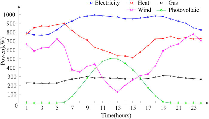
Figure 2. Predicted power of wind power, photovoltaic and loads.

Table 1

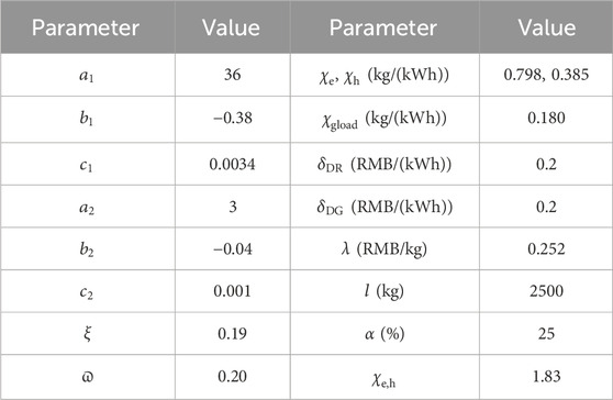
Table 1. Parameters of carbon emission calculation, carbon trading, and DR.

Table 2

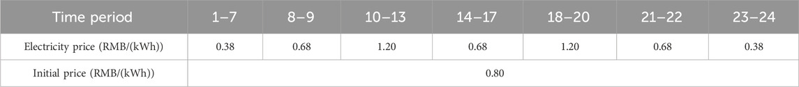
Table 2. Time-of-use electricity price.

Table 3

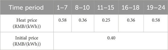
Table 3. Time-of-use heat price.

Table 4

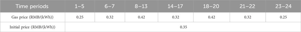
Table 4. Time-of-use gas price.

Table 5

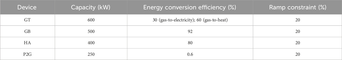
Table 5. Capacity and parameters of each device.

Table 6

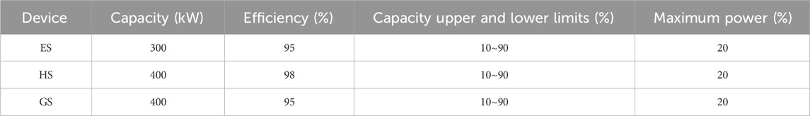
Table 6. Energy storage devices.

To compare and verify the effectiveness of the IES containing the ladder-type carbon trading mechanism and demand response proposed in this paper on the low-carbon economic operation, with the objective function of minimizing the comprehensive operation cost, the model was conducted via the YALMIP toolkit in MATLAB and solved by Gurobi solver. Six cases, as shown in Table 7 were set up.

Table 7

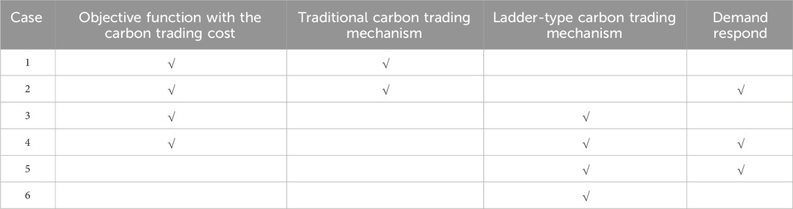
Table 7. Comparison of different cases.

The optimized scheduling results for the above six cases are shown in Table 8.

Table 8

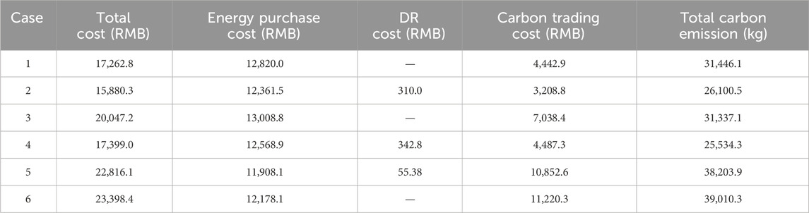
Table 8. Operation costs and actual carbon emission of IES in different cases.

6.1 Effects of the ladder-type carbon trading mechanism on the operation

6.1.1 Benefits of the ladder-type carbon trading mechanism

The effectiveness of the ladder-type carbon trading mechanism on low-carbon economic operation was compared and analyzed with cases 1, 3, and 6. Table 8 shows the highest carbon emission in case 6 as 39,010.3kg, and the carbon emission values in cases 1 and 3 are approximately 19.3% and 19.7% less than that of case 6, with case 3 reducing the carbon emission by 109.0 kg more. Case 6 has the lowest energy purchase cost of ¥12,178.1, while cases 1 and 3 have increased the cost by ¥641.9 and ¥830.7, respectively. In cases 1 and 3, case 3 carbon trading cost is approximately 58.4% more than that of case 1; in cases 3 and 6, case 6 carbon trading cost is approximately 59.4% more than that of case 3. The total cost of case 6 is the highest and that of case 1 is the lowest.

The carbon trading cost is significantly increased in case 3, leading to some decrease in carbon emission, which is approximately 0.35% less compared to that of case 1, but the total cost is 16.1% more than that of case 1. The objective function of case 6 does not consider the carbon trading cost, which causes its carbon trading cost and carbon emission to be higher, but it is mainly dominated by the energy purchase cost, and the IES primarily selects the lower-cost energy in this case, which reduces the energy purchase cost of case 6 by approximately 5.0% and 6.4% compared with cases 1 and 3, respectively. Moreover, case 6 does not pursue lower carbon emissions, which leads to its higher carbon trading cost and the highest total cost. So, the objective function considers the carbon trading cost and adopts the ladder-type carbon trading mechanism, which is beneficial to the low-carbon operation of IES.

6.1.2 Effect of changing carbon trading base price on the operation

On the basis of case 3, the base price of carbon trading is changed to explore the effect of the base price on carbon emission and the total cost of IES, as shown in Figure 3. In Figure 3, the IES’s total cost rises significantly as the carbon trading base price increases. The carbon trading base price varies in the range of ¥0.10∼¥0.60/kg, and the total cost of the IES shows an ascending trend, while the carbon emission drops extremely fast in the range of 0.10∼0.25 base price, is more stable in the range of 0.25∼0.35, and shows a slow tendency to raise after 0.35; carbon emission is minimized in the vicinity of approximately ¥0.29/kg, which is approximately 31,332.5 kg.

Figure 3

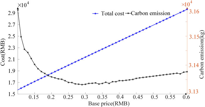
Figure 3. Effect of carbon trading base price on scheduling operation.

In case 3, the objective function includes the carbon trading cost, which is lower when the base price is lower, and the energy purchase cost becomes the dominant factor, so IES chooses energy sources with a lower cost but higher carbon emissions. As the base price increases, the extent of the impact of carbon trading cost rises, and the system chooses lower carbon energy sources in order to significantly reduce the carbon trading cost, resulting in a phenomenon of lower carbon emission. However, as the base price continues to increase, IES tries to reduce the total cost, which becomes difficult to reduce, so IES reduces the total cost by compromising some carbon emissions. Consequently, in this case, appropriately increasing the base price or choosing an optimal base price is conducive to minimizing carbon emission.

6.2 Effects of DR on the operation

6.2.1 Benefits of DR

The effectiveness of the ladder-type carbon trading mechanism on low-carbon economic operation is compared and analyzed with cases 3, 4, and 5. Table 8 shows that, for carbon emission, case 5 is the highest, case 4 is the lowest, and case 4 reduces approximately 18.5% compared to case 3. For carbon trading cost, case 4 is approximately 36.2% less than case 3. For energy purchase cost, case 5 is the lowest, and case 3 is the highest, with a decrease of approximately 3.4% for case 4 compared to case 3, and case 5 decreases by approximately 8.5% and 5.3% compared to cases 3 and 4, respectively.

In cases 3 and 4, the objective function includes the carbon trading cost, but case 4 conducts demand response. In the price-based DR stage reducing energy use in price peak periods, in the substitution-based DR stage, IES will choose both economic and low-carbon energy sources, which makes the carbon trading cost, energy purchase cost, and carbon emission less than that of case 3, and the total cost will be much lower. However, for case 5, the objective function does not include the carbon trading cost, the demand response will only consider the impact of energy purchase cost, and IES will choose more economic energy sources and ignore the carbon emission; therefore, in case 5, although the carbon emission and carbon trading cost are both larger, its energy purchase cost is the lowest among those cases. Hence, DR for the operation of IES system not only reduces carbon emission but also decreases certain energy purchase cost, which is helpful for the low-carbon economic operation of IES.

6.2.2 DR for loads of IES

Based on case 4, the IES first conducts the price-based DR for the initially predicted electricity, heat, and gas loads, as shown in Figure 4. For electricity price, the electricity demand is higher in the morning and evening peak periods, and as the price rises, in order to pursue economy, the load in the peak periods is curtailed and time-shifted to the nighttime and midday periods, which is economically efficient for the users’ energy cost. For heat prices, nighttime warming and heating demand is higher, and heat prices are higher, curtailing and time-shifting acceptable heat demand adjustment after price-based demand response. The same applies to gas load and will not be repeated.

Figure 4

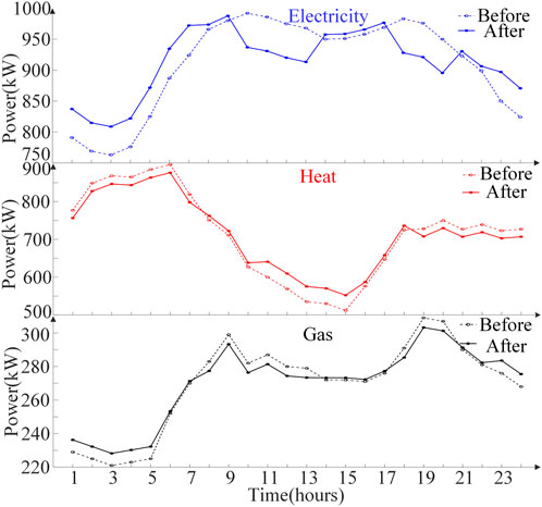
Figure 4. Price-based DR results.

The next step is to conduct substitution-based DR, as shown in Figure 5, which gives the power magnitude of the substitution conducted among the energy sources. After substitution-based DR, the system substitutes heat demand for electricity demand in time periods 1–6 and 22–24, which is due to the lower electricity price. Substituting heat demand for electricity and gas demand in time periods 7–21 is due to the higher electricity prices; heat energy needs to be generated from natural gas through GT and GB devices, and substituting it for gas demand avoids intermediate energy losses and carbon emission. All of the above is the result of the system’s comprehensive consideration of the carbon trading cost and energy purchase cost. Figures 6 and 7 show the substitution-type power for cases 2 and 5, and Figure 8 shows the three types of load curves that ultimately participate in optimal scheduling.

Figure 5

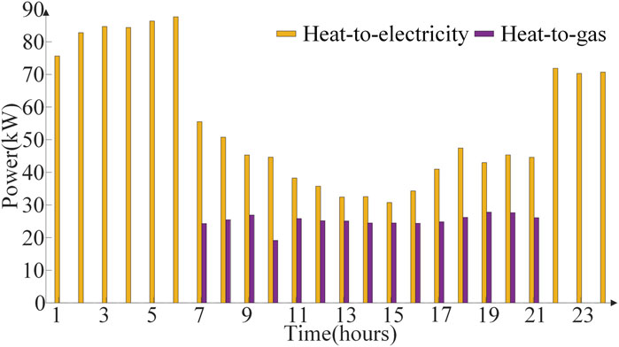
Figure 5. Substitution power for each energy source in case 4.

Figure 6

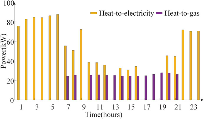
Figure 6. Substitution power for each energy source in case 2.

Figure 7

Figure 7. Substitution power for each energy source in case 5.

Figure 8

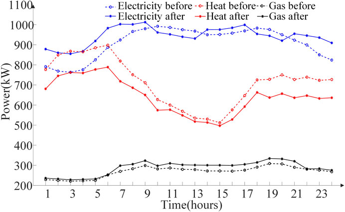
Figure 8. Demand response results.

6.2.3 DR for optimal scheduling of IES operation

Comparing cases 3 and 4, the effect of DR on each device in IES and the purchase of electricity and gas are studied, as shown in Figures 9–11. During 1–6 and 23–24 h, before DR, in order to consume the excess wind and PV power, part of electricity is used for the P2G device; however, after DR, the electricity load rises, the excess wind and PV power is consumed, and the GT output power is diminished; during the peak periods, after DR, the electricity load is decreased, and the purchased electricity power is decreased. The heat load is reduced during all periods of time after DR, decreasing the output of natural gas-consuming devices (GT and GB). After DR, there is some growth in the gas load, but there is a drop in the gas consumption of the GT and GB devices. The above plays the role of energy saving and emission reduction.

Figure 9

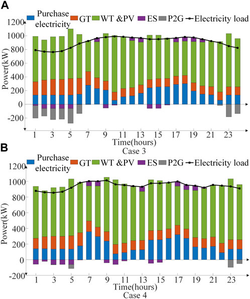
Figure 9. Electric power balance in case 3 and 4.

Figure 10

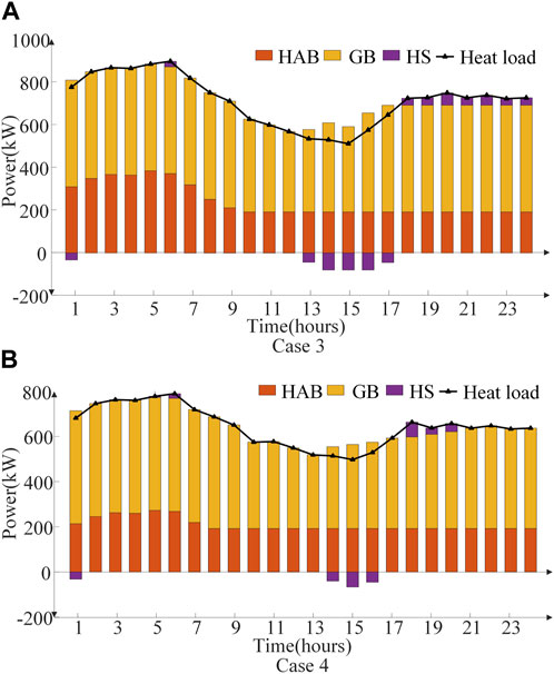
Figure 10. Heating power balance in case 3 and 4.

Figure 11

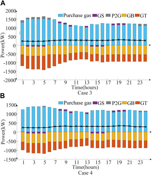
Figure 11. Gas power balance in case 3 and 4.

7 Conclusion

In the paper, an integrated energy system optimal scheduling model containing the ladder-type carbon emission trading mechanism and demand response is constructed, the original carbon emission model is improved, the carbon emission model of gas load is added, and carbon trading cost is introduced in the objective function. Price-based DR for loads is conducted by curtailing and time-shifting electric, heat, and gas loads based on their respective time-of-use prices and then utilizing the mutual substitutability of the three types of loads for substitute-based DR. The conclusions obtained are as follows:

(1) Improving the carbon emission calculation model, supplementing carbon emission of gas load, and including carbon trading cost in the objective function can reduce the carbon emission of IESs. Compared with the traditional carbon trading mechanism, the ladder-type carbon trading mechanism further reduces carbon emission by setting the interval price, and appropriately increasing the base price can achieve the lowest carbon emission.

(2) Engaging gas load in demand response and leveraging the flexibility and substitution of electricity, heat, and gas loads, demand response can further reduce the carbon emission of IESs and enable economic operation.

(3) The optimal scheduling of integrated energy systems with the ladder-type carbon trading mechanism and demand response proposed in this paper, in the day-ahead scheduling, comprehensively considers the operation objective with the energy purchase cost and carbon trading cost as the main body, which reflects its high economy and environmental protection.

The next stage of work can start from refining the two-stage operation process of the P2G device to give full play to the reuse benefit of carbon emission; furthermore, we can consider applying carbon capture and storage technology to reduce the carbon emission more efficiently and establish a highly efficient, low-carbon, and economic integrated energy system.

Data availability statement

The raw data supporting the conclusion of this article will be made available by the authors, without undue reservation.

Author contributions

LS: writing–review and editing. CL: writing–original draft and writing–review and editing. JZ: writing–review and editing. YL: conceptualization, data curation, formal analysis, funding acquisition, investigation, methodology, project administration, resources, software, supervision, validation, visualization, and writing–review and editing. JL: writing–review and editing. FW: writing–review and editing.

Funding

The author(s) declare that financial support was received for the research, authorship, and/or publication of this article. This research was funded by the project “Technology research on coordination optimization in park-oriented integrated energy system and grid interaction” (No. J2023057).

Acknowledgments

The authors are extremely grateful to each of the authors who have helped and contributed to this paper. It is their joint efforts that made this paper successfully published.

Conflict of interest

Authors JZ and JL were employed by State Grid Jiangsu Electric Power Co., Ltd.

The remaining authors declare that the research was conducted in the absence of any commercial or financial relationships that could be construed as a potential conflict of interest.

Publisher’s note

All claims expressed in this article are solely those of the authors and do not necessarily represent those of their affiliated organizations, or those of the publisher, the editors, and the reviewers. Any product that may be evaluated in this article, or claim that may be made by its manufacturer, is not guaranteed or endorsed by the publisher.

References

Chen, H., Mao, W., and Zhang, R. (2021b). Low-carbon optimal scheduling of a power system source-load considering coordination based on carbon emission flow theory. Power Syst. Prot. Control 49 (10), 1–11. doi:10.19783/j.cnki.pspc.200932

CrossRef Full Text | Google Scholar

Chen, J., Hu, Z., and Chen, J. (2021c). Optimal dispatch of integrated energy system considering ladder-type carbon trading and flexible double response of supply and demand. High. Volt. Eng. 47 (9), 3094–3106. doi:10.13336/j.1003-6520.hve.20211094

CrossRef Full Text | Google Scholar

Chen, J., Hu, Z., and Chen, Y. (2021a). Thermoelectric optimization of integrated energy system considering ladder-type carbon trading mechanism and electric hydrogen production. Electr. Power Autom. Equip. 41 (9), 48–55. doi:10.16081/j.epae.202109032

CrossRef Full Text | Google Scholar

Chen, Y., Zhu, J., and Yang, D. (2020). Research on economic optimization operation technology of park-level integrated energy system based on multi-party interest game. High. Volt. Eng. 47 (1), 102–112. doi:10.13336/j.1003-6520.hve.20200731

CrossRef Full Text | Google Scholar

Chen, Z., Zhang, Y., Tang, W., Lin, X., and Li, Q. (2019). Generic modelling and optimal day-ahead dispatch of micro-energy system considering the price-based integrated demand response. Energy 176, 171–183. doi:10.1016/j.energy.2019.04.004

CrossRef Full Text | Google Scholar

Cui, Y., Zeng, P., and Zhong, W. (2021). Low-carbon economic dispatch of electricity-gas-heat integrated energy system based on ladder-type carbon trading. Electr. Power Autom. Equip. 41 (3), 10–17. doi:10.16081/j.epae.202011030

CrossRef Full Text | Google Scholar

Hu, F., Zhou, X., and Zhang, P. (2023). Low carbon economy optimal dispatching of integrated energy system taking into account carbon capture. Acta Energiae Solaris Sin., 1–8. doi:10.19912/j.0254-0096.tynxb.2022-1832

CrossRef Full Text | Google Scholar

Huang, W., Zhang, N., Kang, C., Li, M., and Huo, M. (2019). From demand response to integrated demand response: review and prospect of research and application. Prot. Control Mod. Power Syst. 4 (1), 12–13. doi:10.1186/s41601-019-0126-4

CrossRef Full Text | Google Scholar

Kong, X., Yang, Q., and Mu, Y. (2015). Analysis method for customers demand response in time of using price. Proc. CSU-EPSA 27 (10), 75–80. doi:10.3969/j.issn.1003-8930.2015.10.12

CrossRef Full Text | Google Scholar

Li, H., Liu, D., and Yao, D. (2021a). Analysis and reflection on the development of power system towards the goal of carbon emission peak and carbon neutrality. Proc. CSEE 41 (18), 6245–6259. doi:10.13334/j.0258-8013.pcsee.210050

CrossRef Full Text | Google Scholar

Li, J., Zhu, M., and Lu, Y. (2021b). Review on optimal scheduling of integrated energy systems. Power Syst. Technol. 45 (6), 2256–2272. doi:10.13335/j.1000-3673.pst.2021.0020

CrossRef Full Text | Google Scholar

Li, P., Wang, Z., and Hou, L. (2019). Analysis of repeated game based optimal operation for regional integrated energy system. Automation Electr. Power Syst. 43 (14), 81–89. doi:10.7500/AEPS20181115007

CrossRef Full Text | Google Scholar

Li, T., Hu, Z., and Chen, Z. (2022). Multi-time scale low-carbon operation optimization strategy of integrated energy system considering electricity-gas-heat-hydrogen demand response. Electr. Power Autom. Equip. 43 (1), 16–24. doi:10.16081/j.epae.202205061

CrossRef Full Text | Google Scholar

Lu, Z., Yang, Y., and Geng, L. (2017). Low-carbon economic dispatch of the integrated electrical and heating systems based on Benders decomposition. Proc. CSEE 38 (7), 1922–1934. doi:10.7500/AEPS20170101001

CrossRef Full Text | Google Scholar

Mallapaty, S. (2020). How China could be carbon neutral by mid-century. Nature 586 (7830), 482–483. doi:10.1038/d41586-020-02927-9

PubMed Abstract | CrossRef Full Text | Google Scholar

Qin, T., Liu, H., and Wang, J. (2018). Carbon trading based low-carbon economic dispatch for integrated electricity-heat-gas energy system. Automation Electr. Power Syst. 42 (14), 8–13. doi:10.7500/AEPS20171220005

CrossRef Full Text | Google Scholar

Qu, K., Huang, L., and Yu, T. (2018). Decentralized dispatch of multi-area integrated energy systems with carbon trading. Proc. CSEE 38 (3), 697–707. doi:10.13334/j.0258-8013.pcsee.170602

CrossRef Full Text | Google Scholar

Sun, P., Hao, X., Wang, J., Shen, D., and Tian, L. (2021). Low-carbon economic operation for integrated energy system considering carbon trading mechanism. Energy Sci. Eng. 9 (11), 2064–2078. doi:10.1002/ese3.967

CrossRef Full Text | Google Scholar

Thimmapuram, P. R., and Kim, J. (2013). Consumers’ price elasticity of demand modeling with economic effects on electricity markets using an agent-based model. IEEE Trans. Smart Grid 4 (1), 390–397. doi:10.1109/tsg.2012.2234487

CrossRef Full Text | Google Scholar

Tian, F., Jia, Y., and Ren, H. (2022). Source-load" low-carbon economic dispatch of integrated energy system considering carbon capture system. Power Syst. Technol. 44 (9), 3346–3355. doi:10.13335/j.1000-3673.pst.2020.0728

CrossRef Full Text | Google Scholar

Wang, Y., Wang, Y., Huang, Y., Yang, J., Ma, Y., Yu, H., et al. (2019). Operation optimization of regional integrated energy system based on the modeling of electricity-thermal-natural gas network. Appl. Energy 251, 113410. doi:10.1016/j.apenergy.2019.113410

CrossRef Full Text | Google Scholar

Wei, Z., Ma, X., and Guo, Y. (2022). Optimized operation of integrated energy system considering demand response under carbon trading mechanism. Electr. Power Constr. 43 (1), 1–9. doi:10.12204/j.issn.1000-7229.2022.01.001

CrossRef Full Text | Google Scholar

Wei, Z., Zhang, S., and Sun, G. (2016). Carbon trading based low-carbon economic operation for integrated electricity and natural gas energy system. Automation Electr. Power Syst. 40 (15), 9–16. doi:10.7500/AEPS20151109004

CrossRef Full Text | Google Scholar

Yun, B., Zhang, E., and Zhang, G. (2022). Optimal operation of an integrated energy system considering integrated demand response and a “dual carbon” mechanism. Power Syst. Prot. Control 50 (22), 11–19. doi:10.19783/j.cnki.pspc.220621

CrossRef Full Text | Google Scholar

Zhang, S., Wang, D., and Cheng, H. (2022). Key technologies and challenges of low-carbon integrated energy system planning for carbon emission peak and carbon neutrality. Automation Electr. Power Syst. 46 (8), 189–207. doi:10.7500/AEPS20210703002

CrossRef Full Text | Google Scholar

Zhang, T., Guo, Y., and Li, Y. (2021). Optimization scheduling of regional integrated energy systems based on electric-thermal-gas integrated demand response. Power Syst. Prot. Control 49 (1), 52–61. doi:10.19783/j.cnki.pspc.200167

CrossRef Full Text | Google Scholar

Zhao, G., Ding, Q., and Fu, J. (2021). Research on the low-carbon implementation path of regional energy system relying on the linkage mechanism of multi-markets. Electr. Power Constr. 42 (3), 19–26. doi:10.12204/j.issn.1000-7229.2021.03.003

CrossRef Full Text | Google Scholar