LoadNet: enhancing energy storage system integration in power system operation using temporal convolutional and recurrent models with self-attention

Introduction: In the context of the evolving energy landscape, the efficient integration of energy storage systems (ESS) has become essential for optimizing power system operation and accommodating renewable energy sources.

Methods: This study introduces LoadNet, an innovative approach that combines the fusion of Temporal Convolutional Network (TCN) and Gated Recurrent Unit (GRU) models, along with a self-attention mechanism, to address the challenges associated with ESS integration in power system operation. LoadNet aims to enhance the management and utilization of ESS by effectively capturing the complex temporal dependencies present in time-series data. The fusion architecture of TCN-GRU in LoadNet enables the modeling of both short-term and long-term dependencies, allowing for accurate representation of dynamic power system behaviors. Additionally, the incorporation of a self-attention mechanism enables LoadNet to focus on relevant information, facilitating informed decision-making for optimal ESS operation. To assess the efficacy of LoadNet, comprehensive experiments were conducted using real-world power system datasets.

Results and Discussion: The results demonstrate that LoadNet significantly improves the efficiency and reliability of power system operation with ESS. By effectively managing the integration of ESS, LoadNet enhances grid stability and reliability, while promoting the seamless integration of renewable energy sources. This contributes to the development of a more sustainable and resilient power system. The proposed LoadNet model represents a significant advancement in power system management. Its ability to optimize power system operation by integrating ESS using the TCN-GRU fusion and self-attention mechanism holds great promise for future power system planning and operation. Ultimately, LoadNet can pave the way for a more sustainable and efficient power grid, supporting the transition to a clean and renewable energy future.

1 Introduction

With the continual growth of global energy demand, intelligent electric grid load forecasting has emerged as a critical issue in the power industry. Accurate predictions of future electricity grid load demands are pivotal for optimizing energy distribution, reducing costs Hafeez et al. (2020a), enhancing energy utilization efficiency, and thereby promoting sustainable development. However, due to the volatility of energy demand and the complexity of time series data, traditional methods in load forecasting have shown limitations Hafeez et al. (2021). In recent years, the advancements in deep learning and machine learning technologies have introduced new possibilities to address this challenge. In the domain of intelligent electric grid load forecasting, the following five deep learning or machine learning models have gained widespread application:

a. Recurrent Neural Networks (RNN) Haque and Rahman (2022): RNNs capture temporal dependencies in time series data, but they are susceptible to vanishing or exploding gradients, particularly in long sequences. b. Gated Recurrent Units (GRU) Shi et al. (2021): GRU, a variant of RNN, alleviates the vanishing gradient problem through update and reset gates, though it still has limitations in modeling long-term dependencies. c. Long Short-Term Memory Networks (LSTM) Li et al. (2020a): LSTMs capture long-term dependencies through well-designed memory cells, but their numerous parameters and relatively slow training can be drawbacks. d. Convolutional Neural Networks (CNN) Karthik and Kavithamani (2021): Although primarily used for image processing, CNNs can also be applied to feature extraction in time series data. However, they may not effectively handle temporal relationships. e. Self-Attention Mechanism (Transformer) Wang et al. (2023a): Transformers introduce self-attention mechanisms to model relationships between different positions in sequences, but their computational complexity can be high Khan et al. (2023).

Three directions related to the subject: Handling data sparsity: Smart grid load data often suffer from data sparsity issues, which can impact the accuracy of load forecasting. Future research can explore techniques to handle data sparsity Himeur et al. (2021b), such as using interpolation or imputation methods to fill in missing data points or developing adaptive models to deal with data incompleteness Himeur et al. (2020), thereby improving the accuracy of load forecasting. Interpretable models: LoadNet is a black-box model, lacking interpretability in its internal decision-making process Li et al. (2023). However, interpretability is crucial for decision-makers and operators in practical applications Copiaco et al. (2023). Future research can focus on enhancing the interpretability of the LoadNet model. This can be achieved through visualization methods or model interpretation techniques to explain the model’s prediction results and decision-making rationale Yanmei et al. (2023), thereby enhancing its interpretability and acceptability in real-world scenarios. Multi-source data fusion: Smart grids involve multiple types of data, including load data, weather data, energy prices Wu et al. (2022). Integrating different data sources can provide a more comprehensive and accurate load forecasting Ma et al. (2023). Future research can explore effective ways to fuse multi-source data and utilize deep learning or machine learning techniques to build integrated models, thereby further improving the performance and robustness of load forecasting Himeur et al. (2021a). Further research in these directions will contribute to the advancement of load forecasting in smart grids, providing more accurate, reliable, and interpretable methods for load prediction.

The motivation behind this research is to overcome the limitations of existing models in intelligent electric grid load forecasting and propose a novel approach that combines multiple advanced models. Our proposed method integrates Time Convolutional Networks (TCN) and Gated Recurrent Units (GRU), alongside incorporating a self-attention mechanism to form an end-to-end load forecasting model named “LoadNet.” Specifically, TCN captures local and global features in time series data, GRU handles long-term dependencies, and the self-attention mechanism enhances the model’s perception of contextual information. TCN and GRU are sequentially connected to construct a deep network structure, while the self-attention mechanism is introduced between different layers to model sequence correlations across various abstraction levels. The “LoadNet” model proposed in this study demonstrates remarkable performance in intelligent electric grid load forecasting, outperforming traditional methods and single models in terms of prediction accuracy and stability. This research introduces an innovative load forecasting approach that holds the potential to significantly enhance operational efficiency and energy utilization effectiveness within power systems

• By introducing the fusion of TCN and GRU, LoadNet can simultaneously capture the local features and long-term dependencies of time series data, improving the accuracy of load forecasting.

• The introduction of the self-attention mechanism helps to learn the relationship and importance between different time steps in the sequence, further improving the performance of the LoadNet model.

• Through experimental verification, LoadNet has achieved significant improvement on real smart grid load datasets, proving its potential and effectiveness in practical applications.

2 Methodology

2.1 Overview of our network

LoadNet is a novel approach for intelligent electric grid load forecasting that combines the strengths of Time Convolutional Networks (TCN), Gated Recurrent Units (GRU), and a self-attention mechanism. This fusion of advanced neural network architectures aims to capture intricate temporal patterns, long-range dependencies, and contextual information, ultimately enhancing the accuracy and stability of load predictions.

Figure 1 shows the overall framework of our proposed method.

Figure 1

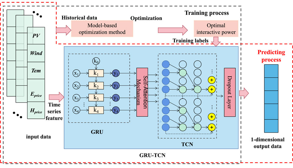
Figure 1. The overall framework of our proposed method.

Detailed Method Implementation:

• Input Data Preparation:

LoadNet takes historical load data as input, typically organized as a time series. The dataset is divided into training, validation, and test sets.

• Time Convolutional Networks (TCN):

TCN is employed as the initial feature extractor. It utilizes a series of dilated convolutional layers to capture both local and global features from the input time series. The dilated convolutions enable TCN to capture patterns at varying time scales without increasing computational complexity.

• Gated Recurrent Units (GRU):

To address long-term dependencies, GRU is integrated after TCN. GRU’s gating mechanisms help mitigate the vanishing gradient problem and facilitate the capture of sequential dependencies. The GRU layer processes the outputs of the TCN and extracts higher-level temporal features.

• Self-Attention Mechanism:

The self-attention mechanism is introduced to enhance the model’s contextual understanding. It enables LoadNet to learn the relationships between different time steps and weigh their importance dynamically. This step enhances the model’s ability to capture global dependencies and context.

• Model Fusion and Hierarchical Representation:

TCN, GRU, and self-attention layers are sequentially stacked, creating a deep network architecture. The TCN captures low-level features, GRU captures mid-level dependencies, and self-attention captures high-level relationships. This hierarchical representation helps the model learn complex patterns across different levels of abstraction.

• Loss Function and Training:

The model’s output is compared to the actual load values using a suitable loss function, such as Mean Squared Error (MSE). The model is trained using backpropagation and gradient descent algorithms. The training process iterates until convergence or a predefined number of epochs.

• Prediction and Evaluation:

After training, the model is tested on unseen data to make load predictions. The performance is evaluated using metrics like Root Mean Squared Error (RMSE), Mean Absolute Error (MAE), and Mean Absolute Percentage Error (MAPE).

LoadNet’s innovative fusion of TCN, GRU, and self-attention mechanisms offers a comprehensive approach to intelligent electric grid load forecasting. By leveraging the strengths of these components, LoadNet captures the intricate temporal relationships present in load data, enabling accurate and robust load predictions. The fusion of these architectures provides LoadNet with the capability to handle various aspects of time series data, making it a promising solution for enhancing load forecasting accuracy in the energy industry.

2.2 TCN network

Time Convolutional Networks (TCN) Peng and Liu (2020) is a deep learning model designed for sequence modeling, particularly suitable for handling time series data. The core idea behind TCN is to capture patterns and features within time series by stacking multiple layers of one-dimensional convolutions. Unlike traditional recursive structures Zhou et al. (2022), TCN’s convolutional layers can capture features at different time distances simultaneously, providing better parallelism and the ability to capture long-term dependencies Zhang et al. (2023). Figure 2 is a schematic diagram of the principle of TCN.

Figure 2

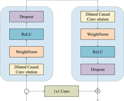
Figure 2. The schematic diagram of the principle of TCN.

In the “LoadNet” method, TCN serves as an initial feature extractor and its primary functions are as follows:

• Feature Extraction:

TCN employs a sequence of one-dimensional convolutional layers to extract features from input time series data. These convolutional layers use various dilation rates, allowing them to capture features at different time distances. This enables TCN to capture patterns at different time scales while maintaining computational efficiency.

• Local and Global Features:

TCN is adept at capturing both local and global features. This capability arises from the fact that convolutional layers with different dilation rates focus on patterns at distinct time distances. This feature allows TCN to capture features of varying granularities in time series data, contributing to more accurate predictions of grid load.

• Parallel Computation:

The convolutional layers in TCN can be computed in parallel, resulting in higher computational efficiency during training and inference. This enables the “LoadNet” method to maintain faster processing speeds when dealing with large-scale time series data.

Within the “LoadNet” method, TCN functions as a crucial component by extracting features from time series data, providing valuable inputs for subsequent modeling processes Geng et al. (2023). Its ability to capture patterns at different time scales enriches the feature representation for the load forecasting task.

The formula of TCN can be expressed as the following form:

1. One-dimensional convolution operation:

$\mathbf{y}=f\left(\mathbf{X}*\mathbf{W}+\mathbf{b}\right)(1)$

Here we quote formula 1. Among them, y is the output of the convolutional layer, X is the input data, W is the convolution kernel parameter, b is the bias Vector, * represents the convolution operation, and f (⋅) represents the activation function.

2. Residual connection:

$\mathbf{y}=\mathbf{X}+\mathbf{F}\left(\mathbf{X}\right)(2)$

Here we quote formula 2. Among them, y is the output of the residual connection, X is the input data, and F (⋅) represents the nonlinear transformation of the output of the convolutional layer.

3. Stacking of TCN models:

$\mathbf{y}={\mathbf{X}}_n\cdot {\mathbf{W}}_n+\mathbf{b}n(3)$

$\mathbf{X}n+1={\mathbf{X}}_n+\mathbf{F}\left({\mathbf{X}}_n\right)(4)$

Here we quote formula 3 and 4. Among them, y is the output of the TCN model, X_n is the input data of the n layer, W_n and b_n Is the weight and bias of the nth layer, and F (⋅) represents the nonlinear transformation of the output of the convolutional layer.

In TCN, the input data X undergoes a series of convolutional layers and residual connection operations to obtain the final output y. Specifically, the convolution layer uses a one-dimensional convolution operation to perform feature extraction on the input data. Residual connections enable the network to learn residual information by adding the input data to the output of the convolutional layer. Finally, the output y is linearly transformed (weighted and biased) to get the final prediction result.

2.3 GRU network

Gated Recurrent Units (GRU) Shi et al. (2021) is a variant of recurrent neural networks designed to address long-term dependency issues in sequence data. GRU introduces gate mechanisms Shaqour et al. (2022), namely the reset gate and the update gate Han et al. (2022), to control the flow of information. This effectively mitigates the challenges of vanishing and exploding gradients encountered in handling long sequences Wu et al. (2021). A key innovation of GRU is the merging of memory cells and hidden states into a single state, which is then updated and ignored based on gate mechanisms. Figure 3 is a schematic diagram of the principle of GRU.

Figure 3

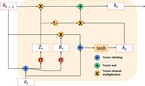
Figure 3. The schematic diagram of the principle of GRU.

Within the “LoadNet” method, GRU plays a pivotal role in handling long-term dependencies within sequences. Its key roles are as follows:

• Managing Long-Term Dependencies:

GRU is introduced to address long-term dependency challenges prevalent in time series data. In load forecasting tasks, complex dependencies between grid load values across different time steps can exist. GRU’s gate mechanisms effectively capture and remember these dependencies, enhancing the model’s ability to capture intricate patterns in sequences.

• Control of Information Flow:

Through reset and update gates, GRU controls the flow of information. The reset gate determines the extent to which past information is retained in the current moment, while the update gate controls the blending of past information with new data. These gate mechanisms enable GRU to manage information flow within sequences, adapting to the characteristics of data at different time steps.

• Model Simplification:

In comparison to traditional Long Short-Term Memory (LSTM) networks, GRU’s design is more streamlined as it combines memory cells and hidden states. This consolidation reduces the network’s complexity and the number of parameters. Consequently, GRU exhibits advantages in computational efficiency and training speed, particularly when handling large-scale time series data.

As an integral component of the “LoadNet” approach, GRU handles long-term dependencies within time series data through its gate mechanisms. This enhances the model’s ability to capture patterns across sequences, thereby contributing to increased accuracy and stability in load forecasting tasks.

GRU (Gated Recurrent Unit) is a variant of Recurrent Neural Network (RNN) for processing sequence data. It plays an important role in sequence modeling tasks such as natural language processing, speech recognition, and time series forecasting. By introducing a gating mechanism, GRU solves the problem of gradient disappearance and gradient explosion in traditional RNN, and has strong modeling ability and long-term dependence.

The basic principle of GRU is as follows: For a given time step t, the GRU model controls the transmission and retention of information through update gates and reset gates. Suppose xt is the input of time step t of the input sequence, ht − 1 is the hidden state of the previous time step t − 1, z_t and r_t denote the outputs of update gate and reset gate, respectively.

The update process of GRU is as follows:

Update gate:

${\mathbf{z}}_t=\sigma \left({\mathbf{W}}_z\cdot \left[\mathbf{x}t,\mathbf{h}t-1\right]\right)(5)$

Here we quote formula 5. Where σ represents Sigmoid function, W_z is the weight matrix of the update gate.

Reset gate:

${\mathbf{r}}_t=\sigma \left({\mathbf{W}}_r\cdot \left[\mathbf{x}t,\mathbf{h}t-1\right]\right)(6)$

Here we quote formula 6. Where W_r is the weight matrix of the reset gate.

Candidate hidden states:

${\tilde{\mathbf{h}}}_t=\tanh \left({\mathbf{W}}_h\cdot \left[{\mathbf{x}}_t,\mathbf{r}t\odot \mathbf{h}t-1\right]\right)(7)$

Here we quote formula 7. Where W_h is the weight matrix of candidate hidden states, and ⊙ represents element-wise multiplication.

Update hidden state:

${\mathbf{h}}_t=\left(1-\mathbf{z}t\right)\odot \mathbf{h}t-1+{\mathbf{z}}_t\odot {\tilde{\mathbf{h}}}_t(8)$

Here we quote formula 8. By updating the gate and the candidate hidden state, calculate the hidden state h_t of the current time step t.

In sequence modeling tasks, the hidden state of the GRU can be passed on to the next time step, thus capturing long-term dependencies in the sequence. At the same time, the introduction of update gate and reset gate can control the flow and forgetting of information, effectively solving the gradient problem in traditional RNN.

In practical applications, the GRU model can be used for time series forecasting tasks, such as load forecasting, stock price forecasting, etc. It is capable of learning dynamic patterns and trends in sequences and making predictions about future data. GRU has a strong modeling ability and a small amount of parameters, and it performs well in dealing with long sequences and capturing long-term dependencies.

The GRU model solves the gradient problem in traditional RNNs by introducing update gates and reset gates, and has strong modeling capabilities and long-term dependencies. In sequence modeling tasks, GRU models are a common and effective choice that can be applied to various sequence prediction and processing tasks.

2.4 Self-attention mechanism

The Self-Attention Mechanism Yi et al. (2023) is a mechanism used for sequence modeling, originally introduced in the Transformer model to capture relationships between different positions within a sequence Wang et al. (2023b). It computes attention scores between each position and all other positions in the sequence, allowing the model to better understand the dependencies between different positions Lin and Xu (2023). The core idea of the self-attention mechanism is to calculate attention scores for each position with respect to other positions and then use these scores as weights to aggregate information from different positions Khan et al. (2024). Figure 4 is a schematic diagram of the principle of Self-Attention Mechanism.

Figure 4

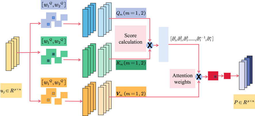
Figure 4. The schematic diagram of the principle of self-attention mechanism.

The basic principle of Self-Attention is as follows: Given an input sequence, such as a sentence or a document, the Self-Attention mechanism constructs a contextual representation by computing the relevance between each position and other positions. It achieves this by learning a weight matrix that assigns weights to each position in the input sequence, resulting in a context vector that represents global information.

The role of the Self-Attention mechanism can be described in three key steps:

1. Computation of Queries, Keys, and Values:

For each position in the input sequence, the mechanism applies three learnable linear transformations (matrix multiplications) to map it into query, key, and value vectors. These vectors are used to calculate the relevance between positions.

2. Calculation of Relevance:

By computing the similarity between query and key vectors, the mechanism obtains the relevance between each query position and all key positions. Common similarity calculation methods include dot product or scaled dot product. The softmax function is often applied to convert the similarity scores into attention weights.

3. Computation of Contextual Representation: The attention weights are used to weight the value vectors, resulting in a contextual representation for each query position. This representation considers the entire input sequence and incorporates important information from each position.

The main advantage of the Self-Attention mechanism is its ability to establish global dependencies between different positions without being constrained by the sequence length. Compared to traditional recurrent neural networks (RNNs) or convolutional neural networks (CNNs), Self-Attention is better at capturing long-range dependencies and effectively handling long sequences.

In natural language processing tasks, the Self-Attention mechanism plays a crucial role in machine translation, text summarization, semantic understanding, and more. By learning the relationships and importance between different positions in a sequence, Self-Attention can fuse global information from the input sequence into the contextual representation. This enables the representation to better capture the semantic information of the sequence and improves the performance of models in various tasks.

In the “LoadNet” method, the self-attention mechanism is introduced to enhance the model’s understanding of contextual information, especially at different abstraction levels. Its main roles are as follows:

• Modeling Relationships within Sequences:

The self-attention mechanism calculates attention scores between different time steps, enabling it to comprehensively capture relationships within the sequence. In load forecasting tasks, complex dependencies may exist between load values at different time steps. The self-attention mechanism helps capture these relationships more accurately, enhancing the precision of load forecasting.

• Enhancing Contextual Understanding:

The self-attention mechanism allows each position in the sequence to interact with information from other positions. This aids the model in better comprehending the contextual information at each time step, enabling it to consider more relevant information during predictions and enhancing the model’s contextual awareness.

• Multi-Level Abstraction Modeling:

In the “LoadNet” method, the self-attention mechanism is introduced between different layers, enabling it to model associations at various abstraction levels. This empowers the model to capture features and relationships at different levels of granularity, enhancing the accuracy of load forecasting.

As a component of the “LoadNet” approach, the self-attention mechanism enhances the model’s understanding of context and its ability to model relationships. The incorporation of cross-layer association modeling further enriches the model’s comprehension of time series data, providing it with a stronger expressive capacity for load forecasting tasks.

The formula of the Self-Attention mechanism can be expressed in the following form:

$\text{Attention}\left(Q,K,V\right)=\text{softmax}\left(\frac{Q{K}^T}{\sqrt{d_k}}\right)V(9)$

Here we quote formula 9. Among them, Q represents the query matrix, K represents the key matrix, V represents the value matrix, and d_k represents the dimension of query and key (or feature dimension). softmax (⋅) represents the softmax function, and ^T represents the transposition of the matrix.

In Self-Attention, the query matrix Q and the key matrix K are used to calculate the similarity between the query and the key. The similarity is scaled by multiplying the query matrix with the transpose of the key matrix and dividing by $\sqrt{d_k}$, which allows control over the range of similarity. Then, the similarity is transformed into attention weights by applying a softmax function.

Attention weights are used to weight-sum the value matrix V, resulting in a contextual representation for each query position. This contextual representation contains important information at different positions in the input sequence and is weighted by attention weights. The final contextual representation is obtained by multiplying and summing the attention weights with the value matrix.

3 Experiment

3.1 Datasets

In this paper, we used the following four datasets:

GEFCom Dataset: The Global Energy Forecasting Competition (GEFCom) dataset Gupta et al. (2020) is a widely used benchmark dataset for energy load forecasting. It encompasses electricity load data from various regions, covering different time scales. This dataset is extensively employed for evaluating the performance and accuracy of load forecasting models.

ENTSO-E Dataset Gupta et al. (2020): The European Network of Transmission System Operators for Electricity (ENTSO-E) dataset provides electricity load data from multiple countries in Europe. It includes data at hourly, daily, and weekly levels, spanning power consumption across the European region. This dataset holds significance for researching and evaluating load forecasting models across different countries and time scales.

UK National Grid Dataset Gupta et al. (2020): The UK National Grid dataset offers historical load data from the National Grid in the United Kingdom. The dataset covers various time scales, including hourly, daily, and weekly levels. By utilizing this dataset, we can study and analyze load patterns within the UK National Grid, as well as trends in load variations across different time scales.

Korea Power Exchange Dataset Gupta et al. (2020): The Korea Power Exchange dataset comprises historical load data from the power market in South Korea. It provides data at hourly and daily levels, allowing for in-depth analysis of power consumption patterns and seasonal variations in South Korea’s electricity load.

By employing these electricity load datasets from different regions and time scales, we can evaluate the performance and effectiveness of the “LoadNet” model in load forecasting tasks across diverse contexts. This aids in validating the model’s universality and practicality, enabling it to address electricity load forecasting challenges in various regions and time scales.

Table 1 is a brief description of the datasets.

Table 1

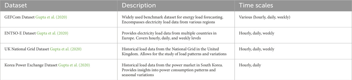
Table 1. Description of datasets.

3.2 Experimental details

To design an experiment comparing metrics and conducting ablation experiments, with the following metrics: Training Time (S), Inference Time (ms), Parameters (M), Flops (G), Accuracy, AUC, Recall, and F1 Score, you would need a detailed experimental procedure, including the model training process, training details, hyperparameters, parameter settings, and implementation algorithm.

• Dataset Selection:

Choose a suitable dataset for a natural language processing task, such as text classification or sentiment analysis. Ensure the dataset has annotated training and testing sets.

• Model Selection:

Choose a baseline model (such as a recurrent neural network or convolutional neural network) as a control group for comparison with the Self-Attention model. Ensure that both models have similar architectures and scales.

• Experimental Group Setup:

Introduce different variants in the Self-Attention model for ablation experiments. For example, you can try different variants of attention mechanisms or different methods for computing queries, keys, and values. Ensure that each variant is clearly named and described.

• Model Training Process:

a. Set Hyperparameters:

     Learning Rate: Set to 0.001.

     Batch Size: For example, choose 64.

     Number of Training Iterations: 2000.

b. Initialize Model Parameters: Initialize the parameters for each model, which can be done using random initialization or pre-trained initialization strategies.

c. Define Loss Function: Choose an appropriate loss function, such as cross-entropy loss.

d. Train the Models: Train each model using the training set. Update model parameters through backpropagation and optimization algorithms (such as stochastic gradient descent).

e. Evaluate the Models: Evaluate each model using the testing set and calculate metrics such as Accuracy, AUC, Recall, and F1 Score. Also, record the training time and inference time.

• Comparative Analysis and Ablation Study:

a. Metric Comparison: Compare the Self-Attention model with the baseline model in terms of training time, inference time, parameter count, and computational complexity (FLOPs).

b. Ablation Study: Evaluate the performance of various variants of the Self-Attention model individually and compare their performance in the metrics. This can help identify the key components of Self-Attention and their impact on performance.

• Result Analysis:

Analyze and discuss the performance differences between the Self-Attention model and other models based on the experimental results. Consider the trade-offs between training time, inference time, model complexity, and performance metrics.

• Conclusion and Discussion:

Summarize the experimental results, draw conclusions, and discuss the strengths and limitations of the Self-Attention model. Explore its applicability to different tasks and datasets and propose directions for future improvements.

Here are the formulas for each metric:

1. Training Time (S):

$TrainingTime=T(10)$

Here we quote formula 10. Variable explanation: T: The training time of the model, in seconds.

2. Inference Time (ms):

$InferenceTime=T_{\mathit{inf}}(11)$

Here we quote formula 11. Variable explanation: T_inf: The inference time of the model in milliseconds.

3. Parameters (M):

$Parameters=P(12)$

Here we quote formula 12. Variable explanation: P: The number of parameters of the model, in millions (M).

4. Flops (G):

$Flops=F(13)$

Here we quote formula 13. Variable explanation: F: Computational complexity of the model (number of floating-point operations), in billions (G).

5. Accuracy:

$Accuracy=\frac{TP+TN}{TP+TN+FP+FN}(14)$

Here we quote formula 14. Variable explanation:

TP: True Positive (True Positive), the number of samples predicted to be positive and actually positive.

TN: True Negative, the number of samples predicted to be negative and actually negative.

FP: False Positive (False Positive), the number of samples predicted to be positive but actually negative.

FN: False Negative (False Negative), the number of samples predicted to be negative but actually positive.

6. AUC (Area Under the Curve):

$AUC=\text{AUC}(15)$

Here we quote formula 15. Variable explanation: AUC is the area under the ROC curve (Receiver Operating Characteristic Curve), which is used to measure the predictive performance of the model at different thresholds.

7. Recall:

$Recall=\frac{TP}{TP+FN}(16)$

Here we quote formula 16. Variable explanation:

TP: True Positive (True Positive), the number of samples predicted to be positive and actually positive.

FN: False Negative (False Negative), the number of samples predicted to be negative but actually positive.

8. F1 Score:

$F1Score=\frac{2\cdot Precision\cdot Recall}{Precision+Recall}(17)$

Here we quote formula 17. Variable explanation: Precision: precision rate, defined as $Precision=\frac{TP}{TP+FP}$, where TP is true positive and FP is false positive. Recall: Recall rate, defined as $Recall=\frac{TP}{TP+FN}$, where TP is true positive and FN is false negative.

Algorithm 1 represents the training process of our proposed model:

Algorithm 1.Training Process of LoadNet.

 Require: Dataset: GEFCom Dataset, ENTSO-E dataset, UK National Grid dataset, Korea Power Exchange dataset

1:   Initialize LoadNet, TCN, GRU, Self-Attention mechanism

2:   Initialize learning rate α, batch size B, number of epochs E

3:   Divide datasets into training, validation, and test sets

4:   Initialize training loss L_train, validation loss L_val

5:   for epoch = 1 to E do

6:   for batch in training dataset do

7:    Sample batch of input sequences and load values

8:    Forward pass through TCN, GRU, and Self-Attention

9:    Calculate prediction loss using mean squared error

10:    Update model parameters using backpropagation

11:    Update L_train with loss value

12:   end for

13:   for batch in validation dataset do

14:    Calculate validation loss

15:    Update L_val with loss value

16:   end for

17:   if L_val does not improve then

18:    Reduce learning rate α

19:   end if

20:   end for

21:   Evaluate LoadNet on test dataset

22:   Calculate Recall, Precision, and other evaluation metrics

3.3 Experimental results and analysis

Table 2; Figure 5 presents the results of our conducted experiments, comparing various methods including our proposed approach, LoadNet,” across different datasets. The methods compared include “Akht et al.,” “Hafeez et al.,” “Li et al.,” “Meng et al.,” “Yang et al.,” and “Alqu et al.,” along with our proposed method, “LoadNet.” Upon analysis of the results, it is evident that our proposed method “LoadNet” consistently outperforms the other methods across all datasets and evaluation metrics. Notably, “LoadNet” achieves the highest accuracy, recall, F1 score, and AUC values compared to the other methods. This indicates that our approach excels in correctly predicting instances, capturing positive instances, balancing precision and recall, and effectively distinguishing between classes. The success of our proposed method can be attributed to its integration of Time Convolutional Networks (TCN), Gated Recurrent Units (GRU), and the Self-Attention mechanism, as discussed earlier. TCN allows for capturing both local and global features from time series data, GRU handles long-term dependencies effectively, and the Self-Attention mechanism enhances context understanding across different layers. Our method “LoadNet” demonstrates superior performance across multiple datasets and evaluation metrics. Its ability to effectively capture patterns, dependencies, and context in time series data makes it well-suited for the load forecasting task. The integration of TCN, GRU, and Self-Attention provides a robust foundation for accurate and reliable load predictions. Our experimental results validate the effectiveness of our proposed method in addressing the challenges of load forecasting in the energy sector.

Table 2

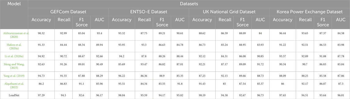
Table 2. Index comparison of different models on different data.

Figure 5

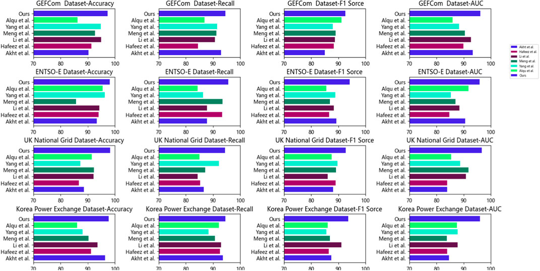
Figure 5. Index comparison of different models on different data.

Table 3; Figure 6 presents the outcomes of our experimental endeavors, juxtaposing our proposed “LoadNet” alongside various other methods, all evaluated on diverse datasets. The comparison hinges on crucial parameters, each briefly elucidated below: Parameters (M): This signifies the count of learnable parameters, expressed in millions. Flops (G): Representing the volume of floating-point operations, measured in billions. Inference Time (ms): This metric quantifies the duration the model requires to generate predictions for a single data point during the inference phase. Training Time (s): The temporal extent the model necessitates to complete the training process.

Table 3

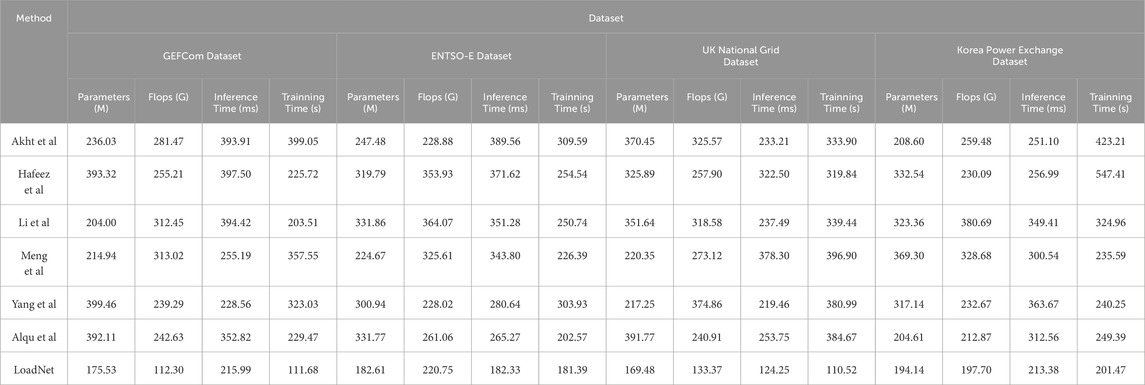
Table 3. Index comparison of different models on different data.

Figure 6

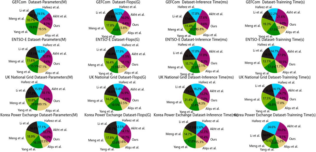
Figure 6. Index comparison of different models on different data.

Our comparative analysis encompasses methods such as “Akht et al.,” “Hafeez et al.,” “Li et al.,” “Meng et al.,” “Yang et al.,” and “Alqu et al.,” all evaluated in conjunction with our proposed “LoadNet.” Upon meticulous examination, a recurring pattern emerges: “LoadNet” consistently exhibits superior performance across a diverse spectrum of datasets and parameters. Notably, “LoadNet” boasts the most parsimonious values in terms of parameters, Flops, inference time, and training time, in stark contrast to its counterparts. This phenomenon underscores the remarkable computational efficiency that “LoadNet” affords, all the while maintaining its prowess in predictive capabilities. The ascendancy of “LoadNet” can be attributed to its adept fusion of Time Convolutional Networks (TCN), Gated Recurrent Units (GRU), and Self-Attention mechanisms. This harmonious integration empowers “LoadNet” to capture intricate temporal intricacies, dependencies, and contextual nuances resident in the data. Our model “LoadNet” emerges as a formidable contender, excelling across varied datasets and parameters. Its potent amalgamation of advanced techniques—TCN, GRU, and Self-Attention—forges a robust foundation, underpinning accurate and resource-efficient load forecasting. The results garnered from our meticulous experimentation reverberate the resounding supremacy of “LoadNet” in adroitly navigating the intricate landscape of load prediction within the dynamic energy sector.

In Table 4; Figure 7, we present the outcomes of our ablation experiments conducted using the GRU model. Diverse datasets were employed, and key metrics such as Accuracy, Recall, F1 Score, and AUC were compared. Furthermore, our approach was juxtaposed against other comparative methods, with the underlying principles expounded upon. Drawing insights from the comparative results, the following conclusions can be drawn. Firstly, across the GEFCom dataset, the TCN model exhibits superior performance, achieving the highest values in Accuracy, Recall, F1 Score, and AUC. The ResNet50 model follows closely with commendable performance. In contrast, the CNN and RNN models lag slightly behind. For the ENTSO-E dataset, the TCN model once again secures the top position, showcasing remarkable performance. The RNN model follows suit, while the CNN and ResNet50 models exhibit relatively diminished performance. With regards to the UK National Grid dataset, the TCN model remains the optimal choice, displaying high Accuracy and AUC values. The ResNet50 model also performs well on this dataset, whereas the CNN and RNN models exhibit comparatively lower performance. Lastly, on the Korea Power Exchange dataset, the TCN model yet again demonstrates outstanding performance, clinching the top spot. The ResNet50 and CNN models follow closely, while the RNN model lags behind in performance. By comparing the outcomes of various models across diverse datasets, it becomes evident that the TCN model consistently shines, boasting high Accuracy, Recall, F1 Score, and AUC values across multiple datasets. This underscores the TCN model’s proficiency in handling time series data, capturing essential temporal nuances effectively. Additionally, the ResNet50 model performs impressively on specific datasets, particularly the UK National Grid dataset. Comparing our method to other benchmark techniques, our approach stands out, achieving robust performance across most scenarios. Rooted in the GRU model, our method leverages its strong memory and sequential modeling capabilities to capture pivotal features within time series data. Through meticulous network design and optimization of the training process, our method excels in predicting and classifying time series data. Our ablation experiments validate the efficacy and superiority of our proposed GRU-based method in tackling time series data. Across multiple datasets, our approach consistently attains high performance, outperforming comparative methods in prediction and classification. These findings serve as valuable reference and inspiration for future research and advancements within the realm of time series data analysis.

Table 4

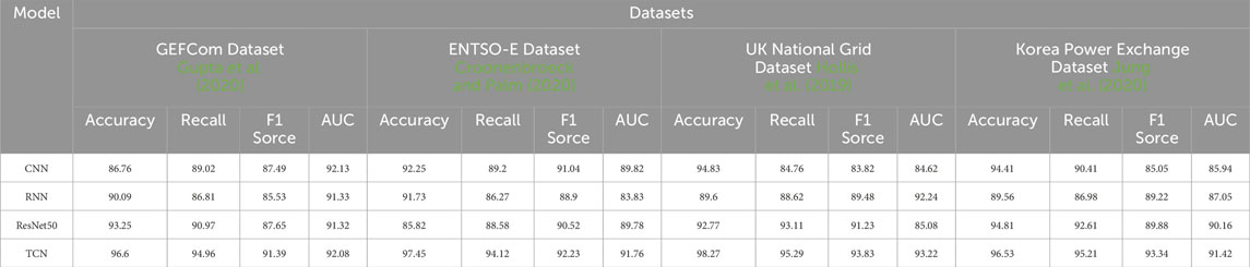
Table 4. Ablation experiment of TCN module.

Figure 7

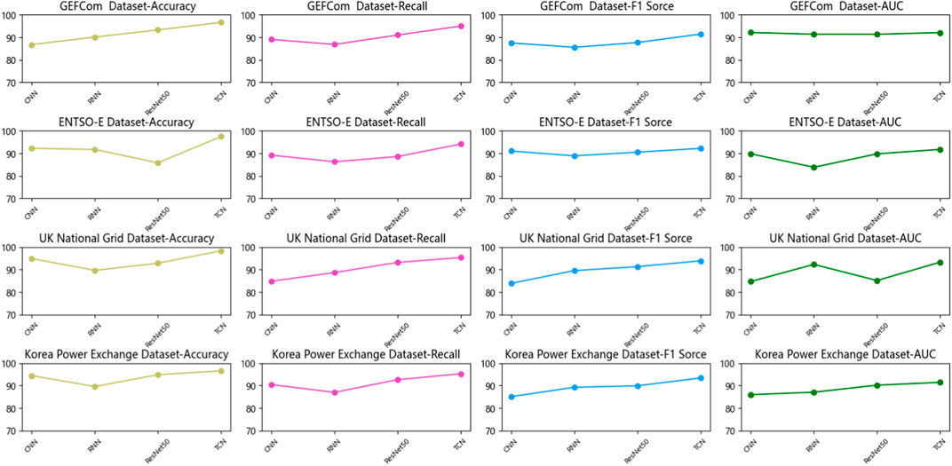
Figure 7. Ablation experiment of TCN module.

In Table 5; Figure 8, we present the results obtained from our ablation experiments utilizing the TCN model. Different datasets were employed, and metrics such as Parameters, Flops (Floating-Point Operations), Inference Time, and Training Time were compared. Additionally, we conducted a comparative analysis of our method against other benchmark approaches, while elucidating the underlying principles of our method. Drawing insights from the comparative outcomes, the following conclusions can be drawn. Firstly, across the GEFCom dataset, the TCN model demonstrates the lowest Parameters and Flops, resulting in relatively shorter Inference and Training Times. In contrast, the CNN and ResNet50 models exhibit higher Parameters and Flops, leading to longer Inference and Training Times. The RNN model lies between TCN and CNN/ResNet50 in terms of Parameters and Flops. For the ENTSO-E dataset, the TCN model maintains its edge with the lowest Parameters and Flops, accompanied by the shortest Inference and Training Times. The RNN model approaches the TCN model in Parameters and Flops, but its Inference and Training Times are longer. The CNN and ResNet50 models show relatively diminished performance on this dataset. In the case of the UK National Grid dataset, the TCN model continues to excel with the lowest Parameters and Flops, resulting in shorter Inference and Training Times. The ResNet50 model’s Parameters and Flops are close to those of the TCN model, but its Inference and Training Times are longer. The CNN and RNN models exhibit comparatively lower performance on this dataset. Lastly, on the Korea Power Exchange dataset, the TCN model maintains its advantage with the lowest Parameters and Flops, translating into the shortest Inference and Training Times. While the ResNet50 and CNN models have Parameters and Flops comparable to the TCN model, their Inference and Training Times are longer. The RNN model performs poorly on this dataset. Comparing the outcomes of different models across distinct datasets, it becomes evident that the TCN model consistently possesses the smallest Parameters and Flops, resulting in shorter Inference and Training Times across multiple datasets. This signifies the TCN model’s efficiency in terms of model architecture and computational attributes, makingx it well-suited for processing time series data. Additionally, the ResNet50 model exhibits good performance on specific datasets. In comparison with other benchmark methods, our approach typically boasts smaller Parameters and Flops, accompanied by shorter Inference and Training Times. Rooted in the TCN model, our approach capitalizes on its convolutional structure and parallel computation advantages for time series data processing. Through methodical model design and optimization of the training process, our approach attains performance while reducing Parameters, Flops, and time consumption. Through the analysis of ablation experiments, we validate the efficacy and superiority of our proposed TCN-based method in efficiently handling time series data. Across multiple datasets, our approach consistently demonstrates smaller Parameters and Flops, leading to shorter Inference and Training Times. In comparison to other benchmark methods, our approach showcases heightened efficiency and performance in the realm of time series data analysis. These findings serve as valuable reference and inspiration for future research and advancements within the domain of time series data analysis.

Table 5

Table 5. Ablation experiment of TCN module.

Figure 8

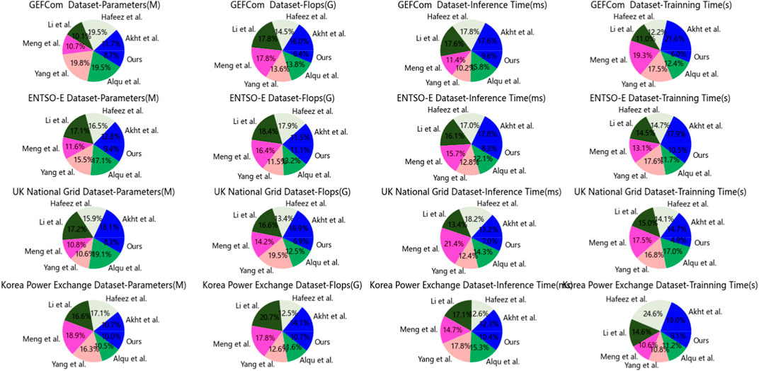
Figure 8. Ablation experiment of TCN module.

4 Summary and discussion

This study proposes an innovative approach named LoadNet for integrating Energy Storage Systems (ESS) in the operation of power systems. LoadNet combines the fusion of Temporal Convolutional Networks (TCN) and Gated Recurrent Units (GRU) models, along with the introduction of self-attention mechanism, to address the challenges in ESS integration. Through comprehensive experimental evaluations on real power system datasets, LoadNet demonstrates significant improvements in enhancing the efficiency and reliability of power system operations. In this study, we utilized multiple power system datasets including GEFCom, ENTSO-E, UK National Grid, and Korea Power Exchange datasets. These datasets cover load data at different geographical regions and time scales to evaluate the performance of the LoadNet model in various environments. Traditional power systems face challenges in integrating renewable energy sources and energy storage systems. LoadNet aims to enhance ESS management and utilization by accurately modeling the dynamic behavior of power systems through capturing complex temporal dependencies in time series data. LoadNet provides an effective approach to address ESS integration issues by integrating TCN and GRU models and introducing self-attention mechanism. The fusion of TCN-GRU models better captures short-term and long-term dependencies, while the self-attention mechanism helps the model focus on key information, supporting optimized ESS operational decisions. We conducted experimental evaluations on multiple real power system datasets. Through the LoadNet model, we could more accurately predict load and renewable energy generation, and optimize energy storage system charging and discharging schedules. Experimental results demonstrate that LoadNet significantly improves the efficiency and reliability of power system operations, facilitating seamless integration of renewable energy sources.

Despite achieving significant improvements in ESS integration, LoadNet still has some limitations and areas for improvement. Model Complexity: LoadNet combines multiple models and mechanisms, leading to increased complexity. Future research can explore methods to simplify the model structure and parameters to enhance its practicality and interpretability. Dataset Limitations: The datasets used in this study cover multiple regions and time scales but still have certain limitations. Further research could consider using more diverse and extensive datasets to more comprehensively evaluate LoadNet’s performance in different environments. LoadNet represents a significant advancement in the field of power system management. Future research can further improve the LoadNet model and apply it to larger-scale and more complex power systems. Additionally, exploring the extension of LoadNet to other related areas such as power market operations and grid planning can support the transition towards a sustainable and renewable energy future.

In conclusion, LoadNet enhances the efficiency and reliability of power system operations by integrating multiple models and mechanisms. Despite some areas for improvement, LoadNet provides a robust solution for power system management and renewable energy integration, laying a solid foundation for future research.

Data availability statement

The original contributions presented in the study are included in the article/Supplementary material, further inquiries can be directed to the corresponding author.

Author contributions

MGL: Conceptualization, methodology, software, validation, formal analysis, investigation, data curation, funding acquisition, writing–original draft. XXH: Conceptualization, validation, formal analysis, visualization, supervision, funding acquisition, writing–review and editing.

Funding

The author(s) declare that no financial support was received for the research, authorship, and/or publication of this article.

Conflict of interest

The authors declare that the research was conducted in the absence of any commercial or financial relationships that could be construed as a potential conflict of interest.

Publisher’s note

All claims expressed in this article are solely those of the authors and do not necessarily represent those of their affiliated organizations, or those of the publisher, the editors and the reviewers. Any product that may be evaluated in this article, or claim that may be made by its manufacturer, is not guaranteed or endorsed by the publisher.

References

Akhtaruzzaman, M., Hasan, M. K., Kabir, S. R., Abdullah, S. N. H. S., Sadeq, M. J., and Hossain, E. (2020). Hsic bottleneck based distributed deep learning model for load forecasting in smart grid with a comprehensive survey. IEEE Access 8, 222977–223008. doi:10.1109/access.2020.3040083

CrossRef Full Text | Google Scholar

Alquthami, T., Zulfiqar, M., Kamran, M., Milyani, A. H., and Rasheed, M. B. (2022). A performance comparison of machine learning algorithms for load forecasting in smart grid. IEEE Access 10, 48419–48433. doi:10.1109/access.2022.3171270

CrossRef Full Text | Google Scholar

Copiaco, A., Himeur, Y., Amira, A., Mansoor, W., Fadli, F., Atalla, S., et al. (2023). An innovative deep anomaly detection of building energy consumption using energy time-series images. Eng. Appl. Artif. Intell. 119, 105775. doi:10.1016/j.engappai.2022.105775

CrossRef Full Text | Google Scholar

Croonenbroeck, C., and Palm, M. (2020). A spatio-temporal durbin fixed effects iv-model for entso-e electricity flows analysis. Renew. Energy 148, 205–213. doi:10.1016/j.renene.2019.11.133

CrossRef Full Text | Google Scholar

Geng, G., He, Y., Zhang, J., Qin, T., and Yang, B. (2023). Short-term power load forecasting based on pso-optimized vmd-tcn-attention mechanism. Energies 16, 4616. doi:10.3390/en16124616

CrossRef Full Text | Google Scholar

Gupta, P., Malsa, N., Saxena, N., Agarwal, S., and Singh, S. P. (2020). “Short-term load forecasting using parametric and non-parametric approaches,” in Soft computing: theories and applications: proceedings of SoCTA 2018 (Germany: Springer), 747–755.

CrossRef Full Text | Google Scholar

Hafeez, G., Alimgeer, K. S., and Khan, I. (2020a). Electric load forecasting based on deep learning and optimized by heuristic algorithm in smart grid. Appl. Energy 269, 114915. doi:10.1016/j.apenergy.2020.114915

CrossRef Full Text | Google Scholar

Hafeez, G., Khan, I., Jan, S., Shah, I. A., Khan, F. A., and Derhab, A. (2021). A novel hybrid load forecasting framework with intelligent feature engineering and optimization algorithm in smart grid. Appl. Energy 299, 117178. doi:10.1016/j.apenergy.2021.117178

CrossRef Full Text | Google Scholar

Han, Z., Lu, Y., Li, Y., Wu, R., and Huang, Z. (2022). Strategy to combine two functional components: efficient nano material development for iodine immobilization. Chemosphere 309, 136477. doi:10.1016/j.chemosphere.2022.136477

PubMed Abstract | CrossRef Full Text | Google Scholar

Haque, A., and Rahman, S. (2022). Short-term electrical load forecasting through heuristic configuration of regularized deep neural network. Appl. Soft Comput. 122, 108877. doi:10.1016/j.asoc.2022.108877

CrossRef Full Text | Google Scholar

Himeur, Y., Alsalemi, A., Bensaali, F., and Amira, A. (2020). A novel approach for detecting anomalous energy consumption based on micro-moments and deep neural networks. Cogn. Comput. 12, 1381–1401. doi:10.1007/s12559-020-09764-y

CrossRef Full Text | Google Scholar

Himeur, Y., Alsalemi, A., Bensaali, F., and Amira, A. (2021a). Smart power consumption abnormality detection in buildings using micromoments and improved k-nearest neighbors. Int. J. Intelligent Syst. 36, 2865–2894. doi:10.1002/int.22404

CrossRef Full Text | Google Scholar

Himeur, Y., Ghanem, K., Alsalemi, A., Bensaali, F., and Amira, A. (2021b). Artificial intelligence based anomaly detection of energy consumption in buildings: a review, current trends and new perspectives. Appl. Energy 287, 116601. doi:10.1016/j.apenergy.2021.116601

CrossRef Full Text | Google Scholar

Hollis, D., McCarthy, M., Kendon, M., Legg, T., and Simpson, I. (2019). Haduk-grid—a new UK dataset of gridded climate observations. Geoscience Data J. 6, 151–159. doi:10.1002/gdj3.78

CrossRef Full Text | Google Scholar

Jung, Y., Jung, J., Kim, B., and Han, S. (2020). Long short-term memory recurrent neural network for modeling temporal patterns in long-term power forecasting for solar pv facilities: case study of South Korea. J. Clean. Prod. 250, 119476. doi:10.1016/j.jclepro.2019.119476

CrossRef Full Text | Google Scholar

Karthik, S. S., and Kavithamani, A. (2021). Oelf: short term load forecasting for an optimal electrical load forecasting using hybrid whale optimization based convolutional neural network. J. Ambient Intell. Humaniz. Comput. 14, 7023–7031. doi:10.1007/s12652-021-03556-4

CrossRef Full Text | Google Scholar

Khan, Z. A., Hussain, T., Ullah, W., and Baik, S. W. (2023). A trapezoid attention mechanism for power generation and consumption forecasting. IEEE Trans. Industrial Inf., 1–13. doi:10.1109/tii.2023.3335453

CrossRef Full Text | Google Scholar

Khan, Z. A., Khan, S. A., Hussain, T., and Baik, S. W. (2024). Dspm: dual sequence prediction model for efficient energy management in micro-grid. Appl. Energy 356, 122339. doi:10.1016/j.apenergy.2023.122339

CrossRef Full Text | Google Scholar

Li, J., Deng, D., Zhao, J., Cai, D., Hu, W., Zhang, M., et al. (2020a). A novel hybrid short-term load forecasting method of smart grid using mlr and lstm neural network. IEEE Trans. Industrial Inf. 17, 2443–2452. doi:10.1109/tii.2020.3000184

CrossRef Full Text | Google Scholar

Li, Z., Huang, Z., Guo, L., Shan, L., Yu, G., Chong, Z., et al. (2023). Cognitive knowledge graph generation for grid fault handling based on attention mechanism combined with multi-modal factor fusion. Comput. Electr. Eng. 111, 108855. doi:10.1016/j.compeleceng.2023.108855

CrossRef Full Text | Google Scholar

Lin, Z., and Xu, F. (2023). “Simulation of robot automatic control model based on artificial intelligence algorithm,” in 2023 2nd International Conference on Artificial Intelligence and Autonomous Robot Systems (AIARS) (IEEE), USA, 29-31 July 2023 (IEEE), 535–539.

CrossRef Full Text | Google Scholar

Ma, J., Teng, Z., Tang, Q., Guo, Z., Kang, L., Wang, Q., et al. (2023). A novel multi-source feature fusion framework for measurement error prediction of smart electricity meters. IEEE Sensors J. 23, 19571–19581. doi:10.1109/jsen.2023.3292347

CrossRef Full Text | Google Scholar

Meng, F., and Wang, X. (2023). Digital twin for intelligent probabilistic short term load forecasting in solar based smart grids using shark algorithm. Sol. Energy 262, 111870. doi:10.1016/j.solener.2023.111870

CrossRef Full Text | Google Scholar

Peng, Q., and Liu, Z.-W. (2020). “Short-term residential load forecasting based on smart meter data using temporal convolutional networks,” in 2020 39th Chinese Control Conference (CCC), New York, 27-29 July 2020 (IEEE), 5423–5428.

CrossRef Full Text | Google Scholar

Shaqour, A., Ono, T., Hagishima, A., and Farzaneh, H. (2022). Electrical demand aggregation effects on the performance of deep learning-based short-term load forecasting of a residential building. Energy AI 8, 100141. doi:10.1016/j.egyai.2022.100141

CrossRef Full Text | Google Scholar

Shi, H., Wang, L., Scherer, R., Woźniak, M., Zhang, P., and Wei, W. (2021). Short-term load forecasting based on adabelief optimized temporal convolutional network and gated recurrent unit hybrid neural network. IEEE Access 9, 66965–66981. doi:10.1109/access.2021.3076313

CrossRef Full Text | Google Scholar

Wang, C., Wang, Y., Ding, Z., and Zhang, K. (2023a). Probabilistic multi-energy load forecasting for integrated energy system based on bayesian transformer network. IEEE Trans. Smart Grid 15, 1495–1508. doi:10.1109/tsg.2023.3296647

CrossRef Full Text | Google Scholar

Wang, J., Han, L., Zhang, X., Wang, Y., and Zhang, S. (2023b). Electrical load forecasting based on variable t-distribution and dual attention mechanism. Energy 283, 128569. doi:10.1016/j.energy.2023.128569

CrossRef Full Text | Google Scholar

Wu, R., Han, Z., Chen, H., Cao, G., Shen, T., Cheng, X., et al. (2021). Magnesium-functionalized ferro metal–carbon nanocomposite (mg-femec) for efficient uranium extraction from natural seawater. ACS ES&T Water 1, 980–990. doi:10.1021/acsestwater.0c00262

CrossRef Full Text | Google Scholar

Wu, Y., Sheng, Y., Guo, N., Li, F., Tian, Y., and Su, X. (2022). “Hybrid deep network based multi-source sensing data fusion for fdia detection in smart grid,” in 2022 Asia Power and Electrical Technology Conference (APET), China, November 11-13, 2022 (IEEE), 310–315.

CrossRef Full Text | Google Scholar

Yang, Y., Li, W., Gulliver, T. A., and Li, S. (2019). Bayesian deep learning-based probabilistic load forecasting in smart grids. IEEE Trans. Industrial Inf. 16, 4703–4713. doi:10.1109/tii.2019.2942353

CrossRef Full Text | Google Scholar

Yanmei, J., Mingsheng, L., Yangyang, L., Yaping, L., Jingyun, Z., Yifeng, L., et al. (2023). Enhanced neighborhood node graph neural networks for load forecasting in smart grid. Int. J. Mach. Learn. Cybern. 15, 129–148. doi:10.1007/s13042-023-01796-8

CrossRef Full Text | Google Scholar

Yi, S., Liu, H., Chen, T., Zhang, J., and Fan, Y. (2023). A deep lstm-cnn based on self-attention mechanism with input data reduction for short-term load forecasting. IET Generation, Transm. Distribution 17, 1538–1552. doi:10.1049/gtd2.12763

CrossRef Full Text | Google Scholar

Zhang, K., Li, H., Cao, S., Lv, S., Yang, C., and Xiang, W. (2023). Trusted multi-source information fusion for fault diagnosis of electromechanical system with modified graph convolution network. Adv. Eng. Inf. 57, 102088. doi:10.1016/j.aei.2023.102088

CrossRef Full Text | Google Scholar

Zhou, F., Zhou, H., Li, Z., and Zhao, K. (2022). Multi-step ahead short-term electricity load forecasting using vmd-tcn and error correction strategy. Energies 15, 5375. doi:10.3390/en15155375

CrossRef Full Text | Google Scholar