 Wenhu Tang
 Tong Qian
- School of Electric Power Engineering, South China University of Technology, Guangzhou, China
The accuracy of photovoltaic (PV) power forecasting techniques relies not only on high-quality spatiotemporal data but also on an efficient feature-mining methodology. In this study, a spatiotemporal power forecasting model based on the broad learning system (BLS) and the improved backtracking search optimization algorithm (IBSOA) is proposed. The objective is to enhance the accuracy of PV power predictions while reducing the time-intensive training process associated with an extensive set of broad learning system parameters. The spatiotemporal attributes of historical data from multiple PV sites are clustered using a self-organizing map. The clustering analysis explores the spatiotemporal correlation among five photovoltaic (PV) power stations for each season between 2017 and 2018. Subsequently, the IBSOA is employed to optimize the hyperparameters of the BLS model, particularly the mapping and enhancement nodes. By utilizing hyperparameter optimization, a BSOA-based broad learning model is introduced to achieve superior accuracy. The results are assessed using the proposed method in comparison with three popular optimization algorithms: 1) genetic algorithm (GA), 2) bird swarm algorithm (BSA), and 3) backtracking search optimization algorithm (BSOA). All scenarios are validated and compared using PV plant data from the DKA center in Australia. The root-mean-square error (RMSE) indicators of the proposed prediction method are consistently lower than the worst-case scenario in each season, decreasing by 3.2283 kW in spring, 3.9159 kW in summer, 1.3425 kW in autumn, and 1.4058 kW in winter. Similarly, the mean absolute percentage error (MAPE) exhibits a reduction compared to the worst case, with a decreases of 0.882% in spring, 1.2399% in summer, 1.803% in autumn, and 1.087% in winter. The comprehensive results affirm that the proposed method surpasses alternative optimization techniques, delivering high-quality power forecasts for the given case study.
1 Introduction
In light of their potential environmental and economic benefits, renewable energy sources have garnered considerable attention for their projected influence on the future of power grids (Qian et al., 2020). These sources offer the potential to enhance voltage profiles and power supply quality for both energy suppliers and consumers (Li et al., 2023a), thereby contributing to reduced power losses, decreased pollution, and cost savings in specific scenarios. Within the array of energy sources, the assimilation of photovoltaic (PV) power generation into conventional power grids poses inherent stability challenges. This is mainly attributed to the intermittent characteristics of renewable energy sources and the variability introduced by meteorological factors (Hu et al., 2020). Even though meteorological and environmental elements impact photovoltaic (PV) output, resulting in noteworthy fluctuations, the extensive integration of PV brings forth considerable security challenges to the power grid system (Li et al., 2023b). In such contexts, precise PV power forecasting becomes indispensable not only for ensuring the reliable and stable utilization of renewable energy sources but also for minimizing the demand for additional balancing energy and reserve power to accommodate other forms of power generation.
The accuracy of photovoltaic (PV) power forecasting is influenced by a multitude of factors, adding intricacy to the prediction process. These factors encompass the forecasting horizon (Khuntia et al., 2016), the selection of inputs in the forecasting model (Ghofrani et al., 2015), and performance assessment (Choi et al., 2021). To enhance accuracy, it is crucial to undertake correlation analysis optimization (Li et al., 2015) and employ uncertainty estimation and approximations (Zhou et al., 2020). These processes map relationships between the input and output through historical parameter estimation in the development of PV power forecasting approaches. The accuracy of these models is intricately tied to both the quantity and quality of data, necessitating extensive datasets and meticulous data preprocessing (Rahman et al., 2023). By integrating deep learning, heuristic algorithms, and innovative frameworks (Hafeez et al., 2020a), the refined approaches not only improve accuracy but also tackle challenges related to stability and convergence rate, contributing to the dynamic evolution of smart grid technologies (Hafeez et al., 2020b). In recent years, deep neural networks (DNNs) have emerged as a viable option for PV power forecasting despite their limited nonlinear mapping capabilities. An advantage of using DNNs lies in their capacity to simplify high-dimensional and nonlinear problems in contrast to physical methods (Yildiz et al., 2021) that are well-suited for stable conditions. Hossain and Mahmood (2020) proposed a LSTM (long short-term memory) neural network with the synthetic irradiance forecast and algorithm, whichachieves over 30% accuracy improvement in PV power forecasting. Based on LSTM, with a focus on accuracy, Aslam et al. (2021) employed the Bayesian optimization algorithm in conjunction with LSTM for power forecasting, thereby demonstrating its efficiency. Shaqour et al. (2022) proposed a DNN combined with the bi-directional gated recurrent unit with fully connected layers (Bi-GRU-FCL), which achieves faster training time and fewer learnable parameters based on five aggregation levels based on a dataset in Japan. Lin et al. (2020) introduced an enhanced moth–flame optimization algorithm and applied it to optimize the support vector machine (SVM). The results demonstrated the strong performance of the model on both sunny and rainy days. Fekri et al. (2021) proposed an adaptive recurrent neural network (ARNN) prediction model for online learning. The model dynamically adjusts its hyperparameters in response to new data, allowing the prediction process to adapt to changing conditions. A comparative analysis of the integrating feature engineering (FE) and a modified fire-fly optimization (mFFO) algorithm with support vector regression (SVR) against benchmark frameworks highlights the superior performance in terms of accuracy, stability, and convergence rate (Hafeez et al., 2021). In summary, the above studies contribute to the evolving landscape of PV power and load forecasting, showcasing diverse approaches and improvements in accuracy through the integration of deep learning techniques and optimization algorithms.
Building upon the aforementioned studies, it has been demonstrated that employing appropriate optimization methods for DNNs can result in enhanced prediction accuracy, leading to improved forecasting outcomes. Addressing the inherent non-linear characteristics of data (Kleissl, 2013), research efforts have explored intelligent algorithms that do not rely on predefined mathematical models. Oudjana et al. (2013) and Konjić et al. (2015) conducted a comparative study involving an artificial neural network (ANN) model for PV output forecasting against three conventional mathematical approaches and regression models. The findings underscored the significantly superior forecast accuracy achieved by the ANN. Although each approach has its merits and limitations, genetic algorithm (GA)-based optimization emerges as the most popular and effective technique for optimizing weights and inputs in forecasting models (Ding et al., 2011), particularly when used in conjunction with an ANN (Deniz et al., 2016). Pedro and Coimbra (2012) reported enhancements in their ANN-based PV power forecasting model through GA optimization, resulting in improved forecast accuracy. In comparison to GA, GA-based optimization demonstrates easier convergence and requires fewer parameter adjustments (Viet et al., 2020). At present, particle swarm optimization (PSO) is widely used in function optimization, according to Ahmed et al. (2020), neural network training and parameter selection, fuzzy system control, and other applications as a substitute for GA. Nevertheless, mainstream optimization algorithms such as GA and PSO often display an increased vulnerability to getting ensnared in local extrema (Bamdad et al., 2017). The optimization direction is contingent upon parameter settings, thereby impacting the time and cost of optimization. Although the convolution operation can meet the requirements and yield a satisfactory performance, it introduces potential issues. The local influence of the convolution kernel poses a risk of introducing false information, and data transformation contributes to an escalation in the complexity of the prediction model.
Furthermore, traditional neural network prediction methods typically employ multiple hidden layers to construct forecasting models. Although these models efficiently learn and extract valuable features from input data, they are characterized by shallow architectures and limited capabilities in representing complex nonlinear functions. As a result, these models have a tendency to underfit complex prediction tasks, resulting in a decline in accuracy, particularly when dealing with large-scale data-driven problems. In contrast to DNNs, the broad learning system (BLS), as an alternative method, enhances the generalization performance by expanding the width of a single hidden layer rather than improving its approximation capabilities through the extension of deep architectures (Feng et al., 2022). Some researchers utilize BLS as a method to enhance the accuracy of forecasting when dealing with large-scale datasets (Chen and Liu, 2017; Cheng et al., 2022; Zhu et al., 2022). The expanded broad structure of BLS ensures its strong approximation capability of nonlinear mapping (Wang et al., 2020) to ensure the accuracy of prediction results while significantly reducing computational costs, and the accuracy can be maintained using proper optimization techniques (Gong et al., 2022).
It is crucial to note that the effectiveness of certain methodology comparisons may be compromised because various prediction models are included in the comparison sections, each employing different hyperparameter tuning approaches and distinct hyperparameter configurations. To uphold the effectiveness of the comparison results, the research concentrates on tuning hyperparameters within the same forecasting model while allowing for adjustability in the algorithms. In the present research, the BLS model is employed as a framework for short-term PV power forecasting. The self-organizing map (SOM) is introduced to evaluate the spatiotemporal correlations of five PV stations. The backtracking search optimization algorithm (BSOA) examined in this study demonstrated effectiveness in addressing engineering optimization problems (Civicioglu, 2013), given that the initialization step does not demand specific tuning. However, BSOA is not without drawbacks as it requires substantial information in the evolution process to regulate a correct optimization search direction. Moreover, ensuring the population diversity poses challenges, potentially resulting in convergence on the local optima. Consequently, the subsequent sections detail improvements aimed at addressing the limitations of BSOA. An improved backtracking search optimization algorithm (IBSOA) is employed to tune the hyperparameters of BLS. The improved backtracking search algorithm-based broad learning system (IBSOA-BLS) method is compared to other meta-heuristic algorithm variants, including genetic algorithm-based learning system (GA-BLS), backtracking search algorithm-based learning system (BSOA-BLS), and bird swarm algorithm-based learning system (BSA-BLS), to demonstrate its superior prediction accuracy.
Thus, the contribution of this paper includes the following:
• Employment of the BLS to predict PV power generation, which is a computationally efficient method that consistently delivers high forecasting accuracy compared to other neural network-based prediction approaches.
• Evaluation of PV power spatiotemporal correlation is conducted through a copula-based self-organizing map to investigate the inner characteristics among the five PV stations.
• To enhance accuracy, the BSOA algorithm is improved by addressing the selection and mutation processes to mitigate the random optimization search problem.
• The comparison involves the BLS power forecasting model tuned by the improved algorithm and other metaheuristic algorithms, specifically GA, BSA, and BSOA.
The remaining sections of the paper are organized as follows: Section 2 initiates with the definition of the broad learning system. Section 3 introduces the enhancements to the backtracking search optimization algorithm and evaluates the performance of IBSOA. Section 4 outlines the IBSOA-BLS prediction model, covering data preprocessing and clustering. Section 5 delves into the power forecasting results using the proposed method and conducts comparisons. Lastly, Section 6 concludes the paper.
2 Broad learning system
Random vector link neural networks (RVFLNNs) serve as the foundation of BLS. BLS operates by extracting features from the input data through feature mapping, subsequently transforming these feature nodes into enhancement nodes using nonlinear transformations, which further employs an incremental learning method to update the output weights of these enhanced nodes. The approach differs from traditional RVFLNN, where input data are directly accepted and enhancement nodes are established. In deep learning networks, improved fitting capabilities result from the addition of extra network layers rather than simply increasing the number of nodes. Based on RVFLNN, BLS training facilitates swift updates and refinements to the prediction system, contrasting with deep neural networks, where learning time progresses monotonically. By extending the feature and enhancement nodes, BLS improves the network performance and model fitting capabilities. The system consists of three fundamental components: 1) mapping feature nodes, 2) enhancement nodes, and 3) an output matrix as shown in Figure 1.
BLS training comprises two primary phases: first, the weights for the mapping and enhancement nodes are randomly generated, and second, the weights between the hidden layer and the output layer are calculated. In simpler terms, during training, the sole weight that requires acquisition is the one connecting the final output layer to the hidden layer as the weights of the BLS random layer are generated randomly. In the initial stage, BLS forwards the original input data as mapping features, following which the structure can be expanded using the enhancement nodes. The random feature mapping stage distinguishes BLS from other established learning techniques, such as the single-layer feedforward network (SLFN), which updates its parameters through gradient descent, and the support vector machine (SVM), which utilizes kernel functions for feature mapping. The mapping feature nodes can be represented as follows:
where X is the input data and Wf and βf are the weighting matrix and bias of feature nodes, respectively. Via the sparse autoencoder (Yang et al., 2021), BLS uses the mapping function ϕ to extend the enhancement nodes. The mth group of the nodes can be expressed as follows:
where ζ is the nonlinear transformation function and We and βe are the weight matrix and bias of enhancement nodes, respectively. Then, the output of BLS can be obtained from the following equation:
where
Numerous researchers have enhanced the generation of random mapping feature nodes to align with diverse industrial requirements. Empirical experiments have shown that diverse activation functions enable the model to acquire a range of nonlinear expression capabilities. The commonly used transformation functions are listed in Table 1 and the Gaussian function is used for the enhancement node calculation in this research.
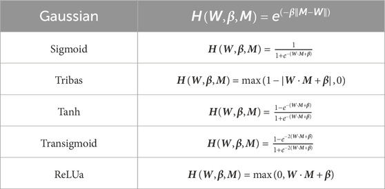
Table 1. Transformation function for generating enhancement nodes.
3 Improvement of the backtracking search optimization algorithm
3.1 Backtracking search optimization algorithm
The backtracking search optimization algorithm, also referred to as BSA or BSOA, is not sensitive to the initializations of population, so initialization can be generated randomly. Theoretically, the BSOA usually follows the following five steps (Hassan and Rashid, 2020):
• Initialize two populations popi,j and
where popi,j and
• Population selection I: the historical population is updated by equation (6) with the uniform distribution from the previous population selection. αs1 and αs2 represent that the selection process happens randomly. Then, a permut function is used in equation (7) to change the order of each element in the old population set.
• Mutation: the process generates the initial form of the historical data-based trial population by using two significant populations popi,j and
where F is the population step change and is defined as 3 × snd and snd is the standard normal distribution in the numerical range of 0 to 1. It controls the search direction of the matrix
• Crossover: the crossover process is as shown in equation (9). The process is divided into two steps. In the first step, an N × D mapping mi,j matrix is generated and initialized. The matrix is updated by means of two strategies with a ceiling function and a random integer function randi. αs1 < αs2 represents a probabilistic condition to indicate its randomness. Second, the crossover population is mapped with popi,j or popmut according to equations (10) and (11). It should be noted that equations (10) and (11) are only applied for equation (9). At the end of the crossover process, if the population generated from equation (9) overflows the lower or upper boundary, the population is reproduced via equation (12).
Here, R is a re-scale factor of reproduction selected between 0 and 1,
• Population selection II: in this stage, based on a greedy selection mechanism, popi,j that has better fitness values is used to update the new population
BSOA proves effective for solving engineering optimization problems as the initialization step does not require specific tuning. Nevertheless, BSOA has drawbacks since it necessitates sufficient information in the evolution process to control a correct optimization search direction. Additionally, ensuring population diversity is challenging, potentially leading to a convergence on the local optima.
3.2 Data mining BSOA with a mutual learning method
To address the limitations of BSOA, which does not consider historical references and the representation of the characteristics of extensive data, the research utilizes a winner tendency-based method to improve BSOA performance. The basic idea of topological opposition-based learning is to find the feasible solution from an opposite direction of the search space. By evaluating the two solutions (4) and (5) at the same time, it provides a faster searching speed for the best solution. The learning operator and the improved mutation operator are used to inspect the best individual/solution in each generation and drive the current population to approach it. Unlike BSOA, the improvement also records the best and mean fitness of all individuals in each iteration and uses them for next-generation optimization.
Topological opposition-based learning operator (TOLO) is featured by its learning behavior from the best fitness in each generation. The learning operator is developed based on the opposition point operator, as defined in equation (14):
It is noted that popi = [popi1, popi2, …, popij, …, popiD], popi,j ∈ [lbj, ubj], and i and j are the sample size and dimension, respectively. Second, based on the initialization of population in BSOA, the TOLO updates the population by measuring the distance of the best fitness and the current population and expresses it as in equation (15).
where popopt,j is the best population at the jth dimension.
Improved mutation operator: unlike in BSOA, the information about an individual in the mutation process is updated with other historical and present data. The improved mutation operator executes a procedure to mutate the present individuals by taking the optimum and mean individuals in each iteration into consideration.
where α1 and α2 are random numbers between 0 and 1, popm is the mean individual in a population, and F is the control parameter defined in BSOA.
3.3 IBSOA performance evaluation
To evaluate the effectiveness of the proposed IBSOA, an investigation was undertaken utilizing eight benchmark functions, each featuring two- to twenty-dimensional inputs. Links to these eight functions have been included in Appendix A. The eight benchmark functions utilized in this study represent widely employed functions and datasets for testing forecasting scenarios. Their differentiation is grounded in similarities in physical properties, datasets, and shapes. These testing functions serve the purpose of parametric optimization and are featured as representative examples of engineering problems. The test benches used for the evaluation of each algorithm are presented in Table 2 and the results are shown in Table 3, where f1 to f4 exhibit multiple local minima and a singular global minimum, rendering them more representative of typical engineering functions. f5 is evaluated on the cube shape and has asymptotic characteristics. f6 is evaluated on the hypercube and is designed for regression problems. f7 exhibits a high curvature in certain variables and a lower curvature in others. The presence of interactions and nonlinear effects make f8 particularly challenging in convergence.
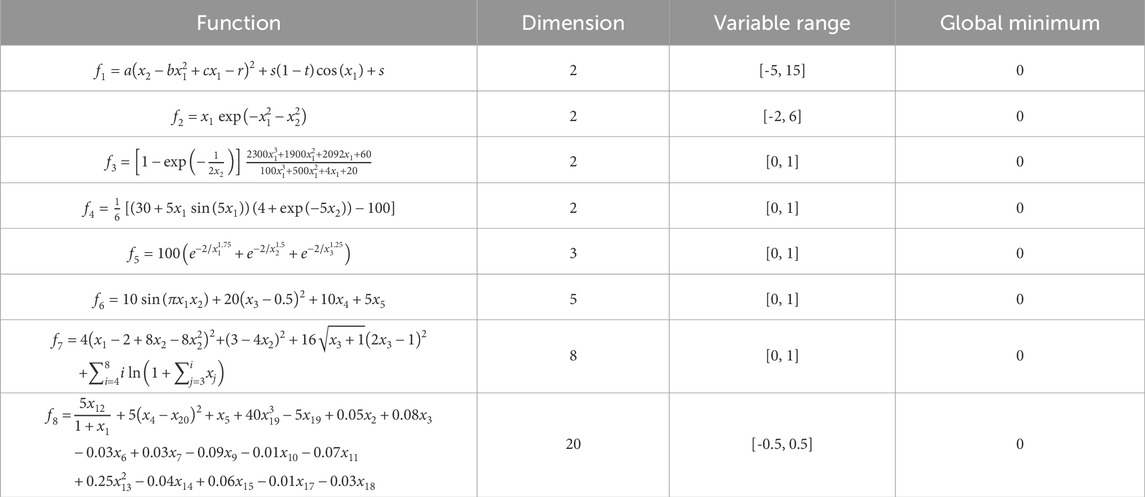
Table 2. Test functions.
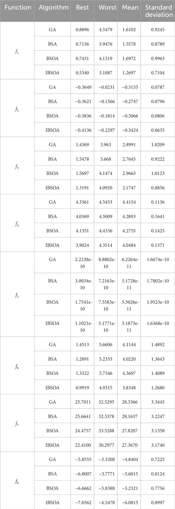
Table 3. Test function results.
The overall performance from Table 3 shows that the convergence ability of IBSOA is better than the other algorithms when dealing with multiple local minima, asymptotic characteristics, and regression problems. In function, defects in the evaluation become apparent as slight changes in variables result in significant alterations in the function output, indicating a high curvature. In function f7, deficiencies in the evaluation become evident as minor changes in variables lead to substantial alterations in the function output, indicative of a high curvature. The increased sensitivity poses a challenge to the performance of the improved algorithm. The nonlinear effects of function f8 also impact the standard deviation but still yield the best fitness compared to other algorithms.
4 PV power forecasting based on IBSOA-BLS
4.1 Model fitness
In order to optimize the hyperparameters of BLS, they are denoted as x1, x2, and x3, while the learning rate is represented by η in the fitness function. To elaborate, x1 corresponds to the mapping feature nodes, x2 pertains to the enhancement nodes, and x3 relates to the winner neuron nodes. When the population in the IBSOA algorithm is coded, each individual is a vector X (x1, x2, x3, η), and the optimization problem of the model parameter can be expressed as follows:
where N is the number of samples and yi and Yi are the predicted and true power values of the ith sample, respectively. The main objective of the proposed method is to optimize the fitness function, and the process of optimization is listed below and displayed in Figure 2.
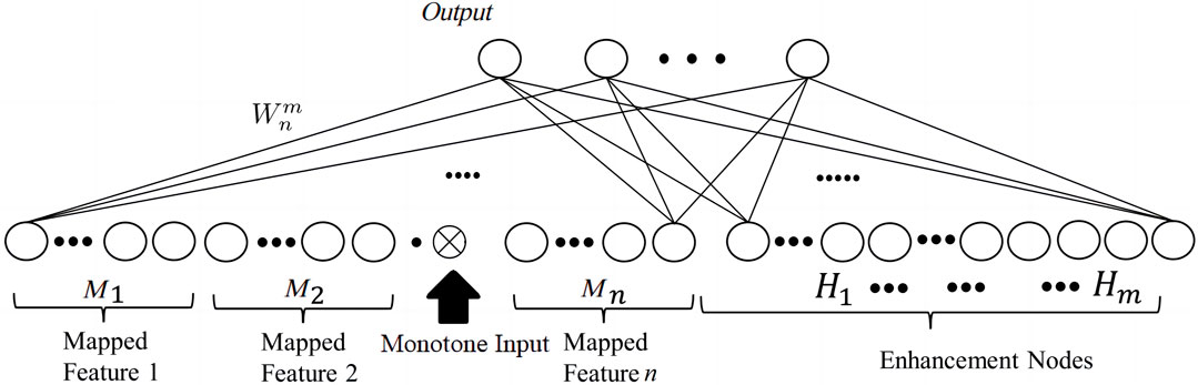
Figure 1. BLS topology.
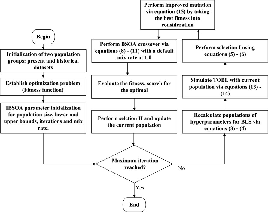
Figure 2. IBSOA optimization flowchart.
Step 1. The data from the DKA PV power station have singular value queries, and some are missing. To handle the missing data, the data from past years (2014–2016) are considered for data imputation.
Step 2. The self-organizing map method (Hu et al., 2019) is employed to identify meteorological factors that exhibit strong correlations with PV power and eliminate redundant meteorological factors.
Step 3. The comprehensive similarity index is utilized to choose the historical date that closely resembles the predicted date.
Step 4. The parameters, including the number of hidden layers, training iterations, IBSOA population size, and training cycles for the BLS model, are initialized. The IBSOA algorithm is employed to tune hyperparameters.
Step 5. The IBSOA-BLS network structure is initially pre-trained and subsequently fine-tuned in a reverse order. The training and testing datasets are then utilized to generate forecasts for PV power output.
4.2 Dataset preprocessing
The dataset obtained from the Alice Springs station at the DKA solar power center in Australia includes PV power generation and the corresponding meteorological measurements. The five PV stations operate with rated capacities of 226.8 kW, 22.6 kW, 38.3 kW, 327.6 kW, and 105.9 kW, respectively. The data span from 1 March 2017 to 1 March 2018, and the resolution is at 5-min intervals. The IZBSOA-BLS proposed in this paper aims to predict intra-hour power outputs from 5 minutes to 1 hour ahead.
As the PV power output is zero during nighttime, the predictive analysis focuses on the time period from 07:00 to 18:00 on the forecasted day. In a single day, there are a total of 127 data sampling points. Following the methodology described in the preceding section for identifying analogous days, five historical days similar to the forecasted period are selected as training instances. Subsequently, the model performance is evaluated by testing it on the 127 power values associated with the predicted days. In light of the analysis results regarding the factors impacting PV power, the input variables for the predictive model are defined as follows: PV power generation on analogous days, global radiation, and diffuse radiation. Due to the similarity in the spatiotemporal correlation of PV power characteristics, as indicated in Figures 3 and 4, only the results for the 226.8 kW PV station are presented. Table 4 contains the data on power forecasting. During the data cleansing process, linear interpolation and historical data (2014–2016) are applied and considered to compensate for the missing parts in the 2017–2018 dataset. Consequently, 21 days at the end of each season are used as testing data, while the remainder is designated as training data. The input variables for prediction models encompass PV power, as well as temperature, wind speed, and solar irradiance. The self-organizing map (SOM) is an artificial neural network inspired by biological models of neural systems from the 1970s (Barreto, 2007). It functions as a neural network-based dimensionality reduction algorithm, utilizing an unsupervised learning approach. SOM is commonly used to represent a high-dimensional dataset as a two-dimensional discretized pattern, simplifying complex problems for easier interpretation. The employment of SOM achieves dimensionality reduction while preserving the topological relationships present in the original feature space (Kohonen, 2013). SOM clusters the spatial dependence of the PV power dataset into multiple subsets, each corresponding to their individual external conditions. The clustered data include PV power, wind speed, temperature, global radiation, and diffused radiation. Subsequently, the spatio-temporal dependence of PV power is derived from the historical PV power data within each subset.
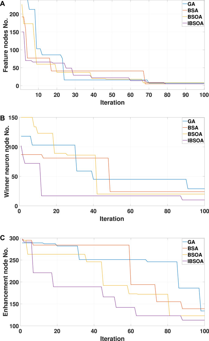
Figure 3. Hyperparameter optimization of BLS using various algorithms during the spring season: (A) Feature node optimization, (B) Winner neuron node optimization, (C) Enhancement node optimization.
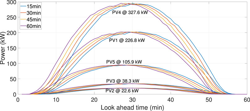
Figure 4. PV plants clustering in Spring.
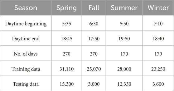
Table 4. PV forecasting dataset.
In this research, PV spatio-temporal correlation clustering for two seasons, spring and summer, is illustrated in Figures 3 and 4. The clustering process in this research and more clustering results in other seasons are verified and evaluated by Zhou et al. (2022). The time granularity is set to 15 min instead of 5 min due to the time-consuming process of SOM clustering during MATLAB simulation. The results of Figures 3 and 4 demonstrate that PV samples belonging to the same cluster display analogous PV power patterns, signifying congruent spatio-temporal correlations. Thus, due to similar PV power characteristics, one PV station (226.8 kW capacity) is used for model forecasting in the following analysis.
5 Analysis of results and discussion
In this research, only sunny days are considered. The results are shown in the manner of four seasons. Each season begins at 5:35 in spring, 5:50 in summer, 6:30 in autumn, and 7:10 in winter. The daytime ends at 18:45 in spring, 19:50 in summer, 17:50 in autumn, and 18:40 in winter. The algorithms are executed 10 times, and the average is taken to ensure validity; the mean values are used for evaluation. The measured values and prediction of PV power in different seasons are shown in Figures 5 and 6. The computational efficiency of the algorithm-based BLS is shown in Table 5. The simulation results are implemented and completed via MATLAB R2023a on a PC with Intel Core i7-7700 CPU @ 3.4 GHz and 16 GB RAM. The configurations of the four algorithms are shown in Table 6. The hyperparameter optimization processes of BLS in spring are illustrated in Figure 7. The optimization performance of IBSOA yields better outcomes when searching for the best fitness within 100 iterations. This is attributed to the enhancement of BSOA, which incorporates historical data (mean and the best fitness in each iteration) during the selection and mutation processes to regulate the correct optimization search direction and maintain dynamic population diversity. The enhancement also improves the accuracy of the forecasting model by obtaining optimized hyperparameters for the given iteration through the enhanced search ability of BSOA. The forecasting results illustrate that the prediction deviations of each model are more significant during the period from 20 to 40 min compared to the deviations from 12:00 to 18:00 during sunny periods. The phenomenon can be attributed to the movement of clouds in the early morning, which impacts the electricity generation at the PV power station, leading to increased power fluctuations and, thus, making prediction more challenging. Notably, the proposed IBSOA-BLS exhibits superior predictive performance compared to the other three models, while GA, BSA, and IBSOA also demonstrate relatively better predictive capabilities. To provide an accurate assessment of the prediction performance of the four algorithms, the mean square error (MSE), the root-mean-square error (RMSE), the mean absolute error (MAE), and the mean absolute percentage error (MAPE) are employed for a thorough analysis of each model’s prediction effectiveness.
where N is the sample number, x is the measured value of power, and x′ is the prediction result. The results of the Diebold–Mariano (DM) test are presented in Appendix B, providing a comprehensive evaluation and indicating potential enhancements to the prediction model.
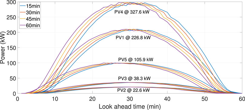
Figure 5. PV plants clustering in Summer.
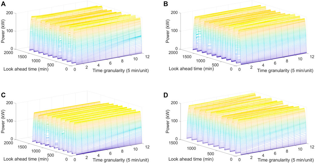
Figure 6. Multi-step power prediction evaluated with different optimization algorithm in four seasons: (A) spring, (B) summer, (C) autumn, and (D) winter.
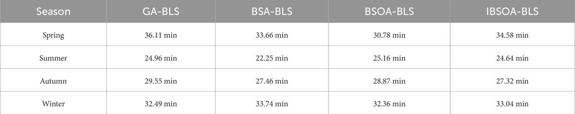
Table 5. Computation time of model training.
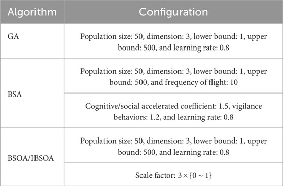
Table 6. Algorithm parameter settings.
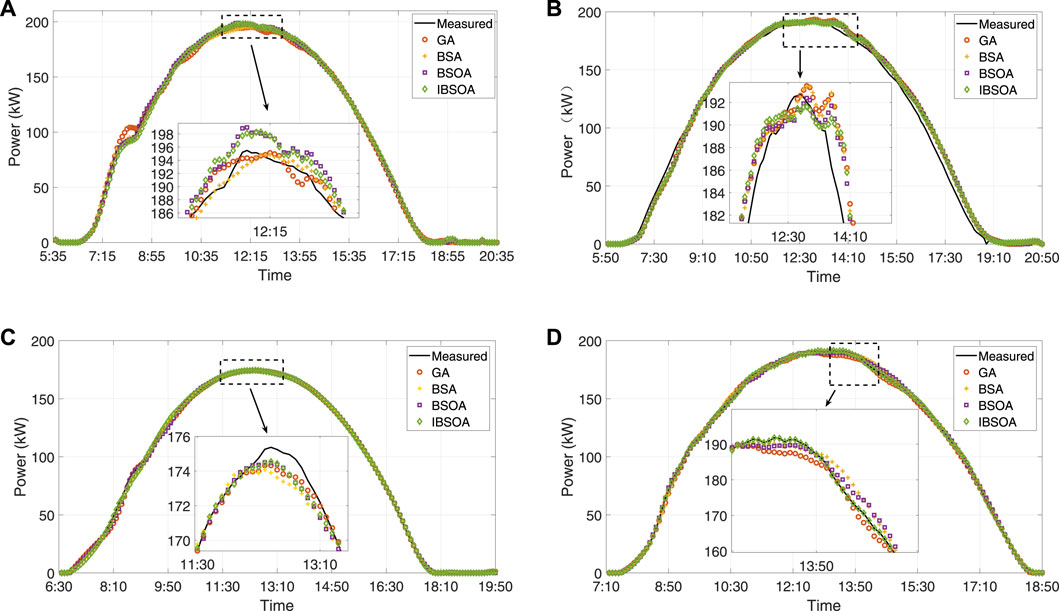
Figure 7. 1 h ahead power prediction evaluated with different optimization algorithm in four seasons: (A) Spring, (B) Summer, (C) Autumn, (D) Winter.
Table 7 indicates that the predictions made by these models exhibit slight deviations from the actual values. The RMSE indicators of the proposed prediction method are consistently lower than the worst-case scenario in each season, decreasing by 3.2283 kW in spring, 3.9159 kW in summer, 1.3425 kW in autumn, and 1.4058 kW in winter. Similarly, the MAPE exhibits a reduction compared to the worst case, with decreases of 0.882% in spring, 1.2399% in summer, 1.803% in autumn, and 1.087% in winter. The results demonstrate that, in general, the predictive performance of the proposed IBSOA-BLS model surpasses that of the other three models. The MAPE for the IBSOA-BLS model ranges from approximately 0.769%–1.639% across four seasons, which is lower than the results obtained by the other three models (GA-BLS, BSA-BLS, and BSOA-BLS). The MAPE in spring reaches 1.639% due to power fluctuation caused by cloud motion. Despite the differences arising from the regular and relatively low volatility in PV power generation on sunny days, compared to the other three models, IBSOA-BLS exhibits superior robustness, leading to prediction outcomes that closely align with the actual values. The quantified results of prediction errors are associated with four seasons. It reveals that on sunny days with stable power fluctuations, the IBSOA-BLS-based prediction method outperforms the other three models. All models exhibit small RMSE and MAPE values for prediction errors, indicating relatively accurate predictions. Among the four season simulations, the proposed IBSOA-BLS method exhibits lower error quantization values and superior predictive performance compared to the other three methods. It also demonstrates good adaptability to environmental conditions, especially on sunny days. Additionally, it is observed from the experimental error index values that once the input variables and structural parameters of the prediction model are determined, RMSE and MAPE values for GA-, BSA-, BSOA-, and IBSOA-based BLS methods remain consistent, indicating more accurate predictive performance for IBSOA-BLS. In contrast, when other methods are employed under the same conditions for multiple predictions, the results of each prediction exhibit varying amplitudes and lack stability. This is because the proposed method achieves an improved accuracy by considering both the mean and the best hyperparameters during the optimization process of IBSOA.
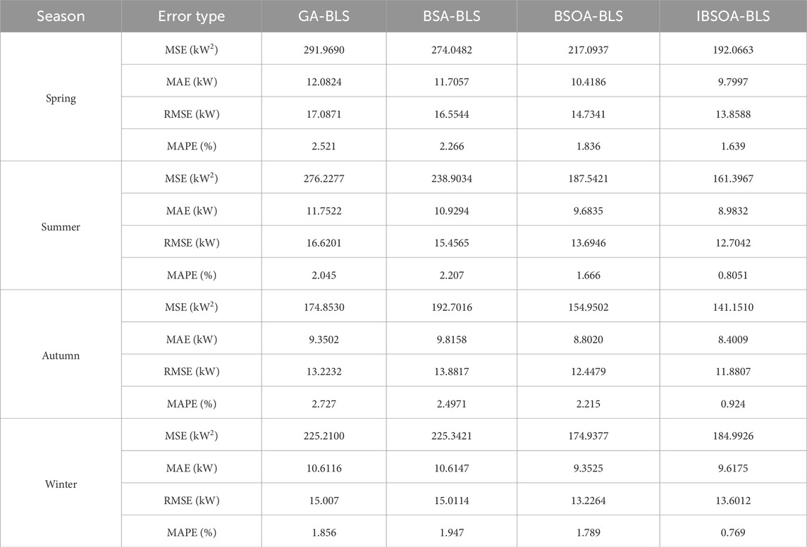
Table 7. Prediction performance under diverse algorithmic variants.
6 Conclusion
This paper proposes a PV power forecasting model based on BLS and IBSOA. Compared to the three other traditional algorithms (GA, BSA, and BSOA), which do not consider the historical experience and the representation of the characteristics of extensive data, IBSOA provides sufficient information during the evolution process to regulate the correct optimization search direction and maintain dynamic population diversity, thereby mitigating the risk of converging on the local optima. These improvements are achieved through enhancements to the selection and mutation processes of BSOA. BLS, which reduces extra network layers, effectively addresses the challenges posed by deep architecture in traditional neural networks when dealing with large-scale data forecasting. The SOM is utilized not only to cluster the five PV plants based on their respective external conditions but also to capture the spatio-temporal dependence of PV power generation under varying conditions. The effectiveness of the forecasting model is validated on the actual data on PV units from the DKA solar center in Australia. Based on well-tuned hyperparameters of BLS by IBSOA, the results indicate that the proposed PV power forecasting model yields more reliable and accurate predictions when compared to those produced by GA-BLS, BSA-BLS, and BSOA-BLS. The future work will concentrate on adding rainy days in each season for training and testing the model on more complex case studies.
Data availability statement
Publicly available datasets were analyzed in this study. These data can be found at: https://dkasolarcentre.com.au/locations/alice-springs.
Author contributions
WT: conceptualization, formal analysis, project administration, writing–original draft, and writing–review and editing. KH: data curation, investigation, methodology, software, supervision, validation, writing–original draft, and writing–review and editing. TQ: conceptualization, funding acquisition, methodology, resources, supervision, and writing–review and editing. WL: formal analysis, investigation, validation, visualization, and writing–review and editing. XX: investigation, resources, software, supervision, and writing–review and editing.
Funding
The author(s) declare that financial support was received for the research, authorship, and/or publication of this article. This work was supported in part by the National Natural Science Foundation of China (51977082), the Guangdong Basic and Applied Basic Research Foundation (2021A1515110675), the Guangzhou Science and Technology Plan Project (202201010577), and Fundamental Research Funds for the Central Universities (x2dl-D2221040).
Conflict of interest
The authors declare that the research was conducted in the absence of any commercial or financial relationships that could be construed as a potential conflict of interest.
Publisher’s note
All claims expressed in this article are solely those of the authors and do not necessarily represent those of their affiliated organizations, or those of the publisher, the editors, and the reviewers. Any product that may be evaluated in this article, or claim that may be made by its manufacturer, is not guaranteed or endorsed by the publisher.
Abbreviations
BLS, broad learning system; BSA, bird swarm algorithm; BSA-BLS, bird swarm algorithm-based broad learning system; BSOA, backtracking search optimization algorithm; BSOA-BLS, backtracking search optimization algorithm-based broad learning system; DM, Diebold–Mariano test; GA, genetic algorithm; GA-BLS, genetic algorithm-based broad learning system; IBSOA, improved backtracking search optimization algorithm; IBSOA-BLS, improved backtracking search optimization algorithm-based broad learning system; MAE, mean absolute error; MAPE, mean absolute percentage error; MSE, mean squared error; RMSE, root-mean-squared error; RVFLNN, random vector link neural network; SOM, self-organizing map; TOLO, topological opposition-based learning operator.
References
Ahmed, R., Sreeram, V., Mishra, Y., and Arif, M. (2020). A review and evaluation of the state-of-the-art in PV solar power forecasting: techniques and optimization. Renew. Sustain. Energy Rev. 124, 109792. doi:10.1016/j.rser.2020.109792
Aslam, M., Lee, S. J., Khang, S. H., and Hong, S. (2021). Two-stage attention over LSTM with bayesian optimization for day-ahead solar power forecasting. IEEE Access 9, 107387–107398. doi:10.1109/access.2021.3100105
Bamdad, K., Cholette, M. E., Guan, L., and Bell, J. (2017). Ant colony algorithm for building energy optimisation problems and comparison with benchmark algorithms. Energy Build. 154, 404–414. doi:10.1016/j.enbuild.2017.08.071
Barreto, G. A. (2007). “Time series prediction with the self-organizing map: a review,” in Perspectives of neural-symbolic integration (Singapore: Springer), 135–158.
Chen, C. P., and Liu, Z. (2017). Broad learning system: an effective and efficient incremental learning system without the need for deep architecture. IEEE Trans. neural Netw. Learn. Syst. 29, 10–24. doi:10.1109/tnnls.2017.2716952
Cheng, Y., Le, H., Li, C., Huang, J., and Liu, P. X. (2022). A decomposition-based improved broad learning system model for short-term load forecasting. J. Electr. Eng. Technol. 17, 2703–2716. doi:10.1007/s42835-022-01127-x
Choi, J., Lee, J. I., Lee, I. W., and Cha, S. W. (2021). Robust PV-BESS scheduling for a grid with incentive for forecast accuracy. IEEE Trans. Sustain. Energy 13, 567–578. doi:10.1109/tste.2021.3120451
Civicioglu, P. (2013). Backtracking search optimization algorithm for numerical optimization problems. Appl. Math. Comput. 219, 8121–8144. doi:10.1016/j.amc.2013.02.017
Deniz, E., Aydogmus, O., and Aydogmus, Z. (2016). Implementation of ANN-based selective harmonic elimination PWM using hybrid genetic algorithm-based optimization. Measurement 85, 32–42. doi:10.1016/j.measurement.2016.02.012
Diebold, F. X. (2015). Comparing predictive accuracy, twenty years later: a personal perspective on the use and abuse of Diebold–Mariano tests. J. Bus. Econ. Statistics 33, 1. doi:10.1080/07350015.2014.983236
Ding, S., Xu, X., Zhu, H., Wang, J., and Jin, F. (2011). Studies on optimization algorithms for some artificial neural networks based on genetic algorithm (GA). J. Comput. 6, 939–946. doi:10.4304/jcp.6.5.939-946
Fekri, M. N., Patel, H., Grolinger, K., and Sharma, V. (2021). Deep learning for load forecasting with smart meter data: online adaptive recurrent neural network. Appl. Energy 282, 116177. doi:10.1016/j.apenergy.2020.116177
Feng, Q., Liu, Z., and Chen, C. P. (2022). Broad and deep neural network for high-dimensional data representation learning. Inf. Sci. 599, 127–146. doi:10.1016/j.ins.2022.03.058
Ghofrani, M., Ghayekhloo, M., Arabali, A., and Ghayekhloo, A. (2015). A hybrid short-term load forecasting with a new input selection framework. Energy 81, 777–786. doi:10.1016/j.energy.2015.01.028
Gong, X., Zhang, T., Chen, C. L. P., and Liu, Z. (2022). Research review for broad learning system: algorithms, theory, and applications. IEEE Trans. Cybern. 52, 8922–8950. doi:10.1109/tcyb.2021.3061094
Hafeez, G., Alimgeer, K. S., and Khan, I. (2020b). Electric load forecasting based on deep learning and optimized by heuristic algorithm in smart grid. Appl. Energy 269, 114915. doi:10.1016/j.apenergy.2020.114915
Hafeez, G., Khan, I., Jan, S., Shah, I. A., Khan, F. A., and Derhab, A. (2021). A novel hybrid load forecasting framework with intelligent feature engineering and optimization algorithm in smart grid. Appl. Energy 299, 117178. doi:10.1016/j.apenergy.2021.117178
Hafeez, G., Khan, I., Usman, M., Aurangzeb, K., and Ullah, A. (2020a). “Fast and accurate hybrid electric load forecasting with novel feature engineering and optimization framework in smart grid,” in 2020 6th Conference on Data Science and Machine Learning Applications (CDMA), Riyadh, Saudi Arabia, 4th to 5th March 2020, 31–36.
Hassan, B. A., and Rashid, T. A. (2020). Operational framework for recent advances in backtracking search optimisation algorithm: a systematic review and performance evaluation. Appl. Math. Comput. 370, 124919. doi:10.1016/j.amc.2019.124919
Hossain, M. S., and Mahmood, H. (2020). Short-term photovoltaic power forecasting using an LSTM neural network and synthetic weather forecast. IEEE Access 8, 172524–172533. doi:10.1109/access.2020.3024901
Hu, R., Hu, W., Gökmen, N., Li, P., Huang, Q., and Chen, Z. (2019). High resolution wind speed forecasting based on wavelet decomposed phase space reconstruction and self-organizing map. Renew. Energy 140, 17–31. doi:10.1016/j.renene.2019.03.041
Hu, W., Zhang, X., Zhu, L., and Li, Z. (2020). Short-term photovoltaic power prediction based on similar days and improved SOA-DBN model. IEEE Access 9, 1958–1971. doi:10.1109/access.2020.3046754
Khuntia, S. R., Rueda, J. L., and van Der Meijden, M. A. (2016). Forecasting the load of electrical power systems in mid-and long-term horizons: a review. IET Generation, Transm. Distribution 10, 3971–3977. doi:10.1049/iet-gtd.2016.0340
Kleissl, J. (2013). Solar energy forecasting and resource assessment. San Diego, USA: University of California. Press, 178–182.
Kohonen, T. (2013). Essentials of the self-organizing map. Neural Netw. official J. Int. Neural Netw. Soc. 37, 52–65. doi:10.1016/j.neunet.2012.09.018
Konjić, T., Jahić, A., and Pihler, J. (2015). “Artificial neural network approach to photovoltaic system power output forecasting,” in 2015 18th Intelligence Systems Applications to Power Systems (ISAP), Porto, Portugal, 11-16 September 2015 (Porto, Portugal: IEEE).
Li, G., Liu, C. X., Liao, S. L., and Cheng, C. T. (2015). Applying a correlation analysis method to long-term forecasting of power production at small hydropower plants. Water 7, 4806–4820. doi:10.3390/w7094806
Li, W., Qian, T., Zhang, Y., Shen, Y., Wu, C., and Tang, W. (2023a). Distributionally robust chance-constrained planning for regional integrated electricity–heat systems with data centers considering wind power uncertainty. Appl. Energy 336, 120787. doi:10.1016/j.apenergy.2023.120787
Li, W., Qian, T., Zhao, W., Huang, W., Zhang, Y., Xie, X., et al. (2023b). Decentralized optimization for integrated electricity–heat systems with data center based energy hub considering communication packet loss. Appl. Energy 350, 121586. doi:10.1016/j.apenergy.2023.121586
Lin, G. Q., Li, L. L., Tseng, M. L., Liu, H. M., Yuan, D. D., and Tan, R. R. (2020). An improved moth-flame optimization algorithm for support vector machine prediction of photovoltaic power generation. J. Clean. Prod. 253, 119966. doi:10.1016/j.jclepro.2020.119966
McAleer, M., and Medeiros, M. C. (2011). Forecasting realized volatility with linear and nonlinear univariate models. J. Econ. Surv. 25, 6–18. doi:10.1111/j.1467-6419.2010.00640.x
Montgomery, D. C., and Runger, G. C. (2017). Applied statistics and probability for engineers. New Jersey, United States: John Wiley & Sons.
Oudjana, S., Hellal, A., and Mahammed, I. H. (2013). Power forecasting of photovoltaic generation. Int. J. Electr. Comput. Eng. 7, 627–631. doi:10.5281/zenodo.1333286
Pedro, H. T., and Coimbra, C. F. (2012). Assessment of forecasting techniques for solar power production with no exogenous inputs. Sol. Energy 86, 2017–2028. doi:10.1016/j.solener.2012.04.004
Qian, T., Liu, Y., Zhang, W., Tang, W., and Shahidehpour, M. (2020). Event-triggered updating method in centralized and distributed secondary controls for islanded microgrid restoration. IEEE Trans. Smart Grid 11, 1387–1395. doi:10.1109/tsg.2019.2937366
Rahman, M. M., Shakeri, M., Khatun, F., Tiong, S. K., Alkahtani, A. A., Samsudin, N. A., et al. (2023). A comprehensive study and performance analysis of deep neural network-based approaches in wind time-series forecasting. J. Reliab. Intelligent Environ. 9, 183–200. doi:10.1007/s40860-021-00166-x
Shaqour, A., Ono, T., Hagishima, A., and Farzaneh, H. (2022). Electrical demand aggregation effects on the performance of deep learning-based short-term load forecasting of a residential building. Energy AI 8, 100141. doi:10.1016/j.egyai.2022.100141
Viet, D. T., Phuong, V. V., Duong, M. Q., and Tran, Q. T. (2020). Models for short-term wind power forecasting based on improved artificial neural network using particle swarm optimization and genetic algorithms. Energies 13, 2873. doi:10.3390/en13112873
Wang, H., Zeng, K., Liu, J., Lin, B., Du, B., and Tang, S. (2020). Broad learning for short-term low-voltage load forecasting. 2020 International Conference on Smart Grids and Energy Systems (SGES), Perth, Australia, 23-26 November 2020 (Perth, Australia: IEEE).
Yang, K., Liu, Y., Yu, Z., and Chen, C. P. (2021). Extracting and composing robust features with broad learning system. IEEE Trans. Knowl. Data Eng. 35, 3885–3896. doi:10.1109/tkde.2021.3137792
Yildiz, C., Acikgoz, H., Korkmaz, D., and Budak, U. (2021). An improved residual-based convolutional neural network for very short-term wind power forecasting. Energy Convers. Manag. 228, 113731. doi:10.1016/j.enconman.2020.113731
Zhou, N., Xu, X., Yan, Z., and Shahidehpour, M. (2022). Spatio-temporal probabilistic forecasting of photovoltaic power based on monotone broad learning system and copula theory. IEEE Trans. Sustain. Energy 13, 1874–1885. doi:10.1109/tste.2022.3174012
Zhou, X., Chen, L., Yan, J., and Chen, R. (2020). Accurate DOA estimation with adjacent angle power difference for indoor localization. IEEE Access 8, 44702–44713. doi:10.1109/access.2020.2977371
Zhu, Y., Xu, X., Yan, Z., and Lu, J. (2022). Data acquisition, power forecasting and coordinated dispatch of power systems with distributed pv power generation. Electr. J. 35, 107133. doi:10.1016/j.tej.2022.107133
Appendix A: Optimization testbench.
f1: Branin function: http://www.sfu.ca/ssurjano/branin.html.
f2: Gramacy and lee function: http://www.sfu.ca/ssurjano/grlee08.html.
f3: Currin et al. exponential function: http://www.sfu.ca/ssurjano/curretal88exp.html.
f4: Lim et al. polynomial function: http://www.sfu.ca/ssurjano/limetal02non.html.
f5: Dette and Pepelyshev exponential function: http://www.sfu.ca/ssurjano/detpep10exp.html.
f6: Friedman function: http://www.sfu.ca/ssurjano/fried.html.
f7: Dette and Pepelyshev eight-dimensional function: http://www.sfu.ca/ssurjano/detpep108d.html.
f8: Welch et al. function: http://www.sfu.ca/ssurjano/emulat.html.
Appendix B: Diebold–Mariano test
The Diebold–Mariano (DM) test serves as a statistical tool for comparing the predictive accuracy of two models in time series analysis. Focused on mean squared forecast errors, the test evaluates whether one model outperforms the other. By calculating the DM test statistic, which considers the variance of the difference in mean squared errors, it determines the superiority of one model over the other (Diebold, 2015). A positive DM test statistic signifies that the first input model exhibits lower mean squared forecast errors, indicating better predictive performance. Conversely, a negative value suggests superior performance for the second input model. Furthermore, in conjunction with the DM test, a p-value is frequently evaluated, which reflects the extent of extremeness in the probability of observing a test statistic compared to the one calculated from the sample, assuming the null hypothesis (Montgomery and Runger, 2017) is true. The p-value is computed by comparing the DM test value to the standard normal distribution. The significance level, denoted by αs normally set at 0.01, 0.05, or 0.1 (McAleer and Medeiros, 2011), is a critical component in hypothesis testing that influences the decision-making process, regarding the null hypothesis. Before using the DM test, it is essential to check if the prediction errors are serially uncorrelated and of constant variance. In this study, the DM test is performed for the prediction accuracy by the following steps:
1. Generate predicted power errors: obtain the prediction errors from two different models by subtracting the measured values from the predicted outcomes.
2. Calculate squared predicted power errors: square each prediction error to eliminate the effects of positive and negative errors.
3. Calculate mean squared predicted power errors: find the average of the squared predicted power errors for each model.
4. Calculate the test statistic: the Diebold–Mariano test statistic is calculated as the difference between the mean squared predicted power errors of the two models, divided by a measure of the variance of this difference. The formula is expressed as follows:
where D represents the DM test statistic,
5. Calculate the p-value: standardize the DM value by dividing it by its standard error υ and then compare it to the standard normal as follows:
where p represents the probability of a null hypothesis based on measured data,
It should be noted that the desired level of confidence (αs) is set to 0.1 in this study, indicating 10% margin of error, and it is distributed equally in the sampling distribution. If the p-value falls below the specified significance level, it supports the rejection of the null hypothesis, indicating a significant difference in forecast accuracies for the compared models. On the contrary, a higher p-value suggests that the observed differences in prediction accuracy might be due to random variation, which implies the need for potential adjustments or exploration to the model DM test evaluation and interpretation for (Table 8–Table 10).
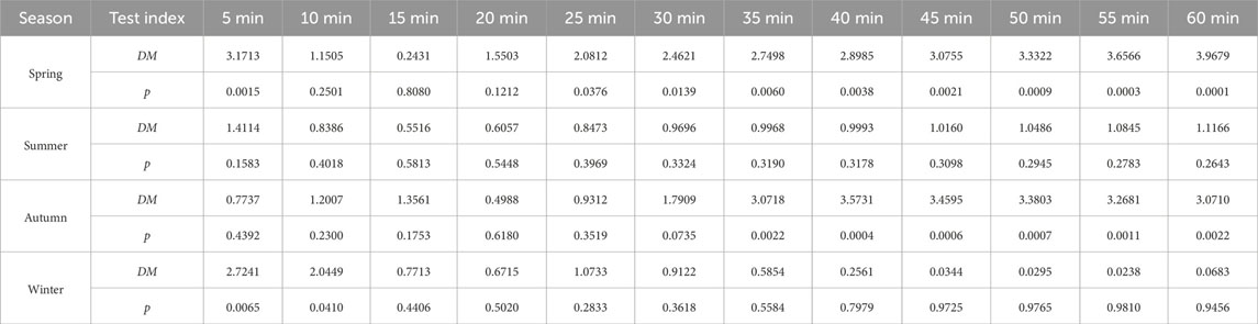
TABLE 8. Prediction evaluation of IBSOA-BLS and GA-BLS assessed by the Diebold–Mariano test.
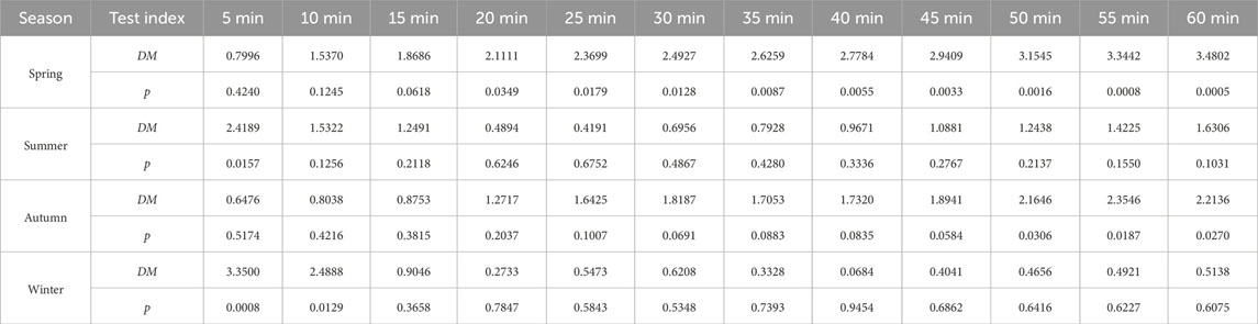
TABLE 9. Prediction evaluation of IBSOA-BLS and BSA-BLS assessed by the Diebold–Mariano test.
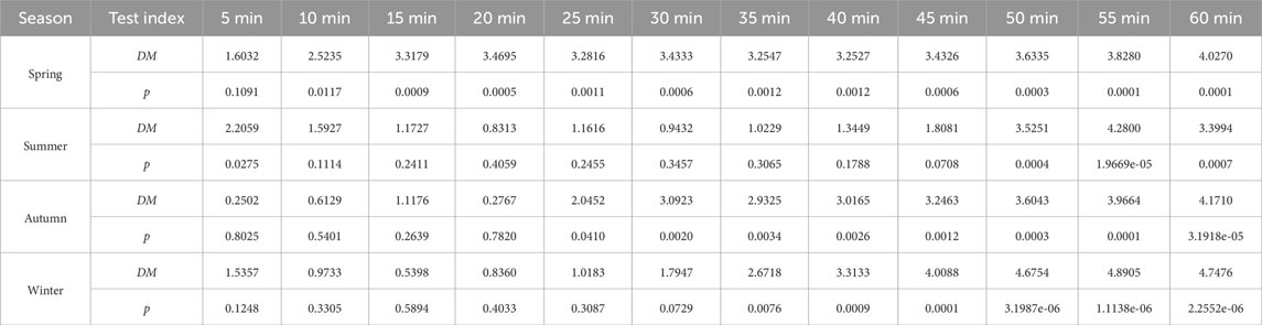
TABLE 10. Prediction evaluation of IBSOA-BLS and BSOA-BLS assessed by the Diebold–Mariano test.
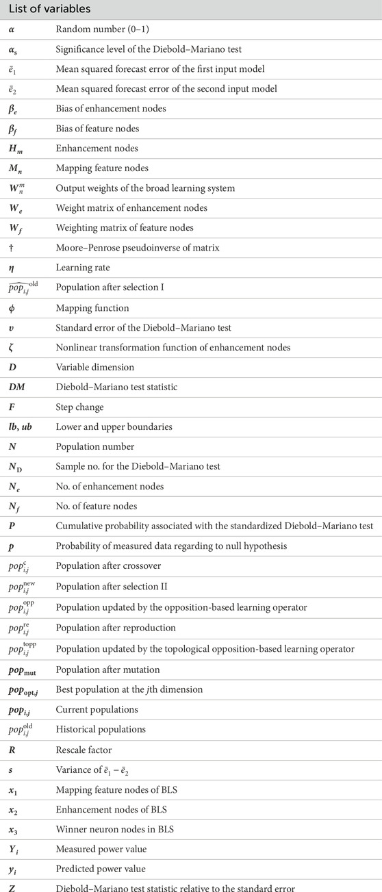
Nomenclature
Keywords: photovoltaic power forecasting, improved backtracking search optimization algorithm, broad learning system, deep neural network, hyperparameter optimization
Citation: Tang W, Huang K, Qian T, Li W and Xie X (2024) Spatio-temporal prediction of photovoltaic power based on a broad learning system and an improved backtracking search optimization algorithm. Front. Energy Res. 12:1343220. doi: 10.3389/fenrg.2024.1343220
Received: 28 November 2023; Accepted: 19 February 2024;
Published: 20 March 2024.
Edited by:
Ali Bassam, Universidad Autónoma de Yucatán, MexicoReviewed by:
Linfei Yin, Guangxi University, ChinaMansoor Khan, Qilu Institute of Technology (QIT), China
Copyright © 2024 Tang, Huang, Qian, Li and Xie. This is an open-access article distributed under the terms of the Creative Commons Attribution License (CC BY). The use, distribution or reproduction in other forums is permitted, provided the original author(s) and the copyright owner(s) are credited and that the original publication in this journal is cited, in accordance with accepted academic practice. No use, distribution or reproduction is permitted which does not comply with these terms.
*Correspondence: Tong Qian, cWlhbnRvbmdAc2N1dC5lZHUuY24=