Why germanys energiewende may fail to meet its goals: insights from power system simulation with natural generation

In order to achieve the Paris climate targets, the German government has developed phased plans and anchored these in an amendment to the Renewable Energy Sources Act (EEG). This not only defines expansion targets for renewable energy producers, but also the additional amounts of energy that must be available in the electricity grid in future if it is to supply the mobility and building heating sectors, which are currently still powered by fossil fuels. While the lack of grid transport capacities is recognized and discussed in the public debate, another known and critical hurdle is rarely presented here. This is the temporal distribution of power from renewable energies and its effects on the processes involved in controlling the grid balance. By analyzing a target scenario specified in the EEG for 2030 and another for 2040+, which a German economic research institute recommends to policymakers, the aim is to investigate whether their targets can be achieved under the conditions of the natural fluctuations occurring in Germany and the quantities of renewable energy that can be harvested with a reasonable use of resources. The focus is on simulating future generation curves using historical data in such a way that they show the typical weather-driven behaviour to be expected in Germany. Unavoidable Surplus generation is used as efficiently as possible with electricity and hydrogen storage systems. Both scenarios fall considerably short of their targets. CO2-free coverage of the demand specified for the long-term future is only possible with a quantity of generators that is at the limit of what is feasible. The reason for this is that the current plans are obviously based on an unrealistic picture of the temporal distribution of renewable energy output. Achieving the transformation goals in Germany could be much more complex than politicians currently believe and may require a change in strategy sooner or later.

1 Introduction, aim of the work

In order to achieve the goals to which the German government has committed itself as part of the Paris Climate Agreement, it has defined expansion stages of the German energy transition and published them as part of the latest amendment to the Renewable Energy Sources Act (EEG). These define, in almost annual increments, which energy segments that are currently still powered by fossil fuels, such as building heating and electromobility, are to be supplied via the electricity grid in the future through sector coupling, how electricity demand is to develop as a result, and what generation capacity is to be installed for this purpose.

The aim of the study presented here is to analyse the consistency of these requirements. In other words: Can the required supply be achieved with the specified generators? This is not a matter of course, as the characteristics of wind and solar power differ significantly from those of fossil and nuclear power plants in two respects.

Firstly, their power flow is subject to temporal fluctuations, the distribution of which follows different typical patterns for sun and wind. Unlike conventional turbogenerators, their output cannot be controlled, except to limit or shut down. As the consumption and production capacities in an electricity network must always be exactly balanced, their energy cannot be used alone without further measures; there is always either a surplus or a shortfall.

Second, while conventional power plants were built close to their customers, renewable energy producers are widely dispersed and much smaller in terms of individual output than conventional power plants. The largest amounts of wind power come from the coastal regions of northern Germany, while solar energy is more productive in the sunnier south and south-west.

The resulting high demand for additional transport network capacity has long been part of the public debate in Germany. In contrast, less is heard about the fluctuations of renewable energy producers and their integration into the electricity grid, even though they could pose a greater risk to the success of the energy transition than the transport problem. This paper therefore focuses on the consequences of the physical minimum condition of grid equilibrium. It should always be noted that this is a necessary but not a sufficient condition for the success of the energy system transformation, as transport constraints, which are deliberately not considered in depth, are by no means negligible. Transport bottlenecks will always exacerbate the results of the analyses presented here.

Generation fluctuations have the same effect on the grid balance as consumption fluctuations, except for the sign. With increasing size, they do not require a different type of control system, but increasingly more control power. Before the introduction of renewable generators, disturbances in the balance between generation and consumption were mainly caused by daily fluctuations in consumer output. These occurred predictably on a daily and weekly basis, so the grid balance was constantly adjusted by matching generator output to the target output set by the consumers. Even then, the grid control systems used before the era of renewable energy generation were not trivial, as they always had to be able to cope with the failure of large resources, such as power plants or transmission lines, without jeopardising the stability of the grid. Today, the impact of fluctuations in renewable generation on the grid balance is much greater than that of consumers. Since renewable generators cannot be controlled, they can only be operated in combination with conventional turbines whose output can be quickly adjusted.

Today, deviations are actively compensated by a system of power plants that intervene with balancing power in different time cascades and priorities ranging from seconds to minutes to hours. A large increase in the share of renewable energy producers will require the provision of much more balancing power, but this is not the subject of this paper. The simple assumption here is that these issues can be resolved and that stable grid control procedures and resources will be available for a future grid.

However, even a perfectly functioning grid control system does not change the consequences of using fluctuating power to supply a defined load curve. Moreover, it can only work with the resources available to it. We must therefore include flexible consumers such as electrical storage, hydrogen storage, etc. in the analysis. As it is ultimately important to produce electricity at an attractive and affordable cost, the focus here will be on the resulting annual energy balances and thus the economic viability of such a system in different configurations. These energy balances are the necessary basis for subsequent cost estimates. In the course of this work it will be shown that the temporal power distribution of the fluctuating generators has a significant influence on the costs incurred for covering the consumer power curve. A key indicator of this is the residual power that still needs to be supplied by turbines. A realistic simulation depends heavily on a realistic and true-to-nature representation of the fluctuations.

The distribution functions of energy from wind and sun have been known for a long time. Having realistic model parameters that apply to a defined geographical area with a specific expansion status is another matter.

For this reason, offline full-year simulations are used here, based on historical generation patterns from real weather years, whose raw data are transformed to the installed capacity of the respective future year. The simulation is limited to determining the partial components of power that are inevitably generated as a result of functioning grid control. These are then used differently and subjected to an annual balance.

We will see that the key to achieving the targets is to minimise the annual so-called “residual work,” as this must be generated either from hydrogen, which is preferably generated from surplus production and does not need to be purchased, or from fossil fuels, which makes it more difficult to achieve the CO2 emission targets.

The study focuses on two scenarios. One for the 2030 milestone of the energy system transformation, as defined by the Renewable Energy Act (BMJ, 2023), in which the expanded electricity grid is to supply 80% RE. The other is a 100% RE scenario, as proposed to the German government in 2021 for the period after 2040 in Policy Recommendation 167 (Kendziorski et al., 2021) by the German Institute for Economic Research Berlin (DIW) and published separately in its weekly reports (Göke et al., 2021).

2 Materials and methods

2.1 State of the art

Since the late 1970 s, there has been a great deal of work on the variability of wind power in particular. The Weibull distribution has become established for modelling these fluctuations, e.g., Bowden et al. (1983) and Stevens and Smulders (1979). Ahlborn (2015) investigated whether a large number of generators with a Weibull distribution can smooth the energy flow generated by wind turbines. Using appropriate mathematical theory and real data, he shows that the total output of a large number of wind turbines does not have a lower variance compared to a small number, even if they are all statistically independent from each other, there is no real smoothing of the power curve. In the case of critical weather phenomena, such as large, stable high-pressure systems, it becomes even more difficult because wind turbines are correlated even on a European scale. Ahlborn (2023) shows the critical conditions for using excess generation for Power-t-X conversion, as a large part of its energy is contained in short but very high power peaks.

The so-called “Acatech study” (Ausfelder, 2017) on sector coupling was presented as a joint project of three renowned technical academies, a comprehensive study on the challenges of the German energy transition, which looked quite deep at many aspects, including the main challenges of dealing with fluctuating generators. Among other things, it has already been stated here that even with the highest level of RE expansion, there will still be too many supply gaps to be able to allocate secure power to solar and wind, and that there will still be a need to provide standby power from conventional turbines at full consumer peak power (Ausfelder, 2017, p. 36).

Existing storage facilities in Germany currently only have a limited capacity of 40 GWh as pumped storage with no significant growth potential. Battery storage systems exist worldwide as pilot plants, e.g., the Moss Landing Energy Storage Facility in Monterey with a capacity of 1.6 GWh and an output of 400 MW. As electrical storage systems are still far from acceptable costs, an important aspect is how much excess energy can be economically shifted to times of residual demand with how little storage.

Werner Sinn (2017) has pointed out the limits of the use of volatile energy, based on annual observations with real generation in the German grid. Using concrete examples of demand management (shifting consumption), he shows that only a very limited part of consumer demand can be shifted to times of surplus. His conclusion: A future German electricity system with a high share of renewables will not be able to use large amounts of volatile energy unless it has storage capacity in the order of terawatt hours (TWh).

A team of authors from the German Institute for Economic Research (DIW Berlin) disagrees (Schill et al., 2018) and accuses Sinn of having methodological weaknesses, describing unrealistic borderline cases and emphasising that the required storage capacities could be one to two orders of magnitude smaller if “moderate curtailment of RE peaks is permitted,” but does not show a 100% scenario for this. However, another paper by the same authors (Zerrahn et al., 2018; Figure 6) clearly shows that the statement about one to two orders of magnitude lower storage requirements only applies to electricity systems with low RE shares. The 80% scenario presented there alone requires a capacity requirement of 1.7 TWh despite a more than moderate curtailment of 30% of the total annual generation and thus actually confirms that Sinn’s analysis is not too wrong.

The DIW study cited above (Kendziorski et al., 2021) describes and recommends to German policymakers a simulation system that exploits the potential for RE expansion in Germany to a greater extent than specified in the EEG for 2040. According to the authors, it is based on the AnyMod model framework of the TU Berlin (Göke, 2021), within which Germany is modelled as part of the European interconnected grid. Electricity is balanced in 1-h cycles, heat in 4-h cycles and hydrogen in 1-day cycles; imports and exports are used to enable balancing with neighbouring countries. Hydrogen imports/exports are allowed in any quantity. The assumed energy demand for Germany is taken from the openENTRANCE project and consists of 1,070 TWh of electricity and 139 TWh of hydrogen for processes that are difficult to electrify. The study compares sub-scenarios, considering a more centralised and a more decentralised model, and evaluates their consequences in terms of different resource requirements, such as grid transport. In particular, the DIW study emphasises that its system approach for Germany also works in times of lowest generation and supports this with a time-power diagram of a winter week, which is shown here with permission (Figure 1).

FIGURE 1

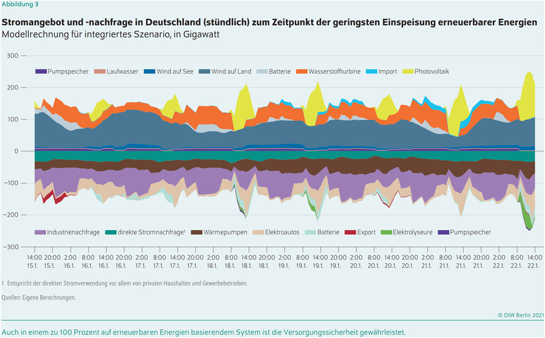
FIGURE 1. Electricity supply and demand in Germany at the time of lowest generation according to the DIW Study (Göke et al., 2021) “100% Erneuerbare Energien für Deutschland“ Source Deutsches Institut für Wirtschaftsforschung Berlin.

Prior to the DIW study, the Fraunhofer Institute for Solar Energy Systems (ISE) in Freiburg had already published a similar study (Philip, 2020) with a slightly different focus on the future development of the German energy system. Depending on how much wind and solar energy is acceptable to society, it describes various scenarios and their possible consequences on the way to a 100% renewable energy supply.

This study also looks at operation with fluctuating generators and describes different situations as power curves for critical weeks of the year (e.g., pp. 31, 32).

2.2 Approach to testing the physical feasability of the scenarios

2.2.1 General needs and premises

The purpose of sector coupling is to use directly generated electrical energy from the sun and wind to bypass the conversion processes of conventional thermal power plants, where 50%–70% of the primary energy is lost as waste heat. This study will focus on those conversion processes that are necessary to provide the electrical energy quantities required by the scenario being analyzed. The supply is to come from fluctuating generation, whose installed capacities correspond to the scenario specifications and whose fluctuations are to follow the temporal course of real weather years in Germany. The representation of a realistic and statistically correct time course of the total RE output is therefore an essential pillar of this work.

The behavior of electricity consumers is also linked to the balance of the grid. The reference value for the control of the grid balance is currently dictated by the consumers by switching on and off electrical loads, and it is the responsibility of the grid operator to match this exactly with the required generation. With fluctuating generation, at any given time there is either a power deficit that needs to be filled with traditional turbo generators, or there is excess generation that either needs to be quickly found a consumer for, or needs to be curtailed.

One way to avoid curtailment of available power is to shift consumption to times of surplus through demand management. So-called flexible consumers do not decide when to use electricity, but are allocated it while they are in a waiting position. As we will see later, overgeneration is often characterized by high, short power peaks whose energy content is by no means negligible, but whose maximum values lead to poor utilization rates that hardly amortize high investments such as batteries or electrolyzers. The storage of process heat on time scales of days may offer some potential here. In order to avoid huge transport network demands at these peaks, this will often mean that sources and consumers need to be close to each other. However, where and how such industrial relocation and restructuring will pay off and take place in the near future must be decided by the companies concerned; it is neither foreseeable nor calculable today. To avoid having to make speculative assumptions about demand management, the following assumptions are used here.

- Whatever new work and production structures emerge in the future, the demand for competitiveness will lead to some form of good and even utilization of human and machine resources, and thus the need for regular and reliable supply will continue to exist. This means that the majority of electricity demand will continue to be requested at traditional times, resulting in an electricity load curve that includes today’s daily, weekly, and other seasonal periods. Therefore, we take the basic shape of the load curve of the reference year and adapt it to the annual amount of energy to be supplied in the scenario to be analyzed.

- Furthermore, it is assumed so far that flexible consumers will be primarily battery storage systems and hydrogen electrolysers.

- We are aware that there is further potential here that we cannot quantify today. Perhaps it will be possible to use the simulation results to identify desirable flexibilisation of customers at a later stage.

When it comes to real investments to implement the energy transition, absolute cost estimates will be necessary and important. However, we will not discuss absolute costs here, as these are still speculative. Instead, we will look at performance indicators from the annual balance sheet, the utilisation of key resources such as turbines, batteries or electrolysers. In particular, we will look at how much surplus energy from fluctuations can cover the required residual energy and whether the annual run of a scenario ends with a profit or a loss. These figures will tell us a lot and form the basis for future more precise cost derivation.

Before we describe the procedure for simulating a scenario in more detail, let’s take a closer look at where weather years are similar and different.

2.2.2 Description of static parameters and the fluctuations of RE generators

Most descriptions of RE generators refer to their installed capacity and annual energy output. In electrical engineering, the term utilization rate is used for variable output over a billing period. It is a dimensionless number that describes the ratio of the highest peak power to the average power during that time. Electricity customers who, like others, use a small amount of electricity each year, but demand ten times the average instantaneous power for short periods, require ten times the infrastructure of wires and transformers for almost the same amount of energy paid for. That’s why they get a surcharge on the tariff, which takes into account the resulting higher infrastructure requirements and their poor utilization. Fluctuating generators pose the same challenges for grid operators. For annual balances, the term annual full load hours is commonly used, which is calculated by multiplying the load factor by the number of hours in a year, as seen in Eqs 1, 2.

$AnnualEnergy=InstalledCapacity*UtilisationRate*24*365(1)$

$AnnualEnergy=InstalledCapacity*AnnualFullLoadHours(2)$

The term “annual full-load-hours” expresses in other words, how many hours the plant would be utilised if its annual yield were to occur continuously at nominal output.

In the case of resources whose utilization can be influenced, such as turbo generators, the aim is to use them as much as possible in order to minimize capital and fixed costs.

In contrast to that, the utilisation rates of RE generators are determined by nature and their installation location. Once they have been installed, the degree of utilisation can no longer be influenced except by curtailing or switching them off. Typical rough averages across Germany are 0.1 for solar, 0.2 for onshore wind, 0.45 for offshore wind. These figures give rise to a further challenge for the energy transition, which will not be pursued here, but which is also worth mentioning because it is rarely discussed. In a region where mainly solar energy is generated, the distribution and medium-voltage lines must therefore be designed for ten times the average annual power generated there; for wind it is around a factor of five.

Together with the installed capacity, the utilisation resp. annual-full-load-hours of RE Generators provide information about the amount of energy to be expected annually, however it says nothing about how this energy is distributed over the year.

In order to create realistic conditions, the idea here is to approximate “real weather” using historical data sequences from a reference year, which is extrapolated to the installed capacities of the target scenario.

An interesting question in this context is to what extent a selected weather year can be representative and how it can be categorised in comparison to other years. Another aspect is, will the yields of future generators improve vs. the historic ones in a way that it should be considered here.

A study by the IAEW at RWTH Aachen University (Schwaeppe et al., 2022) has analysed the first question for a German grid operator, forecasting the yields of wind and solar power plants for the period up to 2027. The study estimates which plants with which characteristics are likely to be retired and which new plants will be added. It is also based on weather observations in Germany since 1958, while trend scenarios and upper/lower corridors are derived from generation in the period 2011–2021. With the permission of the IAEW, two tables from this study are shown as graphs in Figure 2.

FIGURE 2

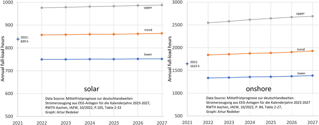
FIGURE 2. Development of full load hours for Onshore wind and solar generation in Germany according to IAEW-Study [13].

What they tell us:

- In General, the expected increases in full load hours are marginal in relation to the usual weather variations within a decade.

- With respect to the trend scenario, the upper/lower solar corridors are about +/− 14%, while there is no significant improvement in utilization or annual full load hours. The authors expect slightly higher values from ground-mounted solar parks due to better orientation compared to rooftop panels

- The wind situation is different, with +40%–30%, the expected variation corridors against the trend scenario are significantly higher, probably due to the v³ dependency between wind speed and electrical power. There is also some improvement in utilization, not due to technological improvements, but to the replacement of older wind turbines with higher ones that benefit from higher wind speeds. However, the shown improvement is marginal so far with less than 20 full load hours per year. For the 2030 scenario, this results in a small improvement from 1839 to 1992 h onshore. In contrast to the large weather variations that can be expected, we are on the verge of fictitious accuracy here.

The question is, if such development will accelerate or decelerate beyond 2030.

A study conducted by Deutsche Windguard on behalf of two industry associations in the wind power sector examines the complex influences on the long-term development of expected full load hours (Borrmann et al., 2020). They consider higher full load hours up to 3,000 as possible, but only in certain regions. For a high installed capacity in Germany in the range of 200 GW, where also many sites with moderate yields have to be occupied, the study sees a potential with 40,000 turbines and an annual yield of 500 TWh, which corresponds to 2,500 full load hours.

2.2.3 Timely power distribution of RE Generation in Germany

A widespread idea of future RE generation, both in politics and apparently also in parts of science, seems to be to set up such a large number of RE generators that their total output power hardly falls below the consumer need, even in times of low generation. Grid control will thus become a simple matter of curtailing RE generation or diverting it to local electrolysers to produce hydrogen from the abundant surpluses so that turbines only need to intervene in extreme situations.

A closer look at the nature of the fluctuations will show that this idea is far from reality. Instead of working with the commonly used load duration curves, we will use the histogram tool, which shows the same relationship more clearly. The statements we make here are not generally valid, but show the behavior of systems as they have been installed in Germany in recent years.

The power sum of the RE output is a superposition of the Weibull distributed wind power and solar power modulated by cloud cover and the day/night rhythm of our rotating planet. The histograms in Figure 3 show the time distribution of total instantaneous power for the years 2019–2022 in Germany. The data source for this analysis is the SMARD, 2023 portal of the Federal Network Agency. Since the installed capacity of each energy type is different in each of the last years due to the continuous expansion of renewable energy generation, the raw data has to be transformed to identical capacities for comparability. All annual curves in Figure 3 correspond to the installed capacities of the second scenario considered here.

FIGURE 3

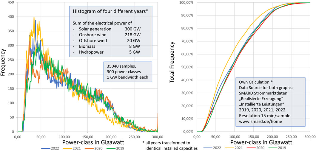
FIGURE 3. Comparison of 4 years’s annual power distribution, all transformed to the same installed Power of RE Generators.

With a sampling interval of 15 min, the year is represented by 35,040 or 35,136 data points with a power range of 0–300 GW. According to its instantaneous power each data point is assigned to one of 300 power classes with a bandwidth of 1 GW.

The histogram on the left shows the frequency per class plotted against power class. It shows how many of the annual data samples spend their time in a given power interval. On the right is the total frequency. Here we can see on the ordinate how much of the year the power curve is below the power threshold on the abscissa. For 50 GW, this varies from a total of 21% (77 days) to over 32% (117 days). We will come back to this later and see that the real challenges for the future energy system lie in the temporal EE power distribution itself.

2.3 Building future scenarios

2.3.1 Selection of the reference year

When this work began in mid-2022, 2021 was the most recent fully documented year, and it was also the year with the highest installed capacity of RE generators, so it was chosen as the reference year for the study. In terms of energy yield per installed capacity, the Fraunhofer ISE Annual Report 2021 (Burger, 2022) describes it’s RE yield as about 10% below previous years. However, it’s far from being an exceptional year as it’s position in Figure 2 is still much closer to the trend scenario than to the lower scenario.

We know from Figure 3 that the basic yield distribution for different years follows a very similar pattern. If we work with a slightly weaker reference year like 2021 for the simulation of future scenarios, we can easily correct such yield deviations with a linear factor, but we have to keep in mind that the scope of the weather god is much larger than the random deviation of the year 2021 from the trend scenario. From the IAEW report we can conclude that he occasionally takes advantage of this. We will play with such factors while maintaining the statistical distribution in our result discussion later. The same applies to the possible yield increases of future wind turbines.

2.3.2 The time series of future RE generation and consumption

Knowing the installed capacity in the reference year¹ and the specifications of the target scenario, the time series of the scenario total curve can be extrapolated from the generation data of the reference year. This applies to solar as well as offshore and onshore wind.

Biomass and hydropower make significant contributions today, especially as they fluctuate much less, but it is generally agreed that they have no growth prospects in Germany and will be adopted 1:1.

According to the premises shown in Section 2.2.1 the consumption curve of the reference year is extrapolated in the ratio of the annual energies of the target year and the reference year. The individual calculations behind this are shown in the Supplementary Material.

There is another aspect to consider: Since the diversity of weather situations is reflected in the sum signal of the generators, the question arises how much a future multiple of the plant capacity will change their spatial distribution scheme in the coming years. It is important to realize that the number of wind turbines is already well over 25,000, while the number of solar installations is many times higher. This means that there are virtually no unused areas left in Germany. As we continue to expand, we will consolidate regions that are already in use. Assuming that high-yield sites will be used first and that 15,000 new sites will have to be found for wind power in addition to replacing existing plants, a large proportion of these will have to be located in the south, where investors have been reluctant to invest due to lower yields than in the north. The same will apply to solar plants in a north-south reversal. In later years, this will partly counteract the improvement in yields of higher wind turbines mentioned in Section 3.2.1.

According to the IAEW report, the assumption of the same current full load hours for solar plants beyond 2040 seems realistic; for onshore wind, an extrapolation was made from 2027 to 2030 with the trend scenario gradient. For the 2040+ case, the estimate from the Windguard study (Borrmann et al., 2020) was chosen and will be discussed in the context of the DIW scenario.

2.3.3 The energy system

For our analysis, we assume a simplified energy model as shown in Figure 4. The large box in the center represents the electricity network, including network control. It has three inputs for power supply and three outputs.

FIGURE 4

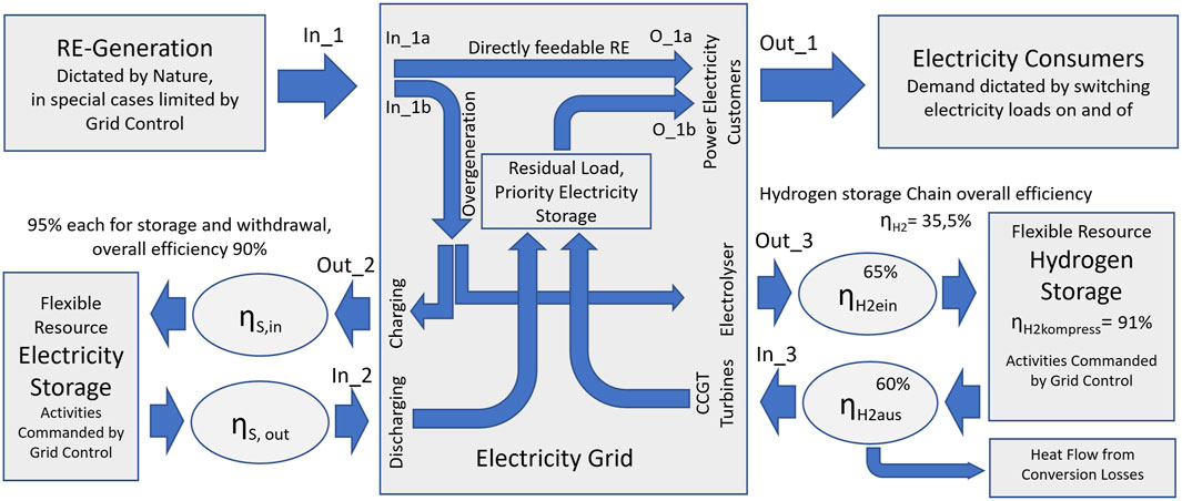
FIGURE 4. Structure of the energy system.

Output Out_1 supplies classic grid consumers, which have demand for private or commercial purposes at times that they determine themselves by switching loads on or off. Battery storage (Out_2) and hydrogen electrolyzer (Out_3) are flexible consumers. Neither can determine their own operating times; they are assigned quantities and times by the grid control system, which must ensure that the sum of all injection and consumption is equal to zero every second.

Since generation and demand are never equal, this condition can only be enforced by using flexible consumers and storage. If the generators are sufficiently sized, the storage systems only need to absorb temporary imbalances over the course of the year; consumer demand and storage losses are met entirely by renewable generation. Since the core of the grid is balanced at any time by the grid control system, this is also true throughout the year. To check if the RE generation is sufficient, we just need to run a year-round simulation and create a storage balance. At the end of the year, there should be slightly more energy in storage than at the beginning of the year to ensure security of supply.

The model shows the ideal situation with no fossil generators and therefore only hydrogen storage. For an intermediate stage, as in the 2030 scenario, a second storage facility for natural gas can be used, but it can only be filled from the outside.

2.3.4 What happens in a simulation run

Looking at our energy model (Figure 4), it is driven by two independently fluctuating and externally determined variables. These are the total output of the RES generators and the electricity demand of the electricity consumers. Both are available as a time series of 1 year consisting of 35,040 (=4*24*365) samples transformed from the reference year to the target scenario according to Section 2.3.2. The task of the network control is to react to these variables and to deploy its resources in such a way that the electricity demand of the customers is matched at all times by exactly the same generation power and the network balance is maintained.

Figure 5 shows the possible constellations of how RE generation (P_RE, green dashed line) and grid load (P_NL, solid black line) can relate to each other.

FIGURE. 5

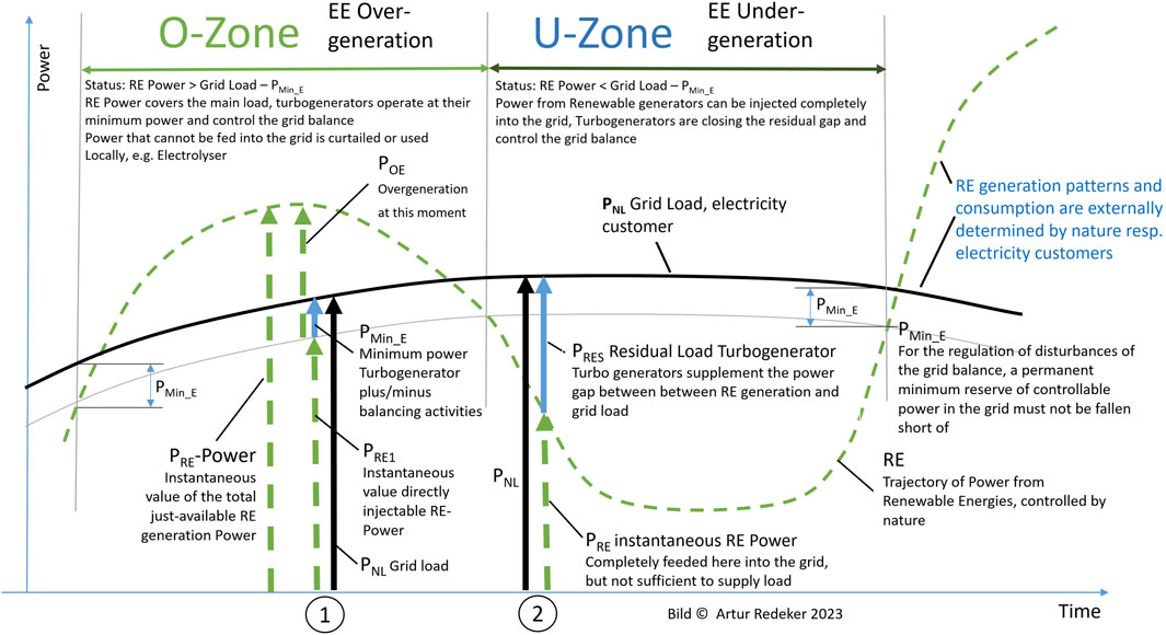
FIGURE. 5. Grid eqilibrium conditions.

A few definitions first:

P_RE: Total RE Power P_RE1: part of RE directly inserted into the Grid

P_{min_E}: Minimum Power of Turbine P_NL: Grid load, consumption Power

P_OE: Overgeneration P_RES, P_Turb: Residual Load, Turbine Power

Here we need to understand the role of P_{min_E}. The only controllable generator resource apart from battery storage is the gas turbine, which would not have to run at high RE output. For grid stability reasons, a minimum of positive and negative regulating power must be available in a power grid at all times. For this reason, we must comply with a constraint that the turbine output never falls below a certain value.

In order to solve the grid control task described above, the simple algorithm described in the following equations is implemented for each sampling.

First, it is clarified according to Eq. 3 whether we are currently in over- or under-generation mode.

O-Zone = true if

$P_{RE}\ge P_{NL}-P_{\min \_E}(3)$

If this is the case, Eq. 4 is used to calculate the directly injectable RE power, Eq. 5 determines the overgeneration and Eq. 6 sets the turbine to minimum power.

If O-Zone:

${\mathrm{P}}_{RE1}={\mathrm{P}}_{NL}–{\mathrm{P}}_{\min \_E}(4)$

${\mathrm{P}}_{OE}={\mathrm{P}}_{RE}–{\mathrm{P}}_{\text{RE}1}(5)$

${\mathrm{P}}_{turb}={\mathrm{P}}_{\min \_E}(6)$

Here the addition of P_RE1 and P_{min_E} is the exact counterweight to the customer Demand P_NL.

In the other case (U-zone), the full renewable electricity can be fed into the grid (Eq. 7) and must be supplemented with residual electricity from the turbine (Eq. 8) in order to meet the electricity customer demand.

If U-Zone

$P_{RE1}=P_{RE}(7)$

$P_{turb}=P_{RES}=P_{NL}-P_{RE}(8)$

The way in which the surplus generation (P_OE) is stored and how the residual power (P_RE) is drawn from the turbine and/or the battery storage is determined by the storage strategy.

Electrical storage systems such as batteries have low losses, but due to high costs they are limited to lower storage capacity. With a gas grid in the background, long storage times and large capacities are possible via hydrogen generation. Unfortunately, the conversions are associated with much higher losses.

A simple but efficient storage strategy is used for our investigation: As soon as excess power occurs and absorption capacity is available in the electrical storage, it is filled with priority; when it is full, hydrogen is produced and stored. In the event of residual power demand, this is taken from the electrical storage system first. Once these are exhausted, electricity will be generated from gas turbines.

On this basis, the storage strategy is applied to each sample, and after all annual slices have been processed, an energy balance is built. Initially, these algorithms were implemented in Excel. Due to the error-prone nature of 30′000 line large and computationally intensive Excel spreadsheets, the algorithms were reimplemented using a simulation tool based on Delphi 10. The purpose of this measure was to verify the results of the Excel calculations and to perform more cross-checks on the integrity of the results.

3 Results

3.1 The scenario 2030

As no significant amounts of electrical storage are expected by 2030, the energy model has been calculated here without such storage. The right-hand side of Table 1 shows an estimate of the possible yields according to the trend scenario from the IAEW study. An increased number of full load hours of 1979 h was assumed for the onshore capacity still to be added by 2030. The IAEW did not show any significant increases for offshore and photovoltaic.

TABLE 1

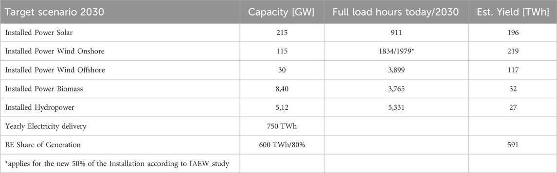
TABLE 1. Targets of the 2030-Scenario and Yields according to historic utilization.

Even in the unlikely event that all RE can be used, a yield of 600 TWh would be required to achieve the target. An installation that produces significant quantities at a high, difficult-to-use output level, but only generates 590 TWh in total per year, must be considered severely undersized.

A full year simulation run that processes the grid balance equations Eq. 3 to Eq. 8 according to the previous chapter of this scenario clearly confirms this with its producer-consumer balance (Figure 6 right). Around 56 TWh of RE generation is a generation surplus that can only be used if flexible consumers are available at the exact time when this energy is generated (case #2). They have to accept very difficult boundary conditions. If you take a closer look at the time course of these 56 TWh, the energy is packaged in short, high power peaks of up to 104 GW.

FIGURE. 6

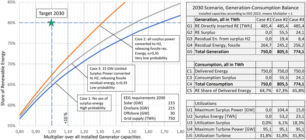
FIGURE. 6. Results of the scenario 2030.

Without their use (case #1), the share of renewable energies in generation is below 65% and is therefore far from the target. Full utilization of these 56 TWh (case 3) would mean that an expensive infrastructure would have to be provided to cope with such a high output, while capacity utilization is extremely low (6%), not economically viable and therefore very unlikely.

Limiting the maximum peak power to 15 GW (Case #3) would improve the degree of excess utilization to 18%, but also discard more than half of it. Hydrogen from electrolysis would leave us about 8.4 TWh to replace fossil residual energy with state-of-the-art efficiencies. The largest electrolysis prototypes (Shell REFHYNE I) with a capacity of 10 MW are more than three orders of magnitude away from 15 GW, making even case #3 by 2030 more than unlikely.

In the simulation, residual energy is generated from turbines with natural gas that is partly replaced by generated hydrogen in the cases #2 + 3. With 750 TWh delivered target work and RW_A as fossil generated Residual Work, the share of renewable energies is calculated as in Eq. 9

$\text{EE}-\text{Ratio}=\left(1-{\text{RW}}_{\mathrm{A}}/750\text{\hspace{0.17em}TWh}\right)*100\%(9)$

As we are so far away from the target with the generation system required by the EEG, the diagram in Figure 6 on the left shows what additional installation of all RE systems would be required to bring us closer to 80%. The x-axis shows a linear multiplier over the capacities of all wind and solar generators, while the ordinate shows the resulting values for cases #1 (bottom line, blue), #2 (top line, red) and #3 (middle line, gray).

Here are three conclusions:

1. The EEG targets are inconsistent because the specified installed capacity for 2030 is not nearly sufficient to supply the required annual energy.

2. If neither the upper nor the middle characteristic curve can be achieved in 2030 due to the unavailability of electrolysis capacity, the future truth is likely to be slightly above the lower blue line. In order to achieve the 80% target by simply not using excess generation, the installed capacity planned for 2030 would have to be exceeded by more than 60%, which is illusory. The key to getting closer to the 80% target lies in the use of surplus energy.

3. The energy yield of the reference year was around 10% below that of an average year, which would have been a small amount closer to the target. According to the IAEW study, even significantly lower yields can be expected within a 10-year period. An industrialized nation should not base its energy planning on the hope that the weather gods will not use their leeway.

Given the current state of the energy transition, it is unlikely that enough energy demand from building heating and electromobility will actually be added to the grid by 2030 to increase annual energy demand to 750 TWh. Missing the transformation targets on the consumption will make it easier to formally achieve the 80% renewable energy target, provided that the development of renewable energy producers is completed on time. Politicians will therefore be very interested in reaching this target. If they are also interested in knowing how much load can be added to today’s 550 TWh annual supply in this case, the simulation system presented here can answer this question: Almost none. This means that with the same weather conditions as in 2021, with all generators operating according to plan, with no further shift of energy from mobility and heating to the grid, and with no further economic growth, we would reach the target of 80% renewable energy in our grid.

Since the failure to meet the targets is already built into the specifications, it appears that the legislators were not sufficiently aware of the consequences of the fluctuating nature of RE generation when drafting the latest EEG amendment.

3.2 Results for the DIW-Scenario (2040+)

3.2.1 Estimation with the help of utilization rates

The second scenario examined here is that of the DIW Berlin study cited above, which was intended as policy advice. It aims to show that Germany can be largely self-sufficient in renewable energy without having to rely on imports that exceed the usual level in the European grid.

The DIW recommends installed capacities for RE generation (Table 2, left blue) and claims that they allow Germany to supply a carbon-free annual electricity volume of 1,070 TWh for a sector-coupled grid, including the production of 139 TWh of hydrogen for processes that are difficult to electrify.

TABLE 2

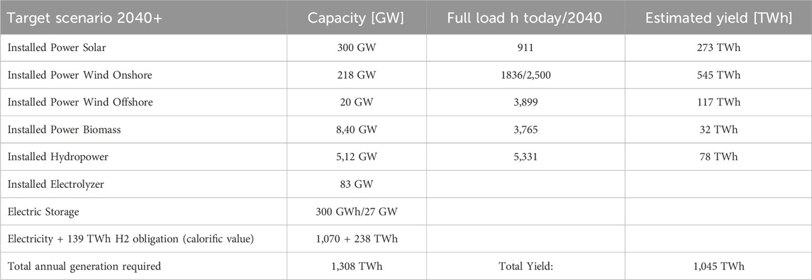
TABLE 2. Targets of the DIW-Scenario and Yields according to expected utilization.

As in the previous scenario evaluation, the right-hand green section of Table 2 shows the expected revenues from utilization levels and the electricity requirements. Even with the assumption of 2,500 full-load hours onshore from the study by a wind power lobby group (Borrmann et al., 2020) which can have no interest in understaking here, the yield calculated via utilization factor is far below requirement. This is true even without an obvious miscalculation, which should be mentioned here. Designation of a gas quantity in electrical units usually means calorific value. Generating this quantity from electricity requires approx. 238 TWh Electricity² instead of 139 TWh.

Since the high deviation suggested a misunderstanding, the author asked DIW for assistance in clarifying the issue. The DIW responded through one of the authors (Kendziorkski, 2022). According to this, they assume that by 2040, all the current wind turbines in Germany will have been replaced by more powerful turbines with higher annual full load hours. Therefore, a value of 3,500 full load hours for onshore wind was assumed for the publication (today 1840 h).

It is difficult to understand what justifies such an assumption. In its answer, the DIW refers to the Global Wind Atlas (globalwindatlas.info) and the EU project OpenEntrance, but in each case without any concrete indication as to how 3,500 full-load hours are to be achieved as an average over the German landmass. When answering such a core question, it is to be expected that the most valid reason is given first. In the DIW response, this is the reference to the IAEW study already cited here (Schwaeppe et al., 2022). It does not support such an assumption at all, apart from the fact that it was published only 1.5 years after the DIW paper. Since wind turbines are largely aerodynamically designed, no major progress can be expected from improved design. According to the Windguard study, the expected increase in efficiency is solely due to the fact that larger turbines are taller and protrude further from the ground boundary layer.

Conclusion: The assumption of 3,500 full load hours on land is far beyond reality. The estimate of 2,500 h made by a lobby group, which has no reason to underestimate, but must also expect to be called to account, is therefore categorized as being in the “cautiously optimistic” range and not corrected here.

In view of the additional challenges posed by significantly higher fluctuations than in the 2030 case, this scenario can already be classified as severely undersupplied.

3.2.2 Simulation results for the DIW scenario

3.2.2.1 The storage balance

The results of an annual simulation of the DIW scenario are shown in Figure 7. The energy model as per Figure 4 is consistently applied here. All excess generation is first stored electrically; when the storage is full, it is electrolysed up to the limit of 83 GW as specified by DIW and then compressed to cavern pressure, the rest is curtailed. Residual power is first generated from electrical storage and then with hydrogen turbines. The right half shows the energy balances of grid generation and consumption as well as the storage balance after both the electrical storage and the hydrogen storage have been restored to their annual starting levels.

FIGURE 7

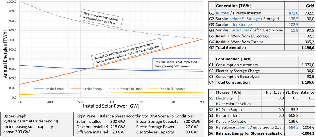
FIGURE 7. Result summary of DIW-Scenario.

In the summary of its publication, aimed at politicians, the DIW states

“A full supply of renewable energies in Germany in the European context is also possible with greater consideration of decentralization and spatial proximity to consumption of generation, without being dependent on imports of hydrogen or other synthetic energy sources.”

Fulfilling this promise made by the authors, requires a positive or at least neutral storage balance.

What we have examined here is an energy system for which almost five times the capacity of today’s solar and wind power generators must be installed compared to the reference year. Furthermore, gas turbine capacity for almost the full grid load of 130 GW must be kept available all year round, but only 15% of it’s capacity is utilized. In addition, 300 GWh of battery storage with a capacity of 27 GW are required and 83 GW of electrolysers, which are utilized at 50%. A screenshot of the simulation display with further detailed information can be found in Supplementary Figure S1 in the Supplementary Material.

In order to be able to generate the desired 1,070 TWh of grid electricity and 139 GW of hydrogen with all these investments, almost the same amount of electrical energy must be feeded in from outside.

When faced with such a result, the first thing to do is to look self-critically for errors in the assumptions and methods used in the investigation. We can look for possible errors, or explain why the result is plausible, or both. The algorithms are disclosed here in the paper and in the Supplementary Material, they are far from complex. To avoid computational errors, they were implemented using two very different software systems. Addinionally, in each 15-min sample, all energy subtotals are checked for violations of the first main theorem, as well as at the energy components of all storage units at the level of the annual balance.

However, errors can also occur due to a incorrect or weak approach. It is certainly debatable whether the assumption of a rigid load curve as it exists today is appropriate, or whether a much higher degree of flexibility in the timing of customer demand cannot be expected in the longer term. Werner Sinn (2017) has looked at the possibilities that immediately come to mind and concluded that we should not expect too much. However, it may be that in 15 years time much more will be possible than we see today, for example, if spatial changes bring processes closer together, making waste heat usable where it is not today. Consumers and energy producers will have to “shake things up” in lengthy optimisation processes, and this will certainly not be achieved by government regulation. We do not know today what can be achieved in the end.

So we are rigorously analysing where the energy losses are coming from and looking for good reasons to explain why the result is plausible.

3.2.2.2 The EE-Power distribution function and its impact on residual work

A first look at the time courses of generation and consumption provides an initial indication. Figure 8 shows the course of the first 4 months; individual days are still clearly recognizable in the temporal resolution. The difference areas below the consumption curve to the red generation curve represent the residual work to be done, the areas above represent surplus. It can be seen with the naked eye that the surplus areas are significantly smaller than the residual areas. For hydrogen storage to lead to a neutral storage balance, the areas above the blue curve would have to be about three times as large due to the conversion losses. This is by no means the case, for the rest of the year either.

FIGURE 8

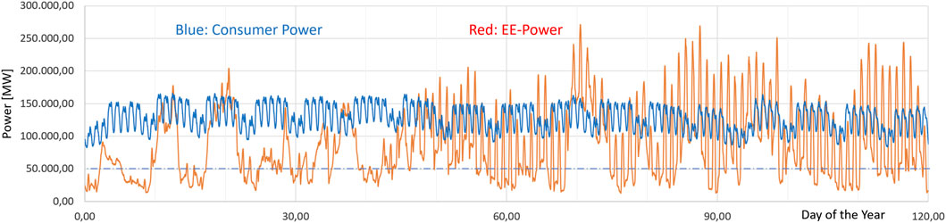
FIGURE 8. DIW-scenario consumer and EE power over the first 120 days of the year.

The comparison with the power curve from the DIW publication provides more information. The generation curve of a week from the DIW paper shown in Figure 1 is described by the authors as the time of lowest RE feed-in in the year. What the DIW graph has in common with this one is the shape of the consumption curve, which shows a similar daily rhythm and supports the assumption of rigid demand. However, it is striking that the instantaneous value of total EE power never falls below 50 GW in a week of lowest generation. In contrast, the natural power curve used here, partly shown in Figure 8, falls below the 50 GW threshold more than 150 times in the course of the year. Histograms in Figure 3, which are all transformed to the DIW target generation, confirm that the total RE output is below the 50 GW threshold for a total 77–117 days in all years.

The DIW graph can only be explained if the RE generation of the calculation models used is based on a different, unrealistic power distribution. This is presumably based on the expectation that if the installed capacity is large enough, the power curve will flatten and the remaining gaps below 50 GW will close. However, there are no good reasons for such an expectation.

Using the example of wind energy, Ahlborn and Schuster (2018) have shown that the added sum signal of independently fluctuating wind generators leads to higher, and not smaller fluctuations than the individual plant. This is similar to the differences in the frequency of occurrence of different numbers of the die, which are felt to even out over many rolls. In reality, the differences become greater and greater as the number of throws increases.

In the case of RE generation, the mere increase in installed capacity in the same region does not even mean the summation of statistically independent but correlated sources. This is not much different than the mere amplification of the same signal, from which no change in dynamics occurs, if the term “dynamics” is understood as the ratio between highest and lowest Power level.

The hope that high installed capacities would close the deeper generation gaps is accompanied by the assumption that the required residual energy would fall sharply with additional generation.

Knowing from chapter 4.2.1 that the system is underserved, we need to test its response to increased generator output. Here we do not have too many options.

In order to realize the expansion of onshore wind turbines alone to the 218 GW already assumed here, around 40,000 turbines will be required, if only large wind turbines with an average output of around 5.5 MW are used. According to Destatis, Germany has an area of 357,000 km²; if you subtract forests, bodies of water, traffic and populated areas, this leaves around 200,000 km². If the 40,000 turbines are distributed evenly over the area, every corner of a grid length of 2.2 km would be occupied by a wind turbine. This is considered to be already beyond social acceptance. A further increase for offshore may be possible, but very likely the 218 GW onshore are already beyond limit. The expansion potential of solar generators is seen by the Ministry of the Environment as 900 GW rooftop + 226 GW for ground-mounted systems. Thus we decide to look at our system’s response to more solar power.

Figure 7 on the left shows us how the important system parameters respond on a successive increase of solar Installation:

- Despite an enormous expansion of solar capacity up to the maximum possible rooftop installation of 900 GW (!), the residual work is completely unimpressed by this. It is only reluctantly and slightly decreasing.

- The amount of energy that can be shifted into the residual gap by electrical storage remains largely constant. Here, either the storage capacity, it’s power or both are limiting.

- Only a small proportion of the additional solar energy is fed directly into the grid. The linear growth of surplus generation indicates that it rolls almost completely off the system and ends up in the electrolyzer and thus in the hydrogen tank. However, even at maximum solar power, it cannot cover the demand that is taken from the storage system by generating the residual work. The deficit remains, but has been reduced from 980 TWh to 610 TWh. Screenshot SM-2 (Supplementary) shows more details of DIW Scenario balance for 900 GW solar.

3.2.2.3 Why residual work is so resistent against increased EE-Power

Two typical observations, which are representative of many situations in summer and winter, make it clear why the residual work with low generation is the main culprit for the poor storage balance and why this has such a high resistance to high installed capacities.

Figure 9 left shows the situation of a so-called tropical night, which we have been experiencing with increasing frequency in Germany in recent years. They occur during typical large-scale high-pressure systems that calm the wind from the Alps to the North Sea. The red solid line is the total RE output, which consists mainly of solar power and very low wind power. The sky was quite cloudy during the day, otherwise the solar peak would be more intense. At night, there is only minor renewable energy power P_RE resulting from from low wind and the almost constant RE types biomass and hydropower. From sunset to sunrise, almost the entire residual load P_Res must be supplied by hydrogen. As a thought experiment, a doubled RE generation capacity is shown here as a dashed red line. It can be seen that even this hardly reduces the residual load in the decisive period. In popular scientific terms: Two times nothing remains nothing. A further increase would only make the solar flanks steeper here, but would only slightly reduce the power-time areas responsible for the residual work.

FIGURE. 9

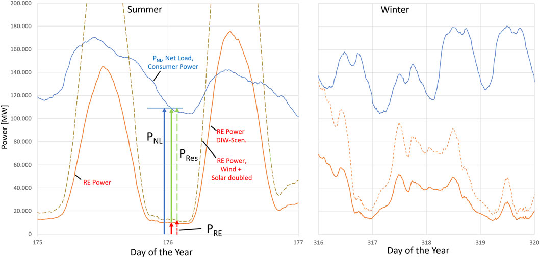
FIGURE. 9. Typical low-RE situation in summer and winter.

The winter situation is not as extreme in the levels, but while the sun is so weak, and stable high pressure weather often lasts for several days, there is also a huge amount of residual work accumulating.

Simply put, it is the large number of short and longer times at which the total power is so low that the residual power is almost independent of higher or lower installed power. The need for residual work, which results from the statistical behavior of the fluctuations, explains and confirms the system behavior observed in the simulation.

In summary, it can be stated that the cause of the poor energy balance results from the combination of two factors.

- Due to the power distribution of natural generation, the residual work required to operate the grid has a hard core that cannot be cracked even by the highest installed capacities

- The poor efficiency of the hydrogen storage chain³

3.2.2.4 Improvement from electric storage applied to solar enhanced scenario

The term “capacity” as a parameter is often used ambiguously in English; in the case of a solar generator or wind turbine, it refers to the “installed power” in multiples of watts. Therefore, it should be specified here that, in the context of storage systems, “storage capacity” refers exclusively to its ability to absorb energy in watt-hours or multiples thereof, while “storage power” refers to the power with which it can be filled or discharged. In order to get away from a situation where two thirds of the storage energy are lost, it makes sense to use electrical storage that has much higher efficiency.

“Politikberatung 167” only discusses the power of storage systems, but makes no mention of their most important attribute: capacity. The maximum power of a storage system determines how much temporal residual power it can replace when it is discharged, or how much excess power it can absorb when it is charged. Power only represents the size of the tank cap, not the volume of the tank, which would correspond to its capacity to hold an amount of energy from which it derives its raison d’être. The DIW only states that a power of 27 GW is required for their integrated scenario and 2 GW for their efficiency scenario. However, without the unfortunately cost-determining ability to absorb a certain amount of electrical energy, storage is pointless. Kendziorki et al. (2021) do not explain why no capacities are mentioned, in another publication (Zerrahn et al., 2018) the partly same authors argue that storage in so-called Residual Load Duration Curve (RLDC) strategies is only considered as a power source/sink. This is true, but storage costs are mainly determined by capacity. When expensive storage replaces expensive hydrogen, it is important to achieve an economic optimum, which is given by a sufficient energy turnover from times of surplus to times of residual load demand. This optimum depends on the capacity, the on-off performance of the storage and the temporal distribution of the fluctuations. In battery storage systems, capacity and power are not really independent design degrees of freedom, they are closely linked by the technology. Limiting an existing on-off power due to a storage strategy is technically straightforward. Expanding capacity is a cost driver, it automatically expands on-off power, ultimately the key to effectiveness and cost is adequate capacity.

In order to determine which capacity the DIW authors use here but do not mention, it can be read from a diagramm of the policy recommendation that is shown here with permission of DIW as Figure 1. In a power-time diagram, area stands for energy (=electrical storage capacity), the capacity of the storage used by DIW can be estimated using the axis labels and a simple measuring grid. The largest measurable battery area is at the edge of the picture, i.e., larger than the part shown, which represents a minimum capacity of about 300 GWh.

The DIW is tacitly presenting politicians here with a storage facility that is about 200 times larger than the largest prototype storage facility known today (which is located at the Vistra “Zero Moss Landing Energy Storage Facility”) in Monterey/USA and has a capacity of 1.6 GWh with an on-off storage Power of 400 MW. Of course, it is basically okay to use something like this in a study of the future. But when, right next to the publication (Göke, 2021), a co-author (Kemfert, 2021) assures politicians that with enough wind and solar generators Germany could be supplied 100% from renewable energies in the shortest possible time (2030) and conceals the fact that this requires the use of technologies of which we do not know today whether they will ever reach an acceptable cost level, this is misleading. Battery storage is fundamentally suitable and scalable, but is still a long way from being competitive in terms of price. Prototypes are only just above the 1 GWh capacity level, i.e. around a factor of 1000 away from future demand. The same applies to electrolysers; pilot installations in Germany are in the 10 MW range, an order of magnitude further away from the 83 GW of the DIW scenario.

For this investigation, typical data for lithium batteries are assumed here. Charging and discharging efficiency, including converter losses, are both 95%. Every TWh of electricity that can be shifted into the residual gap with the help of electrical storage saves almost three TWh of expenditure for balancing the hydrogen storage system.

Storage can only shift existing energy over time. As the DIW scenario is fundamentally undersized, it must first be given additional generation capacity, which, as already shown, is most feasible with solar power. At 900 GW, we have chosen the maximum possible value for rooftop systems. The aim now is to determine how much surplus energy can be shifted into the residual gap by running simulations with modified storage capacity and storage performance.

Figure 10 shows the results. Each data point on the curve represents the reduced residual energy of a full annual cycle after the application of storage. Both axes of the graph have the unit TWh. For each operating point on the storage curve, the ratio of ΔRW/ΔRC indicates the multiple of its own capacity that the storage system can replace in terms of residual energy over the course of a year.

FIGURE.10

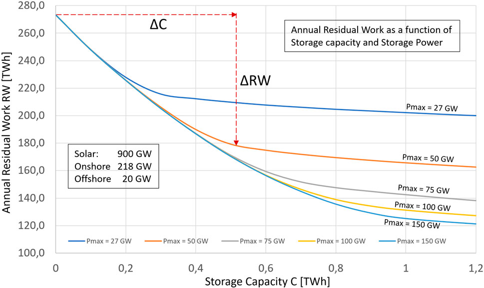
FIGURE.10. Dependency of residual load from Storage capacity and Power.

Just below a capacity of 0.2 TWh, even storage facilities with low charge/discharge power have a slope of around minus 215, i.e., they can shift 215 times their capacity into the residual gap under the conditions of this year. The higher the charge/discharge power, the wider the capacity range in which this ratio is still favourable, before the curve starts to flatten out. At a power of 150 GW and a capacity of 0.8 TWh, the storage can still transport 174 times its capacity, or 139 TWh per year.

If we look at the energy balance of this scenario extended to 900 GW of solar capacity and a storage capacity of 0.8 TWh/150 GW, we still have an annual deficit of 426 TWh. This can be reduced to around 160 GW if we could feed all the surplus into electrolysis, but this would require an insane increase in electrolyser capacity from 83 to 550 GW. For more details on the last two cases, see Supplementary Figures S3, S4.

3.2.2.5 Conditions for an energy neutral configuration

In many engineering disciplines, simulations like this are used to iteratively determine technical target configurations with multivariable influences. Here we iterate such a solution with the remaining degrees of freedom of the DIW model. The aim is not so much to recommend this for implementation. Rather, the aim is to better understand and explain the associated challenges.

With the latest configuration, onshore wind is already exhausted and solar potential also has little room for improvement. Offshore electricity, is less pulsed than solar power and generates a higher yield per installed capacity. So we are taking the expensive route here and increasing offshore from 20 to 50 GW. We leave storage unchanged at 0.8 TWh/150 GW. With a loss of only 18 TWh per year, we would already be close to the target if we still did not have the need of 560 GW of electrolysis capacity (Supplementary Figure S5).

Since RE generators do not have recurring fuel costs, Schill et al. (2018) advocate the tactic of using a sufficiently high installed capacity to release small amounts of energy through “moderate curtailment” of power peaks, thus keeping storage and electrolysis capacity low. We will see that this approach makes sense in principle, but that the orders of magnitude are different from those described by DIW. To achieve a positive storage balance at all, we choose the last option and install a further 300 GW of solar power using all the remaining open space in Germany and a little more, which would give us a positive balance of almost 100 TWh if we could use all the energy (Supplementary Figure S6). Let’s look closer at the temporal distribution of the remaining surplus energy in this configuration before we start cutting back.

The histogram in Figure 11 shows us how the dwell times of the over-generation are distributed across the power classes, which here reach up to almost 800 GW. An almost linear decrease in frequency (= dwell time) can be observed in the upper power range. This should not lead to the misconception that the energy content in the upper power classes is getting lower and lower and that therefore only little energy is lost when these are curtailed. The energy content of a single power band is proportional to the product of frequency, power class and bandwidth. As long as the increase in power class is accompanied by a proportional decrease in frequency, the energy contribution of the power classes remains constant. As can be seen in the right-hand curve in Figure 11, this is the case over a wide range of the power spectrum. It shows the energy sum contained in the power classes up to the abscissa value. The increase therefore remains linear as long as each power class makes the same energy contribution.

FIGURE 11

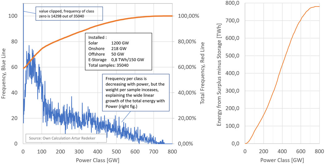
FIGURE 11. Temporal power distribution and cumulative energy of excess generation remaining after electric storage.

Significant curtailment therefore always has a noticeable price. However, curtailment at the level of power P_X does not mean that all peaks P_X are lost, they just remain at P_X. Limiting the output therefore increases the degree of utilization for a connected ressource like an electrolyser.

In our present configuration with a positive balance of 100 TWh, the electrolyser has to process 778 TWh of surplus electricity, which peaks at up to 755 GW. The capacity utilization is therefore a disastrous 12%. If we curtail this for a 250 GW electrolyzer, we end up at +18 TWh and achieve our target of a neutral or positive balance. We lose 223 out of 778 TWh, while the elektrolyser utilization rises to 25% (Supplementary Figure S7).

Table 3 presents a comparison where the DIW policy recommendation and this study differ in the required ressources to produce 1,070 TWh Electricity and 139 calorific TWh of Hydrogen.

TABLE 3

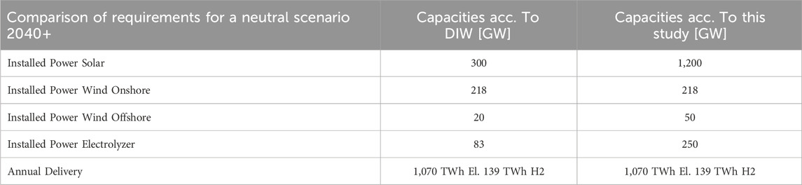
TABLE 3. Comparison of Ressource requirement for an Energy neutral Scenario.

The question is what this has in common with a Pyrrhic victory, given the incredible resources required.

3.2.2.6 Uncertainties of this analysis

The development of the future share of flexible consumption on the electricity demand side has already been mentioned as an uncertainty factor. Energy supply is an important factor in the competitiveness of an economy. Competitive pressures often result in the need for good and regular utilisation of human resources and capital-intensive production facilities. This continues to indicate a considerable inflexibility of demand in terms of time, but the creativity of people should not be underestimated; perhaps there will be good and creative solutions to change this in the future.

The accuracy of the results of this study is also impacted by several other factors. The data files available from the Network Agency originate from the European Network of Transmission System Operators for Electricity (ENTSO-E) and have been corrected several times retrospectively. The changes observed so far for generation data are at the very low end of the range. Slightly larger revisions are observed for the annual installed capacity, with revisions in the range of up to 5%. It is unsatisfactory that there is only one value per year without further information on the time to which it refers, although it is clear that with current growth there must be differences at the beginning and end of the year. As they have an impact on the transformation into the target scenarios, they have been evaluated from Fraunhofer ISE with more precise time information, which allowed to assign a mid-year estimate (see Supplementary Material). The remaining uncertainties are not relevant for the conclusions of this study, in particular because of the insensitivity of the difficult factor “residual work” to installed capacity. In order to facilitate the replication of the results, the data used are listed in detail in the Supplementary Material.

In general, it should be noted that this study assumes that all energy generated can be fed into the grid and delivered to customers at any time without any hindrance to transportation. Existing or future transportation restrictions will affect the results.

The method used here of extrapolating the time course of real generation to future installed capacity may contain deviations if there were temporary curtailments in the reference year due to grid transport problems and therefore reduced feed-in. As these quantities must be remunerated in accordance with the EEG, their magnitude is known. A press release fom ARD (2023) quoted a figure of 5.8 TWh for 2021 with reference to the Ministry of Economic Affairs. Such an error of around 1% of annual generation is within the scope of the uncertainties already present here and also does not call the presented results into question.

4 Summary and discussion

The results from the analysis of the two planning scenarios are summarized here.

- Scenario specifications are inconsistent, generation resources do not meet desired supply.

- The statistical nature of generation is not taken into account.

- It can be clearly shown where the energy deficits occur and what their causes are.

- Residual energy demand is very resistant to increased RE installation and forces turbine capacity at full grid peak load.

- Hydrogen storage is associated with such high losses and induces enormous additional demand for RE generators.

- Appropriate capacity utilization for capital-intensive resources such as electrolysers forces considerable curtailment of generation peaks. The losses induce further demand for RE generators.

- Electric storage systems can only partially replace residual energy from excess generation, but have a long way to go in terms of cost and capacity.

- A CO2-free supply of the consumption specified in the long-term scenario only appears possible if the limits for the installation of RE generators in Germany are fully utilized or even exceeded.

- If, the hydrogen from the unavoidable excess RE generation is hardly able to close the remaining energy gap in the electricity grid, it makes no sense to plan any further hydrogen production in Germany.

Whether 1,070 TWh of electricity and 139 TWh of hydrogen will be able to replace the primary energy demand in Germany beyond 2040 is a question that this paper cannot and does not want to answer. The required expansion of renewable energy plants to cover such a demand with a neutral energy balance is so excessive that it is probably far beyond social acceptance.

If no serious methodological or technical errors can be demonstrated in the study presented here, both scenarios will fall far short of their targets.

It is meanwhile accepted that Germany will become a hydrogen importer. What politics has not yet realized is the fact that achieving the transformation goals in Germany is not so much endangered by delays in the development of planned RE generators, but rather by the fact that the desired goals cannot be achieved in this way. Sooner or later, this will force a change in strategy, in which the fixed costs of a poorly utilized but very complex parallel infrastructure of RE generators, hydrogen turbines, storage facilities and greatly expanded transport networks for electricity and hydrogen will replace today’s recurring fuel costs. The study presented here provides a basis for estimating some of these costs.

Data availability statement

The raw data supporting the conclusion of this article will be made available by the authors, without undue reservation.

Author contributions

The authorship and responsibility for all parts of this publication lies with AR.

Conflict of interest

Author AR was employed by arConsulting.

Publisher’s note

All claims expressed in this article are solely those of the authors and do not necessarily represent those of their affiliated organizations, or those of the publisher, the editors and the reviewers. Any product that may be evaluated in this article, or claim that may be made by its manufacturer, is not guaranteed or endorsed by the publisher.

Supplementary material

The Supplementary Material for this article can be found online at: https://www.frontiersin.org/articles/10.3389/fenrg.2024.1240114/full#supplementary-material

Supplementary Data Sheet 1 | CSV.

Supplementary Data Sheet 2 | CSV. Generation and consumption raw data file Germany 2021 from SMARD Portal of Bundesnetzagentur.

Supplementary Data Sheet 3 | A detailed description of the transformation process from reference year raw data to target scenario. 7 Simulation result screenshots with comments.

Supplementary Data Sheet 4 | A description of the data source and the determination of the installed capacities for the reference year.

Supplementary Table 1 | Installed capacities of the reference year as reported from the Bundesnetzagentur.

Supplementary Table 2 | Installed capacities of the reference year as reported from the Bundesnetzagentur.

Supplementary Figure 1 | More detailed Screenshots from the Scenario simulations as decribed Data Sheet3.pdf.

Supplementary Figure 2 | More detailed Screenshots from the Scenario simulations as decribed Data Sheet3.pdf.

Supplementary Figure 3 | More detailed Screenshots from the Scenario simulations as decribed Data Sheet3.pdf.

Supplementary Figure 4 | More detailed Screenshots from the Scenario simulations as decribed Data Sheet3.pdf.

Supplementary Figure 5 | More detailed Screenshots from the Scenario simulations as decribed Data Sheet3.pdf.

Supplementary Figure 6 | More detailed Screenshots from the Scenario simulations as decribed Data Sheet3.pdf.

Supplementary Figure 7 | More detailed Screenshots from the Scenario simulations as decribed Data Sheet3.pdf.

Footnotes

¹The identification of the Installed capacities of the reference year is not trivial in a fast growing setup of generators. The source of the information and the detemined values are avilable in a document of the Supplementary Material.

²According to the current state of the art, fluctuating generation requires PEM electrolysis, best efficiency approx. 65%, compression to cavern pressure takes place with 91% efficiency, so that 139/0.65/0.91 = 238 TWh have to be used.

³Detailed efficiency assumptions can be found in the Supplementary Material.

References

Ahlborn, D. (2015). Glättung der Windeinspeisung durch Ausbau der Windkraft. Energiewirtschaftliche Tagesfr. 65. 37–39.

Google Scholar

Ahlborn, D. (2023). Nutzung überschüssiger Wind-und Solarenergie durch Power-toX Konzepte. Autorenbeitrag in „Generationenprojekt Energiewende“. Norderstedt: Herausgeber Herbert Niederhausen. Available at: https://d-nb.info/1297505700.

Google Scholar

Ahlborn, D., and Schuster, R. (2018). Volatilität und Stochastik der Windstromerzeugung in Deutschland und Europa. World Min. Issue 70 (2), 120–125.

Google Scholar

ARD (2023). Rekord an nicht eingespeistem Strom. Tagesschaumeldung vom 12.12. Available at: https://www.tagesschau.de/wirtschaft/energieversorger-strom-entschaedigung-101.html.

Google Scholar

Ausfelder, J. (2017). Sektorkopplung – untersuchungen und Überlegungen zur Entwicklung eines integrierten Energiesystems. Schriftenreihe Energiesysteme der Zukunft, München, Available at: www.leopoldina.org, www.acatech.de,www.akademieunion.de, http://dnb.d.d-nb.de

Google Scholar

BMJ (2023). Erneuerbare-Energien-Gesetz vom 21. Juli 2014 (BGBl. I S. 1066), das zuletzt durch Artikel 4 des Gesetzes vom 26. Juli 2023 (BGBl. 2023 I Nr. 202) geändert worden ist. Bundesministerium für Justiz. Available at: https://www.gesetze-im-internet.de/eeg_2014/EEG_2023.pdf.

Google Scholar

Borrmann, R., Rehfeld, K., and Kruse, D. (2020). Volllaststunden von Windenergieanlagen an Land. Deutsche Windguard under a contract from Bundesverband Windenergie e.V. Berlin and Landesverband Erneuerbare Energien e.V. Düsseldorf. Project Nr. VW20082, Report Nr. SP20004A2. Available at: https://www.windguard.de/veroeffentlichungen.html?file=files/cto_layout/img/unternehmen/veroeffentlichungen/2020/Volllaststunden%20von%20Windenergieanlagen%20an%20Land%202020.pdf.

Google Scholar

Bowden, G. J., Barker, P. R., Shestopal, V. O., Twidell, J. W., et al. (1983). The Weibull distribution function and wind power statistics. Wind Eng. 7 (2), 85–98. Available at: https://www.jstor.org/stable/43749036.

Google Scholar

Burger, B. (2022). Nettostromerzeugung in Deutschland 2021: erneuerbare Energien witterungsbedingt schwächer. Institut für Solare Energiesysteme, Freiburg. 3. Available at: https://www.energy-charts.info/downloads/Stromerzeugung_2021.pdf.

Google Scholar

Göke, L. (2021). AnyMOD.jl A Julia package for creating energy system models. TU Berlin, FG Wirtschafts-und Infrastrukturpolitik (WIP). https://depositonce.tu-berlin.de/items/538c45a8-d754-429f-9a09-13b3961db992.

Google Scholar

Göke, L., Claudia, K., and Mario, K. (2021). 100 Prozent erneuerbare Energien für Deutschland: koordinierte Ausbauplanung notwendig. Dtsch. Inst. für Wirtsch. (DIW) 88 (29/30), 507–513. Available at: https://www.diw.de/de/diw_01.c.821876.de/publikationen/wochenberichte/2021_29/heft.html.

Google Scholar

Kemfert, C. (2021). Vollversorgung mit erneuerbaren Energien ist möglich und sicher: Deutsches Institut für Wirtschaftsforschung, Berlin Interview im DIW Wochenbericht 29+30.

Google Scholar

Kendziorski, M. (2022). Deutsches Institut für Wirtschaft, Berlin. Personal communication, answering a question to the. Berlin: German Institute for Economic Affairs.

Google Scholar

Kendziorski, M., et al. (2021). Politikberatung kompakt 167, 100% erneuerbare Energie für Deutschland unter besonderer Berücksichtigung von Dezentralität und räumlicher Verbrauchsnähe – Potenziale, Szenarien und Auswirkungen auf Netzinfrastrukturen. Berlin: Deutsches Institut für Wirtschaftsforschung (DIW). ISBN 978-3-946417-58-3. Available at: https://www.diw.de/documents/publikationen/73/diw_01.c.816979.de/diwkompakt_2021-167.pdf.

Google Scholar

Philip, S., et al. (2020). Wege zu einem klimaneutralen Energiesystem-Die deutsche Energiewende im Kontext gesellschaftlicher Verhaltensweisen. Freiburg, Germany: Fraunhofer-Institut für Solare Energiesysteme ISE.

Google Scholar

Schill, W.-P., Zerrahn, A., and Kemfert, C. (2018). Die Energiewende wird nicht an Stromspeichern scheitern. Berlin: Deutsches Institut für Wirtschaft. DIW aktuell 11-2018. ISSN 2567-3971. Available at: https://www.diw.de/documents/publikationen/73/diw_01.c.591369.de/diw_aktuell_11.pdf.

Google Scholar

Schwaeppe, H., Carlo, S., Walter, J. D., Lambriex, J. D., Claire, M. A., et al. (2022). Mittelfristprognose zur deutschlandweiten Stromerzeugung aus EEG-Anlagen für die Kalenderjahre 2023 bis 2027. RWTH Aachen, Institut für Elektrischen Anlagen und Netze, Digitalisierung und Energiewirtschaft (IAEW) on behalf of TenneT TSO GmbH. Aachen. Available at: https://www.netztransparenz.de/xspproxy/api/staticfiles/ntp-relaunch/dokumente/erneuerbare%20energien%20und%20umlagen/eeg-umlage/mittelfristprognosen/mittelfristprognose-2023-2027/2022-10-14_endbericht_iaew.pdf.

Google Scholar

Sinn, H.-W. (2017). Buffering volatility: a study on the limits of Germany's energy revolution. Eur. Econ. Rev. 99, 130–150. Compare also the presentation „Wie viel Zappelstrom verträgt das Netz? Bemerkungen zur deutschen Energiewende“ in the frame of Münchner Seminare an the Ludwig-Maximilians-Universität München, 18. Dezember 2017 (online available). doi:10.1016/j.euroecorev.2017.05.007

CrossRef Full Text | Google Scholar

SMARD (2023). Marktdaten Stromnetz Öffentliche ErzeugungBundesnetzagentur für Elektrizität, Gas, Telekommunikation, Post und Eisenbahnen. Available at: https://www.smard.de/home/downloadcenter/download-marktdaten/.

Google Scholar

Stevens, M. J. M., and Smulders, P. T. (1979). The estimation of the parameters of the Weibull wind speed distribution for wind energy utilization purposes. Wind Eng. 3 (2), 132–145. Available at: https://www.jstor.org/stable/43749134.

Google Scholar

Zerrahn, A., Schill, W.-P., and Kemfert, C. (2018). On the economics of Electrical Storage for variable renewable energy sources. Eur. Econ. Rev. 108, 259–279. doi:10.1016/j.euroecorev.2018.07.004

CrossRef Full Text | Google Scholar