Optimal control of renewable energy communities with controllable assets

Introduction: The control of Renewable Energy Communities (REC) with controllable assets (e.g., batteries) can be formalised as an optimal control problem. This paper proposes a generic formulation for such a problem whereby the electricity generated by the community members is redistributed using repartition keys. These keys represent the fraction of the surplus of local electricity production (i.e., electricity generated within the community but not consumed by any community member) to be allocated to each community member. This formalisation enables us to jointly optimise the controllable assets and the repartition keys, minimising the combined total value of the electricity bills of the members.

Methods: To perform this optimisation, we propose two algorithms aimed at solving an optimal open-loop control problem in a receding horizon fashion. Moreover, we also propose another approximated algorithm which only optimises the controllable assets (as opposed to optimising both controllable assets and repartition keys). We test these algorithms on Renewable Energy Communities control problems constructed from synthetic data, inspired from a real-life case of REC.

Results: Our results show that the combined total value of the electricity bills of the members is greatly reduced when simultaneously optimising the controllable assets and the repartition keys (i.e., the first two algorithms proposed).

Discussion: These findings strongly advocate the need for algorithms that adopt a more holistic standpoint when it comes to controlling energy systems such as renewable energy communities, co-optimising or jointly optimising them from both a traditional (very granular) control standpoint and a larger economic perspective.

1 Introduction

Decarbonising the electricity generation sector is currently one of the primary goals towards curbing anthropogenic emissions of greenhouse gases. To that end, various energy policies around the world have set out to provide guidelines and pathways toward achieving this goal (Code de l’énergie Français, 2017; European Union, 2018; Service public de Wallonie, 2019; Torabi Moghadam et al., 2020). A key enabler of decarbonisation is the decentralisation of power generation, which now enables the electricity to be generated closer to where it is consumed. The production assets are, in this case, typically small, such as solar photovoltaic (PV) panels, and are directly connected to the distribution networks. However, this decentralisation does not come without challenges. Several technical as well as regulatory challenges emerge when a significant proportion of the electricity consumed by the end customer is produced near or at the consumption centres (e.g., by prosumers) as addressed by (Manuel de Villena et al., 2021). These problems exist due to, among other reasons, the lack of regulatory frameworks defining how the electricity can be traded in decentralised settings. In this regard, various trading alternatives have been studied and described in existing literature, the most relevant ones based on peer-to-peer (P2P) electricity trading and on trading via a centralised entity. Concerning the first one (P2P trading), a substantial amount of research already exists, including these two literature reviews (Tushar et al., 2018; Sousa et al., 2019), which encapsulate the existing works in the context of these types of exchange. The former review deals with P2P mechanisms using game-theoretical approaches, whilst the latter provides a motivation for the existence of these markets, identifying several challenges, market designs, and potential future developments in this field. As for trading through a central entity, the literature is less abundant and focuses mainly on aggregator or retailer models [see for instance (Mathieu et al., 2019)]. Over the last few years though, a new concept has entered the arena: the Renewable Energy Communities (RECs). Some literature (Moret and Pinson, 2018; Cornélusse et al., 2019; Manuel de Villena et al., 2020a) exists on how the control of energy consumption and production of consumers inside a REC can be computed; however, the lack of adequate regulation has made it difficult to apply any of those mechanisms in practice.

In an effort to provide a framework to boost these new decentralised markets, in the latest Energy Package, the European Commission has embraced the concept of a REC and has introduced, for the first time, a formal definition of these communities along with some basic working principles (European Union, 2018). According to this definition, RECs constitute a type of consumer-centric electricity market comprised of consumers, prosumers, and generation and storage assets that may be shared by all or a subset of the REC members. In this context, electricity surplus generated from prosumers and reinjected into the network can be allocated to the community and shared among the REC members. Thus, a fraction of the total electricity surplus can be allocated to each REC member at a lower price than the retail one. In this paper, this surplus is denoted as local production surplus. As per European regulation, RECs are managed by a central entity: the energy community manager (ECM), whose responsibilities include ensuring the adequate functioning of the REC. Although the rules of participation in a REC are precisely outlined in this European regulation¹, there is no provision dictating how to share the local production surplus within the REC. Furthermore, to date and to the best of our knowledge, little or no research has addressed the issue of performing the control of flexible assets such as storage devices within a REC context, which often modifies this local production surplus within the REC, as further explained in Section 2.

To fill this gap, the main contribution of this paper consists of providing a new methodology to simultaneously control, in an optimal manner, the generation and storage devices of RECs with the allocation of the local production surplus to the REC members. Our methodology provides a generic formulation of the decision process associated with the control of RECs, one sufficiently flexible to work with any composition of a REC and to the specific rules applying to it. This decision process, for which the formulation is detailed in Section 3, describes the dynamics of the controllable assets of each member (e.g., batteries), as well as the distribution of local production surplus among the REC members. To that end, it exploits the concept of repartition keys, which are introduced in (Manuel de Villena et al., 2020b). Repartition keys represent the fraction of the total production surplus which is allocated to each REC member—there is one key per member and time-step of the simulation. These keys are computed in the framework of our decision process. Along with the decision process, we propose two algorithms, described in Section 4, which directly exploit the specification of the decision process itself to jointly optimise the control of the controllable assets and the repartition keys in a finite time window. The goal of these algorithms is to jointly minimise the cost related to the controllable assets and the combined total value of the electricity bills of the members that is dependent on the repartition keys (e.g., the combined total value of the electricity bills of the members after allocating the local production surplus to the REC members). Then, a test case is provided in Section 5, where a REC is constructed from synthetic data—the two algorithms described in the previous section are here benchmarked against a third one, that does not optimise the repartition keys, illustrating the relevance of jointly optimising the repartition keys when controlling RECs. Finally, Section 6 concludes this paper.

1.1 Gap targeted and summary of the hypotheses

In this paper, we target a centralised optimisation of the REC electricity bill where we simultaneously command the controllable assets and periodically re-allocate the electricity production surplus of the whole REC. The main hypotheses are as follows.

• The controllable assets of each member are managed at a fixed time rate (e.g., 15 min),

• The dynamics and the operational costs of the controllable assets of each member are known at runtime and assumed, in the experiments of this paper, to be linear,

• Any electricity production surplus of any member can be either redistributed to net consumers inside the REC or sold to the retailer,

• The network topology is not taken into account.

2 Related work

Although the exact rules defining how to exploit and control RECs are still “a work in progress,” as seen in (European Union, 2018; Heaslip et al., 2016; Reijnders et al., 2020; Code de l’énergie Français, 2017; Service public de Wallonie, 2019) research into this topic is already gathering momentum. In (Ciocia et al., 2020), the authors propose a sizing and simulation optimisation framework of a microgrid composed of nanogrids, which is a structure similar to RECs, which follows the Italian market framework. However, this is not addressed as a control problem since the optimisation stage is directly performed with the full history of production and consumption of each member of this microgrid. The literature on these control problems is, by and large, scarce, and typically focuses on single-entity problems where a unique agent (i.e., a single end customer such as a microgrid) is optimised with respect to a specific objective, usually a cost minimisation. In this regard, model predictive control approaches, based on mixed integer linear programming (MILP) or dynamic programming (DP), have been used to optimise the control of microgrids, which can be seen as a particular case of RECs with a single member. In (Parisio and Glielmo, 2011), the authors present an MILP as a solution to perform online planning in a microgrid with the goal of minimising the sum of the operational costs related to electricity exchanges with the main network and to the usage of complex devices (e.g., an energy generator with start-up and shut-down commands). Similarly, in (Francois et al., 2016), linear programming techniques are employed to optimise the control of microgrids by balancing the usage of short-term and long-term storage systems in order to minimise the levelised cost of electricity generated by the microgrid control. In (Hooshmand et al., 2012) the authors propose an algorithm that combines dynamic programming and empirical mean of the objective function to control a microgrid under stochastic scenarios of wind turbine production so as to maximise the local energy consumption. In (Cominesi et al., 2017), the authors propose a bilevel optimisation scheme, in a receding time horizon to control a microgrid comprised of a battery, a microturbine, a PV system, and a load. In their work, an optimal daily planning of each controllable component of the microgrid is computed at a time scale of 15 min. Then, a lower-level controller adjusts the control of the microgrid to be as close as the optimal daily plan as possible while respecting the real-time operational constraints. The optimal control of microgrids can be achieved by adopting other techniques, like reinforcement learning (RL) algorithms, which often do not require an assumption relating to the knowledge of the dynamics of the microgrids. In (Tomin et al., 2019), the authors propose to train deep neural networks with RL, specifically with the Q-Learning algorithm (Sutton and Barto, 2018) by exploiting historical data of production and consumption in order to sample control trajectories. Another work using RL, (Nakabi and Toivanen, 2020), benchmarks several deep reinforcement learning algorithms against a microgrid with flexible demand. In (Boukas et al., 2018), the authors propose using Deep Q-Learning to construct a policy that controls a microgrid which places orders in a continuous real-time market while taking into account operational constraints.

The decision processes relating to the control of multi-entity problems, such as the REC, are only covered to a very limited extent by the existing literature. For instance, in (Zhou et al., 2019) the authors adapt the Q-learning algorithm to train an autonomous centralised controller with the objective of minimising the combined total value of the electricity bills within a REC composed of buildings (members) that are equipped with batteries and PV panels. In (Prasad and Dusparic, 2019), a multi-agent deep reinforcement learning algorithm, previously developed in (François-Lavet et al., 2018), is employed to train each member of the REC to cooperate in order to minimise the volume of the energy imported from the main network, that is, the proportion of the REC consumption that is not covered by local generation.

3 Decision process associated with renewable energy communities

This section explains in detail the modelling framework proposed in our work, formalising the decision process associated with RECs. This decision process aims to control the dynamics of the electricity consumption and production of the REC members, as well as the electricity exchanges between them. Each REC member is characterised by i) a non-controllable electricity consumption, ii) a non-controllable electricity production (when it exists) with e.g., PV panels or wind turbines, and iii) a controllable electricity consumption/production (when it exists) with devices such as flexible loads, batteries or hydrogen tanks equipped with fuel cells and electrolysers. Periodically (e.g., each month), REC members are billed for their electricity consumption depending on their metered consumption/production. According to the last European regulation (European Union, 2018), the electricity surplus of a REC member can either be sold to other REC members or can be injected into the main grid via sales to the retailer. On the other hand, the energy consumption needs of REC members may be covered first by their own energy production (if they are prosumers), with the surplus of other REC members via the local REC market, or through a traditional retailer contract. In the context of RECs as described in (European Union, 2018), the ECM of the REC is in charge of distributing the local electricity surplus among the REC members as required. This allocation of the local production surplus can be performed according to different objectives such as the minimisation of the total combined value of the individual REC members’ electricity bills. To that end, we introduce a methodology of local production surplus allocation based on a sequential decision-making optimisation framework. This methodology is based on repartition keys, as described in (Manuel de Villena et al., 2020b). For each member, a repartition key is defined by two values: the first one, namely the export key, determines the fraction of each member’s own local production surplus to be sold in the internal market of the REC, whereas the second one, the import key, determines the fraction of the total local production surplus to be allocated to each member. An illustration of the REC design used in our decision process can be found in Figure 1.

FIGURE 1

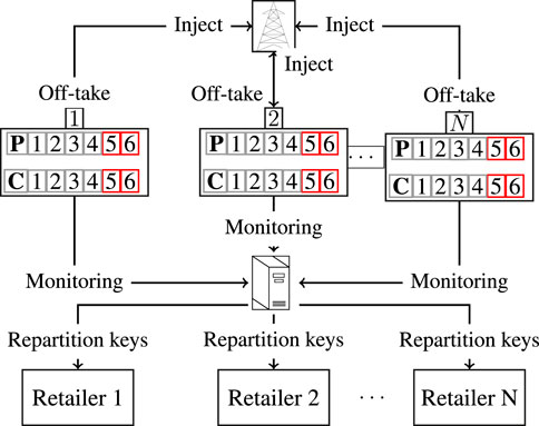
FIGURE 1. Illustration of a REC. Each member $i\in \left\{1,\dots ,N\right\}$ is associated with a specific consumption meter (C) and a production meter (P). At each discrete time step t, these meters are incremented by the energy consumption and production of each member during the time interval] t, t + 1], respectively. These meters are monitored at the end of each metering period by an energy management system (EMS). The EMS can modulate the controllable assets. It also computes optimal repartition keys with the values monitored from all the meters of the REC members and send them to their respective retailers. Retailers periodically (e.g., monthly) compute the electricity bills of each REC members based on the repartition keys and sends them to their respective customers.

3.1 Mathematical formulation of the decision process

The decision process introduced previously can be formalised as a discrete-time dynamical system with a finite time horizon T. Within this dynamical system denoted by $\mathcal{D}$, we can identify the state, action, and exogenous spaces of the dynamical system.

• $\mathcal{S}$ denotes its state space and gathers all possible states of the system.

• $\mathcal{U}$ denotes its action space and comprises the actions that steer the state transitions from one step to the next;

• Ξ denotes its exogenous space and is composed of the exogenous values with non-observable dynamics to which dynamical systems associated with RECs are typically subject (e.g., PV panel production).

With these spaces, we can define the dynamics, denoted f(s, u, e), as the transition from a state-action-exogenous triplet $(s,u,e)\in \mathcal{S}\times \mathcal{U}\times \mathrm{\Xi }$ to another state $s^{\prime }\in \mathcal{S}$. This decision process necessitates information about the REC members, which are encapsulated in the set $\mathcal{I}=\left\{1,\dots ,I\right\}$ with $I\in {\mathbb{N}}^{+}$, where $i\in \mathcal{I}$ denotes a REC member.

3.1.1 Discretisation of the time horizon

The time horizon constituting the dynamical system is split into discrete time steps 0, …, t, …, T − 1. We assume a constant duration equals to Δ_C (e.g., 15 min) for all time intervals $\left]\mathrm{0,1}\right],\dots ,\left]T-2,T-1\right]$. We define such a time interval as a control period. We also define a metering period as the interval $\left]t,t+{\mathrm{\Delta }}_M\right]$ when t mod  Δ_M = 0, where ${\mathrm{\Delta }}_M\in {\mathbb{N}}^{+}$. We assume that control actions are applied to the controllable assets at each discrete time step t and that repartition keys are computed every Δ_M discrete time steps. We further assume that the discrete time step T − 1 always coincides with the end of a metering period (i.e., that T − 1 mod Δ_M = (Δ_M − 1)) and that at each discrete time step t, the consumption and the production of each member, which is measured during the control period $\left]t,t+1\right]$, is added to the present consumption and production of the metering period to which the discrete time step t belongs. Figure 2 illustrates several features of this time discretisation process.

FIGURE 2

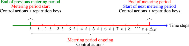
FIGURE 2. Illustration of the time discretization strategy of the decision process described in the problem statement starting from a given time step t and ending at t + Δ_M, where t mod Δ_M = 0. These two discrete time steps both corresponds to the end of a metering period.

3.1.2 State space

Every state $s\in \mathcal{S}$ comprises information for each REC member $i\in \mathcal{I}$ concerning i) the controllable assets (e.g., state of charge of the battery) represented by $s_i^c$; ii) the electricity consumed from the grid during a metering period, represented by $s_i^{e_{-}}$; iii) the electricity produced that is injected into the grid during a metering period, represented by $s_i^{e_{+}}$, and iv) the number of discrete time steps elapsed in the present metering period, represented by s^τ. For compactness, let $s^c=\left(s_1^c,\dots ,s_I^c\right)$, $s^{e_{-}}=\left(s_1^{e_{-}},\dots ,s_I^{e_{-}}\right)$, and $s^{e_{+}}=\left(s_1^{e_{+}},\dots ,s_I^{e_{+}}\right)$. We denote as $s_t=(s_t^c,s_t^{\tau },s_t^{e_{-}},s_t^{e_{+}})$ the state of the dynamical system at a given discrete time step t.

3.1.3 Action space

Every action $u\in \mathcal{U}$ contains i) the actions that can be applied to the controllable assets of each member $i\in \mathcal{I}$, represented by $u_i^c$, ii) the export key vector $u^{k_{+}}$ of size I and iii) the import key vector $u^{k_{-}}$ of size I. The export key determines the fraction of the electricity production surplus of each REC member to be reallocated to other members. The import key determines the fraction of the local electricity surplus to be reallocated to each REC members. For compactness, let $u^c=\left(u_1^c,\dots ,u_I^c\right)$, $u^c=\left(u_1^{k_{-}},\dots ,u_I^{k_{-}}\right)$ and $u^{k_{+}}=\left(u_1^{k_{+}},\dots ,u_I^{k_{+}}\right)$. We denote as $u_t=\left(u_t^c,u_t^{k_{+}},u_t^{k_{-}}\right)$ the action taken from the state s_t of the dynamical system at a given discrete time step t.

3.1.4 Exogenous space

Every exogenous variable e ∈ Ξ contains, for all members $i\in \mathcal{I}$, i) a vector of buying prices $e_i^b$ associated with member i (e.g., retail price); ii) a vector of selling prices $e_i^s$ (e.g., selling price to retailer) associated with member $i\in \mathcal{I}$, and iii) other exogenous variables $e_i^o$ associated with member $i\in \mathcal{I}$ of the community (e.g., PV production). For compactness, we can define these vectors as $e^b=\left(e_1^b,\dots ,e_I^b\right)$, $e^s=\left(e_1^s,\dots ,e_I^s\right)$, and $e^o=\left(e_1^o,\dots ,e_I^o\right)$. We denote as $e_t=(e_{i,t}^b,e_{i,t}^s,e_{i,t}^o)$ the value of the exogenous variable at a given discrete time step t. We assume, for all metering periods ]t, t + Δ_M] where t mod Δ_M = 0, that $e_{i,t}^b=e_{i,t+1}^b=\dots =e_{i,t+{\mathrm{\Delta }}_M}^b$ and $e_{i,t}^s=e_{i,t+1}^s=\dots =e_{i,t+{\mathrm{\Delta }}_M}^s$.

3.1.5 Local production surplus

The local production surplus to be shared among the REC members at the end of a metering period is denoted by Φ and defined as follows:

$\mathrm{\Phi }=\sum _{i\in \mathcal{I}}{u}_i^{k_{+}}{s}_i^{e_{+}}.(1)$

The fraction of this local production surplus allocated to member i is defined by $u_i^{k_{-}}\mathrm{\Phi }$. From these definitions, for all member $i\in \mathcal{I}$, the electricity consumption not covered by local production is $s_i^{e_{-}}-u_i^{k_{-}}\mathrm{\Phi }$. Similarly, the production exported to the main utility grid at the end of a metering period is $(1-u_i^{k_{+}})s_i^{e_{+}}$.

3.1.6 Constraints on the controllable assets actions and on the repartition keys

We assume that the set of admissible actions that can be taken given the current state and the current exogenous variable is given by the mapping $U:\mathcal{S}\times \mathrm{\Xi }\to \mathcal{P}(\mathcal{U})$². While the constraints on the controllable assets are provided at runtime, the constraints on the repartition keys are defined as follows.

3.1.6.1 At the end of a metering period

The repartition keys are set to values between 0 and 1. The amount of the electricity production surplus of the REC imported by a member cannot exceed its consumption. The sum of the import keys among the members is equal to 1. Finally.

3.1.6.2 At others discrete time steps

The only value that can be set for the repartition keys is ∅, i.e., the repartition keys are not defined at these discrete time steps.

The equation below summarises the above-mentioned constraint:

$U\left(s,e\right)\subseteq \left\{\begin{array}{cc}\hfill & \left\{\left[u^c,\varnothing ,\varnothing \right]\in \mathcal{U}\right\}\mathbf{i}\mathbf{f}{s}_t^{\tau }\ne {\mathrm{\Delta }}_M,\mathbf{o}\mathbf{t}\mathbf{h}\mathbf{e}\mathbf{r}\mathbf{w}\mathbf{i}\mathbf{s}\mathbf{e}\hfill \\ \hfill & \left\{\left.\left[u^c,u^{k_{+}},u^{k_{-}}\right]\in \mathcal{U}\right|\left\{\begin{array}{cc}\hfill & u_i^{k_{+}},u_i^{k_{-}}\in \left[\mathrm{0,1}\right]\mathbf{a}\mathbf{n}\mathbf{d}\hfill \\ \hfill & \sum _{i\in I}{u^{k_{-}}}_i=1\mathbf{a}\mathbf{n}\mathbf{d}\hfill \\ \hfill & u_i^{k_{-}}\mathrm{\Phi }⩽s_i^{e_{-}}\hfill \end{array}\right\}\forall i\in \mathcal{I},\forall \left(s,e\right)\in \mathcal{S}\times \mathrm{\Xi }.\right\}\hfill \end{array}\right.(2)$

3.1.7 Net electricity consumption and production during a control period

The net electricity production or consumption is the amount of power injected to or withdrawn from the grid during a given control period, and are denoted by $l_{i,t}^{+}\in {\mathbb{R}}^{+}$ and $l_{i,t}^{-}\in {\mathbb{R}}^{+}$, respectively. These values may be the realisation of any unknown, complex dynamics and may depend, among others, on the control actions $u_{i,t}^c$, for all $i\in \mathcal{I}$. Later in this paper, we will assume that at each discrete time step t, the pair $(l_{i,t}^{+},l_{i,t}^{-})$ is the result of a known function of the state $s_{i,t}^c$, action $u_{i,t}^c$ and exogenous variable $e_{i,t}^o$ for all $i\in \mathcal{I}$.

3.1.8 Transition dynamics

We assume the following known discrete-time transition dynamics for the state space for all $t\in \mathbb{N}$.

3.1.8.1 Controllable assets dynamics

The transition dynamics of the controllable assets of the members, known at runtime, are defined as follows:

$s_{i,t+1}^c=f_i^c\left(s_{i,t}^c,u_{i,t}^c,e_{i,t}^o\right)|s_{i,0}^c=S_{i,0}^c,\forall i\in \mathcal{I},(3)$

where $S_{i,0}^c$ is the initial state value of $s_i^c$.

3.1.8.2 Metering period counter dynamics

The transition dynamics of the counter of the remaining discrete time steps in the current metering period is defined as follows:

$s_{t+1}^{\tau }=\left.\left\{\begin{array}{c}{s}_t^{\tau }+1\mathbf{i}\mathbf{f}{s}_t^{\tau }<{\mathrm{\Delta }}_M\hfill \\ 0\mathbf{o}\mathbf{t}\mathbf{h}\mathbf{e}\mathbf{r}\mathbf{w}\mathbf{i}\mathbf{s}\mathbf{e}\hfill \end{array}\right.\right|s_0^{\tau }=0.(4)$

3.1.8.3 Meters dynamics

The transition dynamics of the production and consumption meters for the current metering period are defined as follows:

$s_{i,t+1}^{e_{+}}=\left.\left\{\begin{array}{c}{s}_{i,t}^{e_{+}}+l_{i,t}^{+}\mathbf{i}\mathbf{f}{s}_t^{\tau }\ne 0\hfill \\ l_{i,t}^{+}\mathbf{o}\mathbf{t}\mathbf{h}\mathbf{e}\mathbf{r}\mathbf{w}\mathbf{i}\mathbf{s}\mathbf{e}\hfill \end{array}\right.\right|s_{i,0}^{e_{+}}=0,\forall i\in \mathcal{I}.(5)$

$s_{i,t+1}^{e_{-}}=\left.\left\{\begin{array}{c}{s}_{i,t}^{e_{-}}+l_{i,t}^{-}\mathbf{i}\mathbf{f}{s}_t^{\tau }\ne 0\hfill \\ l_{i,t}^{-}\mathbf{o}\mathbf{t}\mathbf{h}\mathbf{e}\mathbf{r}\mathbf{w}\mathbf{i}\mathbf{s}\mathbf{e}\hfill \end{array}\right.\right|s_{i,0}^{e_{-}}=0,\forall i\in \mathcal{I}.(6)$

We merge these functions for conciseness into a single function f such that $s_{t+1}=(s_{t+1}^c,s_{t+1}^{\tau },s_{t+1}^{e_{+}},s_{t+1}^{e_{-}})$.

3.1.9 Cost functions

We assume the following known instantaneous cost functions.

3.1.9.1 Operational costs on controllable assets

Let ${\rho }_i^o(s_i^c,u_i^c,e_i^o,s_i^{\prime c})$ be the cost function, known at runtime, related to the operational costs of the controllable assets of the member $i\in \mathcal{I}$. We define the cost function combining the operational costs of the controllable assets of the REC members:

${\rho }^o\left(s^c,u^c,e^o,s^{\prime c}\right)=\sum _{i\in \mathcal{I}}{\rho }_i^o\left(s_i^c,u_i^c,e_i^o,s_i^{\prime c}\right).(7)$

3.1.9.2 Total combined value of the individual electricity bills

The cost function related to the total combined value of the electricity bills of the REC members, known at runtime, is defined by the function ${\rho }^e(s^{e_{-}},s^{e_{+}},u^{k_{-}},u^{k_{+}},e^b,e^s)$ at the end of each metering period. This value of this function is 0 at others discrete time steps.

We merge these two costs functions into a single cost function ρ as follows:

$\rho \left(s_t,u_t,e_t,s_{t+1}\right)=\left\{\begin{array}{c}\sum _{i\in \mathcal{I}}{\rho }_i^o\left(s_{i,t}^c,u_{i,t}^c,e_{i,t}^o,s_{i,t+1}^c\right)\mathbf{i}\mathbf{f}{s}_t^{\tau }\ne {\mathrm{\Delta }}_M,\hfill \\ {\rho }^e\left(s_t^{e_{-}},s_t^{e_{+}},u_t^{k_{-}},u_t^{k_{+}},e_t^b,e_t^s\right)+\sum _{i\in \mathcal{I}}{\rho }_i^o\left(s_{i,t}^c,u_{i,t}^c,e_{i,t}^o,s_{i,t+1}^c\right)\mathbf{o}\mathbf{t}\mathbf{h}\mathbf{e}\mathbf{r}\mathbf{w}\mathbf{i}\mathbf{s}\mathbf{e}.\hfill \end{array}\right.(8)$

3.2 Optimal policy search

A mapping from a given state and exogenous variables to an action space is known as a policy. In this subsection, we define i) the structure of the policies as well as how to evaluate their performance; and ii) the objective function to define the set of optimal policies.

3.2.1 Formal definition and evaluation of policies

We assume that the dynamics of the exogenous variables may not follow a Markov Decision Process (i.e, the value at t + 1 cannot be predicted given the value at t). Therefore, we define a policy π as a mapping from a state and a history of exogenous variables to an action. Accordingly, the entire set of admissible policies Π can be defined as:

$\begin{array}{ll}\hfill \mathrm{\Pi }& =\left\{\pi :S\times {\mathcal{H}}_{\mathrm{\Xi }}\to \mathcal{U}|\pi \left(s,\left(e_0,\dots ,e_t\right)\right)\in U\left(s,e_t\right),\right.\hfill \\ \hfill & \left.\forall \left(s,\left(e_0,\dots ,e_t\right)\right)\in \mathcal{S}\times {\mathcal{H}}_{\mathrm{\Xi }},\forall t\in \left[0,\dots ,T\right.\left[\right.\right\},\hfill \end{array}$

where ${\mathcal{H}}_{\mathrm{\Xi }}={\bigcup }_{t\in \left[0,\dots ,T\right[}{\mathrm{\Xi }}^t$ is the set of all possible histories of exogenous variables for all t ∈ [0, …, T].

Given a realisation of exogenous variables E_T ∈ Ξ^T, we can determine the cumulative cost C of a policy π as the sum of the observed costs at every time step t of such a trajectory:

$\begin{array}{ll}\hfill C\left(s,E_{T-1},\pi \right)& =\left\{\sum _{t=0}^{T-1}\left.\rho \left(s_t,\pi \left(s_t,E_t\right),e_t,s_{t+1}\right)\right|\right.\hfill \\ \hfill & \left.s_{t+1}=f\left(s_t,\pi \left(s_t,E_t\right),e_t,l_t^{+},l_t^{-}\right),s_0=s\right\}.\hfill \end{array}(9)$

3.2.2 Searching optimal policies

To find the optimal policy we choose as optimisation criterion the expected return of the policy represented by an objective function Obj³ derived from the cumulative cost C defined by Eq. 9. This objective function requires the knowledge of the probability distribution $P_{i,0}^c(\cdot )$ used to sample the values of the initial state $s_{i,0}^c$. Likewise, the objective function requires the knowledge of the probability distribution $P_{{\mathrm{\Xi }}^T}(\cdot )$ used to sample realisations of the sequences of exogenous variables E_T of size T.

$Obj\left(C,\pi ,P_{{\mathrm{\Xi }}^T},P_{i,0}^c\right)=\underset{\begin{array}{c}{s}_{i,0}^c\sim P_0^{d,i}\left(\cdot \right)\forall i\in \mathcal{I}\\ E_{T-1}\sim P_{{\mathrm{\Xi }}^T}\left(\cdot \right)\end{array}}{\mathbb{E}}C\left(s_0,E_{T-1},\pi \right).(10)$

From this objective function, the goal is to find an optimal policy π* such that

${\pi }^{*}\in \underset{\pi \in \mathrm{\Pi }}{\mathrm{arg\; min}}Obj\left(C,\pi ,P_{{\mathrm{\Xi }}^T},P_{i,0}^c\right).(11)$

However, since $P_{{\mathrm{\Xi }}^T}$ and $P_{i,0}^c$ are not known, the computation of Eq. 11 is not possible in practice. In the next section (Section 4), we propose three policies, derived from the optimal one introduced in Eq. 11, that can be applied in practice by predicting the future values of the exogenous variables. In Section 5, these three policies are tested on a REC constructed from synthetic data—that is, synthetic consumption and production profiles, as well as synthetic structure. For simplicity, during these tests we assume that the predictions of the values are perfect, to limit the complexity of these tests to a reasonable level. Since this paper focuses on the impact of the joint optimisation of the flexible assets and the repartition keys, the previous assumption does not impact on our conclusions.

4 Policies for the control of RECs

In the previous section, we have formalised the problem faced by an ECM to find an optimal policy that minimises the total combined value of the individual electricity bills of REC members (this problem is summarised by Eq. 11). To find this optimal policy, the distributions $P_{{\mathrm{\Xi }}^T}$ and $P_{i,0}^c$, which are in practice unknown, are needed since, without them, the policy as access only to the current state s_t and exogenous variable e_t. The known information (i.e., s_t and e_t) is sufficient to find a sequence of actions that minimises, at each time step, the instantaneous cost function $\rho \left(s_t,u_t,e_t,s_{t+1}\right)$. However, this sequence of actions is not equivalent to one that minimises the sum of the instantaneous cost function over this time horizon, as described in Eq. 10, which represents the optimal policy. Not knowing $P_{{\mathrm{\Xi }}^T}$ and $P_{i,0}^c$, therefore, leads to a sub-optimal policy with respect to the optimisation problem described by Eq. 10. For this reason, in this section we explore different approaches which can be applicable in practice (therefore not relying on the knowledge of $P_{{\mathrm{\Xi }}^T}$ and $P_{i,0}^c$) and yet are able to provide a better solution than simply minimising the instantaneous cost function. To that end, we describe three policies whose core principle is their reliance on predictions of the exogenous variables for the time steps subsequent to t. These policies are derived from a model predictive control scheme (Ernst et al., 2009). These predictions can be provided by a state-of-the-art forecasting algorithm such as N-BEATS (Oreshkin et al., 2021).

The three policies introduced in this section compute open-loop sequences of actions that minimise the objective function described in Eq. 10. This is done to find the next action to be applied to the dynamical system. Assuming that the policies can access to the current state s_t and exogenous variable e_t of the system, they perform the following steps.

1) Prediction of the values of the future exogenous variables over a look-ahead horizon K, which we refer to as the policy horizon;

2) Joint optimisation of the sequence of control actions and the sequence of repartition keys that minimise the sum of the costs ρ from the time step t to t + K;

3 )Application, to the REC, of the first action of the sequence.

The first of our policies simply applies these three steps. We refer to this one as the look-ahead policy. A shortcoming of this policy is that, the predicted sequence of exogenous variables does not necessarily end up in a time step that corresponds with the end of a metering period (i.e., T′(t) mod Δ_M ≠ 0). As a consequence, electricity prices are predicted up to t + K, but the policy computes optimal actions—w.r.t the predicted values—taking into account only prices up to t + Δ_M. This means that this policy often (when T′(t) mod Δ_M ≠ 0) will not consider the billing costs related to the repartition keys when computing the actions. To improve the solution of this policy, we introduce a second policy that can compute virtual repartition keys up to t + K, thereby making use of all the available information when computing optimal control actions. We call this policy the look-ahead-billing policy. Finally, to compare the look-ahead and the look-ahead-billing policies against the case where no joint optimisation of control actions and repartition keys is performed, we create a third policy that we call the look-ahead decoupling policy. This last policy computes the sequence of control actions and repartition keys in two stages. In the first stage, it disables the re-allocation of the local production surplus among the REC members while optimising the control actions. In the second stage, it optimises the repartition keys by constraining the sequence of control actions to be equal to the actions computed at the first stage. This policy is inspired by the approach described in (Manuel de Villena et al., 2020b), where an independent ex-post optimisation process is performed at the end of the simulation period to compute the repartition keys so as to minimise the combined total value of the electricity bills of the members.

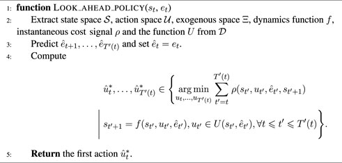
4.1 Look-ahead policy

The first of the policies introduced in our work, the look-ahead policy, is formally described in this section. We assume that this policy can predict exogenous variables up to a given time horizon K, denoted by policy horizon, ${\widehat{e}}_{t+1},\dots ,{\widehat{e}}_{T^{\prime }(t)}$ with 0⩽K ≪ T and T′(t) = min(t + K, T). With these predictions, the policy computes an open-loop sequence of actions ${\widehat{u}}_t^{*},\dots ,{\widehat{u}}_{T^{\prime }(t)}^{*}$ that minimises the sum of costs ${\sum }_{t^{\prime }=t}^{T^{\prime }(t)}\rho (s_{t^{\prime }},{\widehat{u}}_{t^{\prime }}^{*},{\widehat{e}}_{t^{\prime }},s_{t^{\prime }+1})$ at each discrete time step t and applies the first action of this sequence. Any suboptimality of the sequence of actions ${\widehat{u}}_t^{*},\dots ,{\widehat{u}}_{T^{\prime }(t)}^{*}$ will depend on the prediction error of the exogenous variable and the policy horizon K. Algorithm 1 presents this policy given a full definition of the decision process and a policy horizon. Furthermore, Algorithm 2 illustrates the interactions between the policy and the REC.

Algorithm 1. Look-ahead policy for decision process $\mathcal{D}$ and policy horizon K.

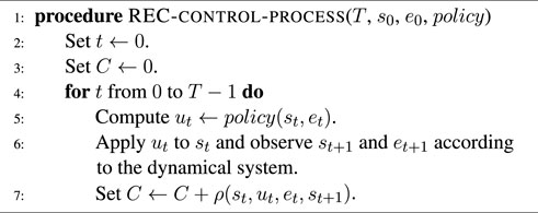
Algorithm 2. REC control process with a given policy.

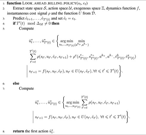
4.2 Look-ahead-billing policy

Improving upon the look-ahead policy, this section introduces the look-ahead-billing policy. When using the look-ahead policy, the billing costs related to the repartition keys for the last metering period of the optimisation time horizon are often not taken into account. Indeed, let $i\in {\mathbb{N}}^{+}$ be the lowest value such that (i + 1)Δ_M > T′(t). If T′(t) ≠ (i + 1)Δ_M, or in others words, if T′t) does not coincide with the end of the metering period ]iΔ_M, (i + 1)Δ_M], the term ρ^e corresponding to this metering period would not be included in the objective function (see Algorithm 1). In this situation, the actions ${\widehat{u}}_t^{*}$ may significantly differ from those which would be computed by optimising the cost of the electricity bill including T′(t). Taking into account a cost related to the repartition keys may improve the quality of the policy. To this end, we introduce virtual repartition keys, denoted by $a^{k_{-}}$ and $a^{k_{+}}$, which follow the same constraints as $u^{k_{-}}$ and $u_{k_{+}}$ as described in Section 3. They also follow the same constraints as the variables $u^{k_{-}}$ and $u_{k_{+}}$, which are defined at the metering period to which T′(t) belongs. However, we consider this latter condition to be implicit so as to keep the description of the policy below a reasonable level of complexity. These virtual repartition keys are introduced as decision variables in the optimisation problem solved by the look-ahead policy, whenever the last time step does not correspond to the end of a metering period. Moreover, an extra term ρ^e can be added to the objective function, depending on these new virtual repartition keys. With such a change, the objective function when T’(t) does not correspond to the end of a metering period writes:

$\begin{array}{ll}\hfill & \underset{\begin{array}{c}{u}_t,\dots ,u_{T^{\prime }\left(t\right)}\\ a^{k_{+}},a^{k_{-}}\end{array}}{\min }\left[\sum _{t^{\prime }=t}^{T^{\prime }\left(t\right)}\rho \left(s_{t^{\prime }},u_{t^{\prime }},{\widehat{e}}_{t^{\prime }},s_{t^{\prime }+1}\right)\right.\hfill \\ \hfill & +\left.{\rho }^e\left(s_{T^{\prime }\left(t\right)}^{e_{-}},s_{T^{\prime }\left(t\right)}^{e_{+}},a^{k_{+}},a^{k_{-}},{\widehat{e}}_{T^{\prime }\left(t\right)}^b,{\widehat{e}}_{T^{\prime }\left(t\right)}^s\right)\right].\hfill \end{array}(12)$

Algorithm 3 constructs this new policy with a full definition of the decision process and a policy horizon as inputs. Later in the simulation, we demonstrate show and discuss the performances of the two policies on different scenarios.

Algorithm 3. Look-ahead-billing policy for decision process $\mathcal{D}$ and policy horizon K.

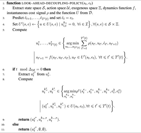
4.3 Look-ahead-decoupling policy

Depending on the complexity of the optimisation problem to be solved at each discrete time step–especially when K is rather large–the computation time needed for the look-ahead and look-ahead-billing policies might not be compatible with real-time constraints of the control actions. Indeed, these two policies jointly optimise both control actions and repartition keys, and this optimisation procedure creates greater complexity than optimising only the control actions. If computational constraints are an issue, the two optimisations can be decoupled so that the control actions are first optimised and then, based on them, an ex-post optimisation of the repartition keys can be performed, in a similar fashion than (Manuel de Villena et al., 2020b). This optimising procedure is computationally less intensive, but at the expense of the quality of the solution. Consequently, a trade-off between them emerges, which can only be assessed on a case-by-case analysis.

According to these principles, a new policy can be defined, namely the look-ahead-decoupling policy. This policy requires the export key $u_{+}^k$ to be restricted to zero during the computation of the sequence of actions. Then, given this sequence of actions, the sequence of repartition keys is optimised. This policy is inspired by (Manuel de Villena et al., 2020b) and adapted to our work. Algorithm 4 describes the look-ahead-decoupling policy. Note that, in practice, the computation of the repartition keys can be done outside the REC control process described in Algorithm 2 so as to further decrease the complexity of this policy.

Algorithm 4. Look-ahead-decoupling policy for decision process $\mathcal{D}$ and policy horizon K.

4.4 Computing open-loop sequences of actions for the three policies

To compute open-loop sequences of actions for each of the policies, we assume that, at each discrete time step t, all the policies have access to the exogenous variables e_t, …, e_T′(t) for all look-ahead horizons $K\in {\mathbb{N}}^{+}$ and for all time horizons $T\in {\mathbb{N}}^{+}$. Moreover, to encode this problem as a linear or mixed-integer linear program, we need to linearise the transition dynamics, constraints and cost functions. Then, the policies can exploit any available mixed-integer linear program solver such as CPLEX (Cplex, 2009) to compute open-loop sequences of actions in a time-receding horizon fashion during the control process of this REC. This section presents the linearisations needed to encode and solve the problem using such an off-the-shelf MILP solver.

4.4.1 Linearisation of the transition dynamics functions

Let us first define the indicator function 1₌₀(x), indicating whether x is zero:

${\mathbf{1}}_{=0}\left(x\right)=\left\{\begin{array}{cc}1\hfill & \mathbf{i}\mathbf{f}x=0,\hfill \\ 0\hfill & \mathbf{o}\mathbf{t}\mathbf{h}\mathbf{e}\mathbf{r}\mathbf{w}\mathbf{i}\mathbf{s}\mathbf{e}.\hfill \end{array}\right.(13)$

Since the value of s^τ is known, the transition functions $f^{e_{+}}$ and $f^{e_{+}}$ can be transformed into equivalent linear functions as follows.

$f^{e_{+}}\left(s_i^{e_{+}},l_i^{+}\right)={\mathbf{1}}_{=0}\left(s^{\tau }\right)s_i^{e_{+}}+l_i^{+},\forall i\in \mathcal{I},\forall s\in \mathcal{S},(14)$

$f^{e_{-}}\left(s_i^{e_{-}},l_i^{-}\right)={\mathbf{1}}_{=0}\left(s^{\tau }\right)s_i^{e_{-}}+l_i^{-},\forall i\in \mathcal{I},\forall s\in \mathcal{S}.(15)$

4.4.2 Linearisation of the constraints

Let us derive ${\mathcal{U}}^{\prime }$ from $\mathcal{U}$ by replacing import and export key $u^{k_{-}}$ and $u^{k_{+}}$ by electricity imported from retailer $u^{\prime r_{-}}$, electricity exported to retailer $u^{\prime r_{+}}$, electricity imported locally $u^{\prime l_{-}}$, and electricity exported locally $u^{\prime l_{+}}$. Let U′ be a set of admissible actions equivalent to U for all $(s,e)\in \mathcal{S}\times \mathrm{\Xi }$.

$U^{\prime }\left(s,e\right)\subseteq \left\{\begin{array}{cc}\hfill & \left\{\left[\left(u_1^c,\dots ,u_N^c\right),\varnothing ,\varnothing \right]\in {\mathcal{U}}^{\prime }\right\}\mathbf{i}\mathbf{f}{s}_t^{\tau }\ne 0,\hfill \\ \hfill & \left\{\left.\left[\left(u_1^c,\dots ,u_N^c\right),u^{\prime r_{+}},u^{\prime r_{-}},u^{\prime l_{+}},u^{\prime l_{-}}\right]\in {\mathcal{U}}^{\prime }\right|\right.\hfill \\ \hfill & \left(u_i^{\prime r_{+}},u_i^{\prime r_{-}},u_i^{\prime l_{+}},u_i^{\prime l_{-}}\right)\in {\mathbb{N}}^{+}\mathbf{a}\mathbf{n}\mathbf{d}\hfill \\ \hfill & u_i^{\prime r_{+}}+u_i^{\prime l_{+}}⩽s_i^{e_{+}}\mathbf{a}\mathbf{n}\mathbf{d}\hfill \\ \hfill & \sum _{i\in I}{u^{\prime l_{+}}}_i=\sum _{i\in I}{u^{\prime l_{-}}}_i\mathbf{a}\mathbf{n}\mathbf{d}\hfill \\ \hfill & \left.\left(u_i^{\prime r_{-}}+u_i^{\prime l_{-}}\right)-\left(u_i^{\prime r_{+}}+u_i^{\prime l_{+}}\right)=s_i^{e_{-}}-s_i^{e_{+}},\forall i\in \mathcal{I}\right\}\mathbf{o}\mathbf{t}\mathbf{h}\mathbf{e}\mathbf{r}\mathbf{w}\mathbf{i}\mathbf{s}\mathbf{e}.\hfill \end{array}\right..(16)$

We then can replace, for all $i\in \mathcal{I}$, the constraints on the repartition keys described by Eq. 2 with the following constraints.

$u_i^{r_{+}}=0,(17)$

$u_i^{r_{-}}=0,(18)$

4.4.3 Linearisation of the whole cost function

Since the value of f^τ(s^τ) is known, the cost function ρ can be transformed into an equivalent linear function as follows:

$\begin{array}{ll}\hfill \rho \left(s_t,u_t,e_t,s_{t+1}\right)& ={\mathbf{1}}_{=0}\left(f^{\tau }\left(s^{\tau }\right)\right){\rho }^e\left(s_t^{e_{-}},s_t^{e_{+}},u_t^{k_{-}},u_t^{k_{+}},e_t^b,e_t^s\right)\hfill \\ \hfill & +\sum _{i\in \mathcal{I}}{\rho }_i^o\left(s_{i,t}^c,u_{i,t}^c,e_{i,t}^o,s_{i,t+1}^c\right).\hfill \end{array}(19)$

5 Testing the policies on a REC decision process constructed from synthetic data

In this section, we illustrate and test the three policies proposed in Section 4. To that end, we employ various policy horizons and three different RECs (Cases 0, I and II). The former, detailed in Section 5.1, is a simple REC with two members, a producer equipped with a battery and a consumer, so as to illustrate the working principle of the three policies. The two others are constructed from synthetic data, and inspired from a real-life case of REC that was in operation from 2017 till 2021 in the municipality of Méry, Belgium (Cornélusse et al., 2017).

Case I The first REC includes six members: four consumers, one producer based on a solar photovoltaic (PV) installation, and the owner of a large lithium-ion battery. The latter is, therefore, the only controllable asset of the REC.

Case II The second case is similar to the first, but differs on specific points: i) the lithium-ion battery is replaced by a long-term storage device with larger capacity but less power capacity, and ii) the PV producer also owns a small lithium-ion battery, suitable for short-term storage. Hydrogen-based storage systems can be used as long-term storage whereby relatively large amounts of energy can be economically stored since the container is inexpensive. However, due to the high costs of electrolytes and cells, their power is usually limited. On the other hand, lithium-ion batteries are relatively expensive at high capacities, but they provide relatively inexpensive input and output power, which make them good candidates for short-term electricity storage. This second REC is inspired by the single user off-grid microgrid set-up described in (Francois et al., 2016).

Finally, we display and discuss the results, particularly highlighting the difference in terms of performances between jointly optimising the controllable assets and the repartition keys, and optimising only the controllable assets. We also report the runtime of the three policies tested in the two REC cases with a Dell XPS 15, equipped with a Intel Core i7 3.5 GHz CPU and 16 GB of DDR4 RAM. Note that the computational complexity of each policy correspond to the underlying linear solver we have used (Cplex, 2009) which itself has a complex behaviour depending on the number of variables and the general shape of the model.

Due to the scarcity of the available data and the fact that the computation of the policies are deterministic at runtime, we focus our experiments on a single consumption and production profiles for each REC member. However, as shown by results in Sections 5.2.4 and 5.3.3, the performance of the policies are sufficiently different to compare them, particularly between the look-ahead policy and the look-ahead-decoupling policy.

5.1 Description of case 0

In this section, we formalise a simple REC composed of N = 2 members. The first member, named C, is a consumer. The second member, named PVB, is a PV producer equipped with a battery.

5.1.1 Discretisation of the time horizon

We assume that the duration between two discrete time steps Δ_C is set to 1 h and that the number of time steps in a metering period Δ_M is 4. We assume that the time horizon T is 24 h.

5.1.2 State space

The member C has no controllable asset, so $s_1^c$ is empty. The member PVB has a battery and its state $s_2^c\in {\mathbb{R}}_{+}$ is its state of charge, expressed in kWh.

5.1.3 Action space

Since the member C has no controllable asset, the action $u_1^c$ is empty. The battery of the member PVB can be charged by the action $u_2^{c_{+}}\in {\mathbb{R}}_{+}$ and discharged by the action $u_2^{c_{-}}\in {\mathbb{R}}_{+}$. Both actions are expressed in kW. The action $u_2^c\in {\mathbb{R}}_{+}^2$ is defined as $(u_2^{c_{+}},u_2^{c_{-}})$.

5.1.4 Exogenous space

Figure 3 shows the consumption profile of member C and the production profile of member PVB. The values of the exogenous variables $e_{t,1}^o\in {\mathbb{R}}_{+}$ and $e_{t,2}^o\in {\mathbb{R}}_{+}$ correspond to these respective profiles.

FIGURE 3

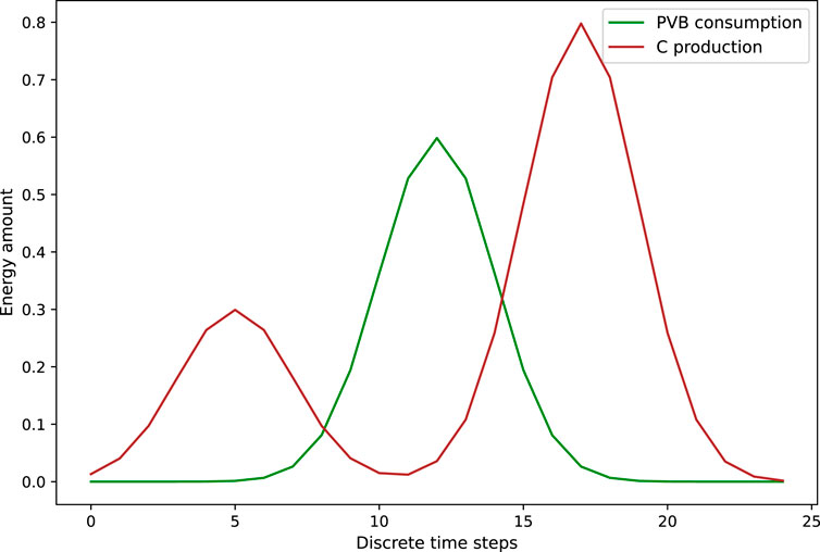
FIGURE 3. Consumption profile of the member C and production profile of the member PVB for the REC of Case 0.

The retailer contracts of the members C and PVB specify that they are charged at 1€/kWh and 2€/kWh for electricity consumption, respectively. These retailer contracts also specify that the surplus of electricity production of these members injected into the network is not bought back. In other words, the selling prices are 0.

The values of $e_i^b=\left[e_1^{rb}\right]$, $e_2^b=\left[e_2^{rb}\right]$, $e_1^s=\left[e_1^{rs}\right]$, $e_2^s=\left[e_2^{rs}\right]$ are set accordingly.

5.1.5 Constraints on the action space

The actions related to the battery of member PVB are bounded by the content and power capacities as follows.

$s_2^c-u_2^{c_{+}}⩾0,(20)$

$s_2^c+u_2^{c_{-}}⩽1,(21)$

$u_2^{c_{+}}⩽0.05,(22)$

$u_2^{c_{-}}⩽0.01.(23)$

5.1.6 Net electricity consumption/production during a control period

The net electricity production and consumption of the member C are based on its consumption profile. More formally, the values of $l_1^{+}$ and $l_1^{-}$ are set to 0 and $e_1^o$, respectively. The net electricity production and consumption of the member PVB are based on its production profile and the activity of its battery. More formally, the values of $l_2^{+}$ and $l_2^{-}$ are set to $e_2^o+u_2^{c_{+}}$ and $u_2^{c_{-}}$, respectively.

5.1.7 Transition dynamics

Since the member C has no controllable asset, no transition dynamics is associated to him. The transition function associated to the member PVB, which continuously charge and discharge its battery, is defined as follows:

$f_2^c\left(s_2^c,u_2^c,e_2^o\right)=s_2^c+u_2^{c_{+}}-u_2^{c_{-}}.(24)$

The initial state $S_2^c$ is set to 0.33.

5.1.8 Cost functions

Since the member C has no controllable asset, the operational cost ${\rho }_1^o$ of the member C is fixed to 0. The operational cost ${\rho }_2^o$ of the member PVB is defined as ${\rho }_2^o(s_2^c,u_2^c,e_2^o,s_2^{\prime c})=10^{-6}{u}_2^{c_{-}}$ so as to introduce mutual exclusion between charge and discharge commands (see Section 5.2.1 for a detailed explanation).

The total combined value of the individual electricity bills depending on the repartition keys ρ^e is defined as:

$\begin{array}{ll}\hfill {\rho }^e\left(s^{e_{-}},s^{e_{+}},u^{k_{-}},u^{k_{+}},e^b,e^s\right)& =\sum _{i=1}^2\left(s_i^{e_{-}}-u_i^{k_{-}}\mathrm{\Phi }\right)e_i^{rb}\hfill \\ \hfill & -\left(1-u_i^{k_{+}}{s}_i^{e_{+}}\right)e_i^{rs}.\hfill \end{array}(25)$

See Section 5.2.3 for the linearisation of this cost function.

5.1.8.1 Illustrating the policies through case 0

Table 1 shows the results of testing the three policies with $K\in \left\{\mathrm{4,8,12}\right\}$ and the optimal policy (equivalent to K = T = 24). Note that the total combined value of the individual electricity bills only corresponds to the electricity bill of the member C. Figure 4 shows the evolution of the state of charge of the battery by testing the three policies with $K\in \left\{\mathrm{4,8}\right\}$ and the optimal policy.

TABLE 1

TABLE 1. Size (in financial terms) of the electricity bill of member C by testing the three policies with several policy horizons for the simple REC, compared with the optimal policy (equivalent to the look-ahead policy with K = T = 24). The electricity bill of PVB is not shown in this table; its value is 0 for all policies tested.

FIGURE 4

FIGURE 4. State of the battery and total electricity consumption covered by surplus of electricity production (local electricity net consumption) at each discrete time step for Case 0.

The optimal policy handles at best the intermittence of the solar production of the member PVB by charging at most during the production peak and discharging at the consumption peak that occurs later in the day. In the other hand the look-ahead-decoupling policy, which has the worst performance, does not use at all the battery. In this case, the look-ahead-billing policy is consistently, slightly better than the look-ahead policy. At K = 4, the look-ahead policy completely discharges the battery to satisfy the first consumption peak and do not use the battery afterwards, while the look-ahead-billing policy uses a little fraction of the production peak to charge the battery before discharging at the end of the day. As K grows, the behaviour of the two policies gets closer to the optimal policy.

5.2 Description of case I

5.2.1 Formal description of the decision process

This section completes the formulation of the decision process associated with the first REC, composed of N = 6 members, where i) 1, …, 4 are the indexes referring to four consumers named C1, …, C4, ii) the 5th member is a PV producer named PV, and iii) the 6th member is a battery owner named B who does not consume or produce electricity via non-controllable assets.

5.2.1.1 Discretisation of the time horizon

We assume that Δ_C = 0.25 h and that Δ_M = 4. We assume that T = 720, which corresponds to 7.5 days.

5.2.1.2 State space

The state $s_i^c$ for members $i\in \left\{1,\dots ,5\right\}$ is represented by an empty state s^∅. The state $s_6^c\in {\mathbb{R}}_{+}$ is the state of charge of battery of the member 6, expressed in kWh.

5.2.1.3 Action space

The action $u_i^c$ for members $i\in \left\{1,\dots ,5\right\}$ is represented by an empty action u^∅. The action $u_6^c\in {\mathbb{R}}_{+}^2$, defined as $(u_6^{c_{+}},u_6^{c_{-}})$, is a pair of charge/discharge commands of the battery owned by member 6, both expressed in kW.

5.2.1.4 Exogenous space

The exogenous variable $e_{t,i}^o\in {\mathbb{R}}_{+}$ is the amount of energy consumed by the non-controllable assets of member i at time step t expressed in kWh, for all members $i\in \left\{\mathrm{1,2,3,4}\right\}$ and for all time steps t = 0, …, T − 1. The exogenous variable $e_{t,5}^o$, for all time steps t = 0, …, T − 1, corresponds to the amount of energy produced by the photovoltaic installation of member five at time step t. Member six is not equipped with any non-controllable asset. Therefore, we set its exogenous variable $e_{t,6}^o$ to 0 for all time steps t = 0, …, T − 1. The consumption profiles of members 1, …, four and the production profile of member five are constructed from real-life consumption data⁴. The exogenous variables related to the price vectors of buying electricity for all members $i\in \mathcal{I}$ are defined as $e_i^b=\left[e_i^{rb}\right]$ where $e_i^{rb}\in {\mathbb{R}}_{+}$ is the retailer’s buying price for member i expressed in €/kWh. The exogenous variables related to the price vectors of selling electricity for all members $i\in \mathcal{I}$ are defined as $e_i^s=\left[e_i^{rs}\right]$ where $e_i^{rs}\in {\mathbb{R}}_{+}$ is the retailer’s selling price for the member i expressed in €/kWh. Purchasing retail prices for all members $i\in \mathcal{I}$ and the selling retail prices for members 5 and 6 are detailed in Section 5.2.2 for all discrete time steps t = 0, …, T − 1.

5.2.1.5 Constraints on the action space

The set of admissible actions U(s, e) for all pairs of states and exogenous variables $(s,e)\in \mathcal{S}\times \mathcal{E}$ is described by the following set of inequations.

$s_6^c-{\mathrm{\Delta }}_C\left({\eta }_6^{+}{u}_6^{c_{+}}\right.⩾S_6^{\lfloor c\rfloor },(26)$

$s_6^c+\frac{{\mathrm{\Delta }}_C{u}_6^{c_{-}}}{{\eta }_6^{-}}⩽S_6^{\lceil c\rceil },(27)$

$u_6^{c_{+}}⩽U_6^{\lceil c_{+}\rceil },(28)$

$u_6^{c_{-}}⩽U_6^{\lceil c_{-}\rceil },(29)$

where ${\eta }_6^{+}$ is the charging efficiency of the battery of member 6 and ${\eta }_6^{-}$ is the discharging efficiency of the battery of member 6, $S_6^{\lfloor c\rfloor }$ and $S_6^{\lceil c\rceil }$ are lower and upper bounds of the state of charge of the battery of member 6 expressed in kWh, respectively, and $U_6^{\lceil c_{+}\rceil }$ and $U_6^{\lceil c_{-}\rceil }$ are both upper bounds of the charge and discharge commands of the battery of member 6 expressed in kW, respectively. Eqs 26, 27 specify the upper and lower limits of the state of charge of the battery of member 6, respectively. Eqs 28, 29 specify the upper limits of the charge and discharge commands of the battery of member 6, respectively.

5.2.1.6 Net electricity consumption/production during a control period

The values of $l_i^{+}$ and $l_i^{-}$ for all members $i\in \mathcal{I}$ are defined by Table 2.

TABLE 2

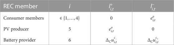
TABLE 2. Net electricity production and consumption of REC members for Case I.

5.2.1.7 Transition dynamics

Transition dynamics for all members except member 6, are defined as follows:

$f_i^c\left(s_i^c,u_i^c,e_i^o\right)=s_i^c,\forall i\in \left\{1,\dots ,5\right\}.$

Transition dynamics specific to the charging/discharging dynamics of the battery of the member 6 are defined as follows:

$f_6^c\left(s_6^c,u_6^c,e_6^o\right)=s_6^c+{\mathrm{\Delta }}_C\left({\eta }_6^{+}{u}_6^{c_{+}}-\frac{u_6^{c_{-}}}{{\eta }_6^{-}}\right).(30)$

5.2.1.8 Cost functions

We define the operational cost functions of all members $i\in \left\{1,\dots ,5\right\}$ as ${\rho }_6^o(s_i^c,u_i^c,e_i^o,s_i^{\prime c})=0$. We define the operational cost function for member 6 as ${\rho }_6^o(s_6^c,u_6^c,e_6^o,s_6^{\prime c})=ϵu_6^{c_{-}}$, where ϵ = 10^–6. This cost function is a small penalty on the discharge command of the battery so as to introduce a mutual exclusion between charge and discharge commands. Without such a penalty, applying null commands to the battery (i.e., $u_6^{c_{+}}=0$ and $u_6^{c_{-}}=0$) would be equivalent with respect to the optimisation objective defined in Eq. 10 to apply charging/discharging commands that cancel each other (i.e. ${\eta }_6^{+}{u}_6^{c_{+}}-\frac{u_6^{c_{-}}}{{\eta }_6^{-}}=0$), according to Eq. 30.

The total combined value of the individual electricity bills depending on the repartition keys ρ^e is defined as:

$\begin{array}{ll}\hfill {\rho }^e\left(s^{e_{-}},s^{e_{+}},u^{k_{-}},u^{k_{+}},e^b,e^s\right)& =\sum _{i\in \mathcal{I}}\left(s_i^{e_{-}}-u_i^{k_{-}}\mathrm{\Phi }\right)e_i^{rb}\hfill \\ \hfill & -\left(1-u_i^{k_{+}}{s}_i^{e_{+}}\right)e_i^{rs}.\hfill \end{array}(31)$

5.2.2 Values from synthetic data for case I

The sequences of exogenous variables related to the energy buying prices from retailers $e_i^{rb}$ and to the energy selling prices to retailers $e_i^{rs}$ for all members $i\in \mathcal{I}$, expressed in €/kWh, are also constructed from synthetic pricing plans as shown in Table 3.

TABLE 3

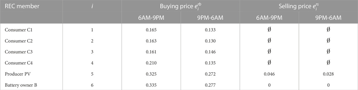
TABLE 3. Synthetic pricing plans for Cases I & II.

The values for parameters described in Section 5.2.1 and initial states are:

$\begin{array}{ll}\hfill S_{\mathrm{6,0}}^c& =300kWh,\hfill \\ \hfill {\eta }_6^{+}& ={\eta }_6^{-}=88\%,\hfill \\ \hfill S_6^{\lfloor c\rfloor }& =40kWh,\hfill \\ \hfill S_6^{\lceil c\rceil }& =160kWh,\hfill \\ \hfill U_6^{\lceil c_{+}\rceil }& =176kW,\hfill \\ \hfill U_6^{\lceil c_{-}\rceil }& =352kW.\hfill \end{array}$

5.2.3 Computing open-loop sequences of actions for each policy

The total combined value of the individual electricity bills defined by Eq. 31 can be transformed into an equivalent linear function using action space ${\mathcal{U}}^{\prime }$ as follows.

${\rho }^e\left(s^{e_{-}},s^{e_{+}},u^{\prime r_{-}},u^{\prime r_{+}},u^{\prime l_{-}},u^{\prime l_{+}},e^b,e^s\right)=\sum _{i\in \mathcal{I}}{u}_i^{\prime r_{-}}{e}_i^{rb}-u_i^{\prime r_{+}}{e}_i^{rs}.(32)$

5.2.4 Testing the policies for case I and discussion on results

The three policies discussed in Section 4 are tested in this section for Case I with varying policy horizons $K\in \left\{\mathrm{12,24,36,48}\right\}$. More specifically, we compare the results of the look-ahead and look-ahead-billing policies, which jointly optimise controllable assets and repartition keys over the policy horizon K, against the optimal policy–the equivalent to look-ahead with K = 720 and perfect information concerning all exogenous variables–and the look-ahead-decoupling policy which only optimises the controllable assets over the policy horizon K. Table 4 shows the results of this test. Table 5 shows the runtime of the policies during the tests, which essentially grows with K, the difference between the policies being very slight.

TABLE 4

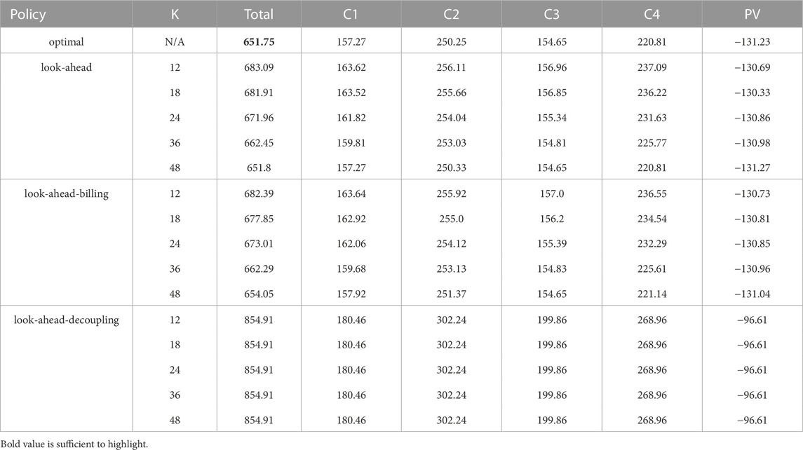
TABLE 4. Size (in financial terms) of the electricity bill in total and also for each member by testing the three policies with several policy horizons for the first REC, compared with the optimal policy (equivalent to the look-ahead policy with K = T = 720). Since the size of the electricity bill of the member 6 is 0 regardless of the tested policy, the corresponding column is not reported.

TABLE 5

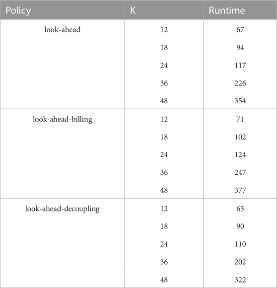
TABLE 5. Runtime (in seconds) of the three policies tested in the first REC.

The combined total value of the electricity bills of the members obtained by using the look-ahead policy with the policy horizon K = 12 is close to the one obtained using the optimal policy—the difference being less than 30€, and this difference decreases as K grows. At K = 48, the difference with the optimal policy is less than 0.05€. These results suggest that near-optimal open-loop sequences of actions can be computed with the look-ahead policy with a rather small policy horizon, provided that the prediction error on the exogenous variables is low.

The combined total value of the electricity bills of the members obtained by using the look-ahead-billing policy with the policy horizon K = 12 is lower than the look-ahead policy (by around 1€). This suggests that the look-ahead-billing policy, which computes virtual repartition keys at the last time step T′(t) might output better quality actions than the look-ahead policy. When K grows, we make the same observations as in the results of Case I.

Regardless of the policy horizon K, the combined total value of the electricity bills of the members obtained by using the look-ahead-decoupling policy is significantly higher than the one obtained using the optimal policy (by around 200€). Since this amount is also significantly higher compared to the other policies within the same REC configuration, it clearly shows the importance, for any efficient open-loop policy, of computing sequences of actions by jointly optimising the controllable assets and the repartition keys through the control process of a REC.

To better understand the difference in terms of the combined total value of the electricity bills of the members across the policies, Figure 5 shows the evolution of the state of charge of the battery of member 6. We notice that, while the optimal policy and the look-ahead policy make use of the battery of member 6 the look-ahead-decoupling policy does not use it at all. This is expected since the look-ahead-decoupling policy cannot compute the repartition keys in real time, and therefore cannot use the demand and production of the community to charge and discharge the battery.

FIGURE 5

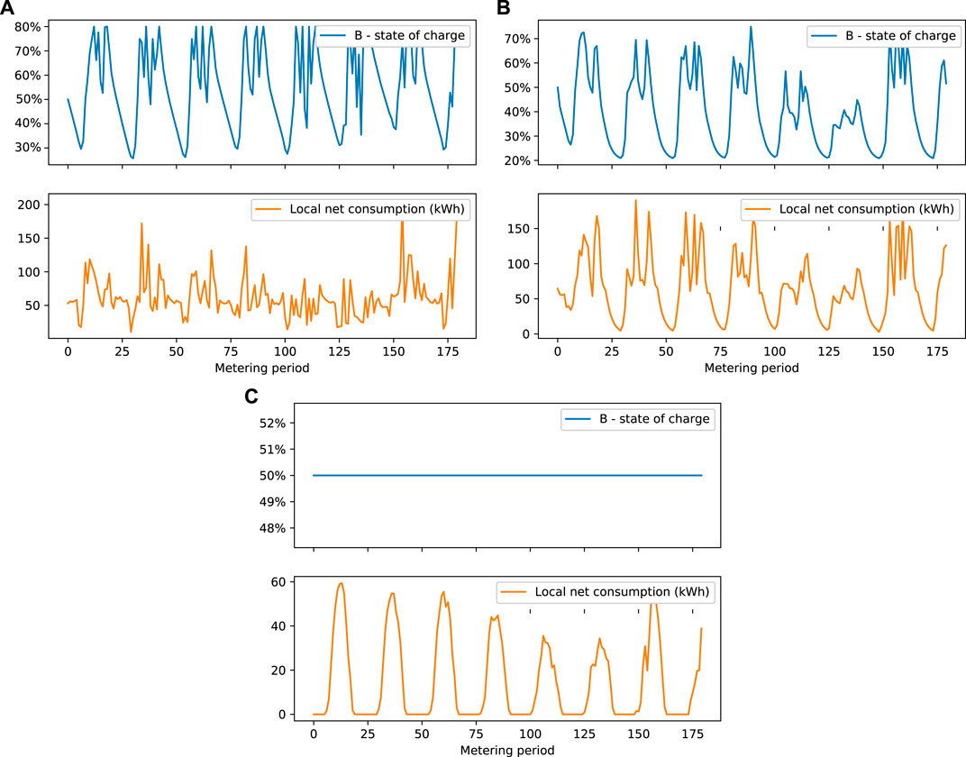
FIGURE 5. State of the battery and total electricity consumption covered by surplus of electricity production (local electricity net consumption) at each discrete time step for Case I.

Results also show the individual electricity bills. Note that repartition keys implicitly define a rule to redistribute the global electricity bill among the members. At the end of each metering period, the look-ahead policy, look-ahead-billing policy and the optimal policy redistribute the local production surplus generated by members 5 and 6 to the other members. The way they redistribute it depends on their consumption profiles and their retailer tariffs. Indeed, according to Eq. 31, the import key allocated to members with higher retailer tariffs should be higher than the others, following a global minimisation criterion of the combined total value of the electricity bills.

5.3 Description of case II

5.3.1 Differences with the decision process of case I

This section describes the decision process associated with the second REC (case II), which only differs from the first one in that member 5 of the REC (i.e., the solar-based electricity producer) owns a small battery, and that the configuration of the battery of member 6 differs in terms of capacity, power and energy efficiency. More precisely, we describe the components of the decision process associated with this second REC which differs from the first one.

Spaces State $s_5^c$ and action $u_5^c$ share the same definitions as $s_6^c$ and $u_6^c$, respectively.

Constraints Upper and lower bounds on $s_5^c$ and action $u_5^c$ share the same definition as $s_6^c$ and $u_6^c$.

Production The variable $l_5^{+}$ is equal to $e_i^o+{\mathrm{\Delta }}_C{u}_i^{c_{-}}$.

Consumption The variable $l_5^{-}$ shares the same definition as $l_6^{-}$.

Dynamics The transition dynamics function $f_5^c$ shares the same definition as $f_6^c$.

Cost functions The cost function ${\rho }_5^o$ shares the same definition as ${\rho }_6^o$.

5.3.2 Values from synthetic data for case II

The values for parameters described in Sections 5.2.1 and 5.3.1 as well as initial states are set as follows.

$S_{\mathrm{5,0}}^c=37kWh,(33)$

${\eta }_5^{+}=99\%,(34)$

${\eta }_5^{-}=99\%,(35)$

$S_5^{\lfloor c\rfloor }=15kWh,(36)$

$S_5^{\lceil c\rceil }=60kWh,(37)$

$U_5^{\lceil c_{+}\rceil }=37kW,(38)$

$U_5^{\lceil c_{-}\rceil }=97kW,(39)$

$S_{\mathrm{6,0}}^c=250kWh,(40)$

${\eta }_6^{+}=83\%,(41)$

${\eta }_6^{-}=83\%,(42)$

$S_6^{\lfloor c\rfloor }=100kWh,(43)$

$S_6^{\lceil c\rceil }=400kWh,(44)$

$U_6^{\lceil c_{+}\rceil }=441kW,(45)$

$U_6^{\lceil c_{-}\rceil }=882kW.(46)$

5.3.3 Testing the policies for case II and discussion on results

As in Section 5.2.4, we test the three policies discussed in Section 4 in the second REC (case II) with varying policy horizons $K\in \left\{\mathrm{12,24,36,48}\right\}$. Table 6 shows the results of these tests. Table 7 shows the runtime of the policies during the tests, with the same observations as the first REC. However, the runtime of the policies are higher than for the first REC, which is expected since the number of variables is higher.

TABLE 6

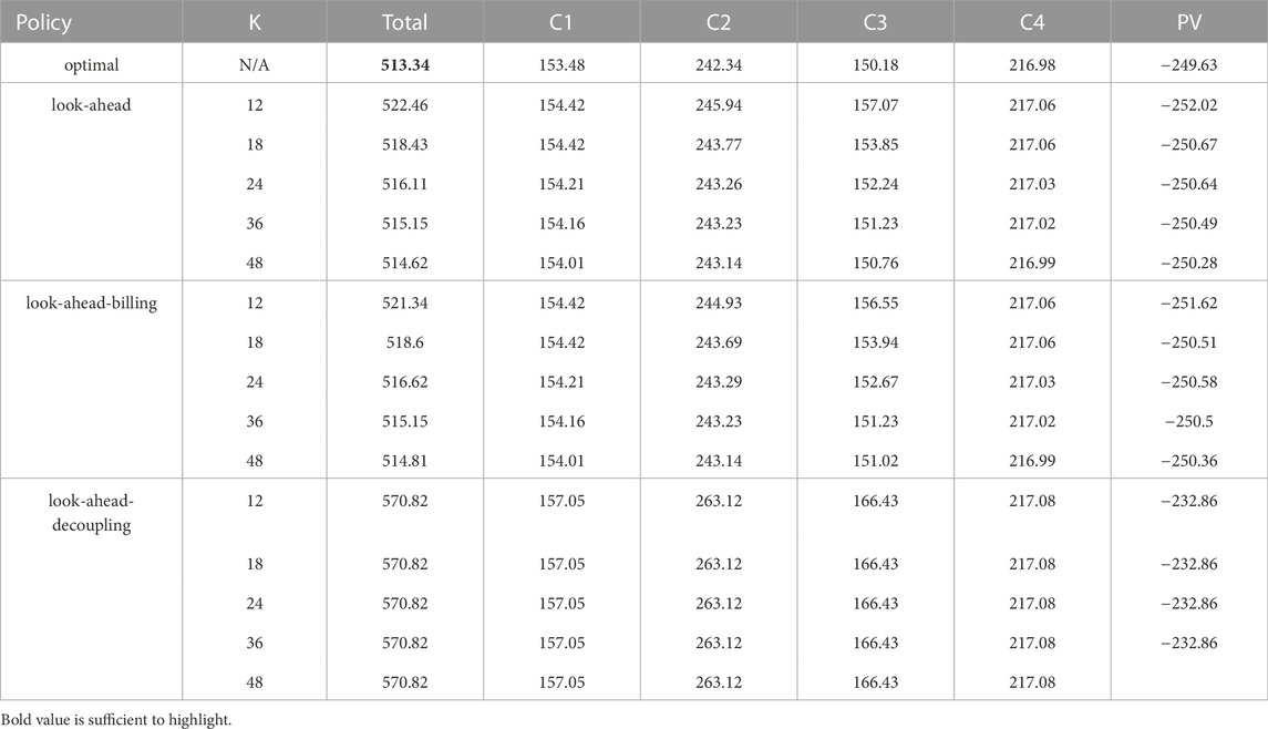
TABLE 6. Size (financial) of the overall electricity bill and those for each individual member by testing the three policies with several policy horizons for Case II, compared with the optimal policy (equivalent to the look-ahead policy with K = T = 720). Since the size of the electricity bill of the member 6 is 0 regardless of the tested policy, the corresponding column is not reported.

TABLE 7

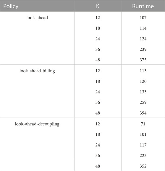
TABLE 7. Runtime (in seconds) of the three policies tested in the second REC.

The combined total value of the electricity bills of the members, obtained by using the look-ahead policy with the policy horizon K = 12 is similar to the one obtained using the optimal policy—the difference is less than 10€, and this difference decreases as K grows. At K = 48, the difference with the optimal policy is less than 1€. This corroborates that the near-optimal open-loop sequences of actions can be computed with the look-ahead policy with a rather small policy horizon, provided that there is a low prediction error of the exogenous variables.

The combined total value of the electricity bills of the members, obtained by using the look-ahead-billing policy with the policy horizon K = 12 is lower than the look-ahead policy (around 1€). As in the previous policy, as K grows, the difference between their sub-optimalities decreases. Indeed, the combined total value of the electricity bills of the members obtained by using the look-ahead billing policy with the policy horizon K = 48 is lower than that obtained through the look-ahead policy. It is also interesting to note that across the values of K, the combined total value of the electricity bills obtained by the look-ahead billing policy is lower than the one obtained by the look-ahead policy, which validates the hypothesis that the look-ahead billing policy can improve the quality of the control actions compared to the look-ahead policy.

Regardless of the policy horizon K, the combined total value of the electricity bills of the members obtained by using the look-ahead-decoupling policy is significantly higher than the one obtained using the optimal policy (by around than 50€).

To better understand the difference in terms of the combined total value of the electricity bills of the members across the policies, Figure 6 shows the evolution of the state of charge of the battery of member 6. As in the first REC, we notice that the look-ahead-decoupling policy does not use the battery at all, unlike the two other policies. However, the battery owned by member 5 is also used by this policy, and it is used in a different way to the two other policies. The pattern of the state of charge of the battery suggests that this battery discharges its energy to sell it to its own retailer when the selling price is higher than outside this time interval.

FIGURE 6

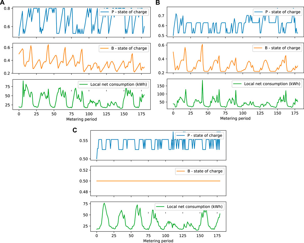
FIGURE 6. State of the batteries and total electricity consumption covered by surplus of electricity production (local electricity net consumption) at each discrete time step for Case II.

6 Conclusion and perspectives

In this paper, we have proposed a generic formulation of the decision process associated with renewable energy communities, which enables one to jointly optimise the controllable assets of each member and the repartition keys used to allocate the local production among the members in order to minimise the total combined value of their individual electricity bills. We have proposed two policies that exploit both the structure of the REC and the available predictions of the future production and consumption of each member to perform this joint optimisation in a time-receding horizon fashion. Furthermore, a third policy that only optimises the controllable assets is proposed. We have tested these algorithms on two REC control problems constructed from synthetic data with 6 members–4 consumers, one producer and a battery. Our results highlight the importance of the joint optimisation of the controllable assets and the repartition keys, as higher total combined value of individual electricity bills have been observed for the third policy.

The contribution of this paper could be extended along several directions. First, let us observe that the control policies we have proposed have been using linear programming techniques since the dynamics and the cost functions associated with the REC constructed from synthetic data were linear - this is often not the case for real RECs. In such context, we could use more advanced techniques such as non-linear programming techniques (e.g., interior point methods) in these open-loop policies or even use closed-loop policies. Reinforcement learning techniques (Bellman, 1954), especially by exploiting the expressiveness of deep neural networks (François-Lavet et al., 2018) (Mnih et al., 2015) (Lillicrap et al., 2015), are excellent candidates to construct these closed-loop policies, since these techniques have been successfully tested on challenging control problems related to microgrids and power systems (Tomin et al., 2019; François-Lavet et al., 2016; Glavic et al., 2017). Another interesting avenue for future research would also be to conduct a extensive benchmark on the look-ahead and the look-ahead-billing policies to extract an insight on which situations one of the policies is more efficient than the other one.

Finally, the repartition keys, introduced by the decision process developed in Section 3, implicitly describe a mechanism to redistribute the revenues generated from the REC, which corresponds to the difference between the combined total value of the individual electricity bills without the REC and the combined total value of the individual electricity bills with the REC. However, this redistribution of the REC revenues is biased by the electricity tariffs imposed by the retailers on each member. Indeed, as observed by the simulation results in Section 5, whenever the buying retail tariff of a member is higher compared to other members, the size of its individual electricity bill is lower compared to these members. By design, other factors that could influence this redistribution in another way (e.g., investment participation of a member to build the REC, subsides brought by some members) are not taken into account at optimisation stage. An ex-post procedure could be developed to compute alternative redistributions schemes as to better incentivise the members to join the RECs.

Data availability statement

Publicly available datasets were analyzed in this study. This data can be found here: https://zenodo.org/record/6047543#.Yg_VBdvjLd5 (only first column of each file).

Author contributions

SA and DE designed the research. QG has helped with the research and the design of the software architecture to conduct the experiments. SA performed the research. SA and MdV collected the data. SA, MdV, and GD drafted the manuscript. MdV, MC, GD, QG, and DE provided feedback on the research and manuscript. All authors contributed to the article and approved the submitted version.

Funding

The authors gratefully acknowledge the support of the Walloon region through the funding of the Merygrid and Integcer projects.

Conflict of interest

QG was employed by Haulogy.

The remaining authors declare that the research was conducted in the absence of any commercial or financial relationships that could be construed as a potential conflict of interest.

Publisher’s note

All claims expressed in this article are solely those of the authors and do not necessarily represent those of their affiliated organizations, or those of the publisher, the editors and the reviewers. Any product that may be evaluated in this article, or claim that may be made by its manufacturer, is not guaranteed or endorsed by the publisher.

Footnotes

¹According to the latest European regulation, any end customer–consumer or prosumer–may participate in a REC without losing the previous status.

²$\mathcal{P}$ is the notation for the power set.

³The objective function might be a different one (e.g., expected value at risk).

⁴Consumption and production profiles are publicly available on Zenodo, see (Aittahar et al., 2022). Consider only the column 1st week of each file.

References

Aittahar, S., de Villena, M. M., Derval, G., Castronovo, M., Boukas, I., Gemine, Q., et al. (2022). Optimal control of renewable energy communities with controllable assets: Consumption and production profiles. doi:10.5281/zenodo.6047543

CrossRef Full Text | Google Scholar

Bellman, R. (1954). The theory of dynamic programming. Tech. rep. Washington: Rand corp santa monica ca.

Google Scholar

Boukas, I., Ernst, D., and Cornélusse, B. (2018). CIRED 2018 ljubljana workshop on microgrids and local energy communities.Real-time bidding strategies from micro-grids using reinforcement learning.

Google Scholar

Ciocia, A., Di Leo, P., Malgaroli, G., and Spertino, F. (2020). “Subhour simulation of a microgrid of all-electric nzebs based on Italian market rules,” in 2020 IEEE international conference on environment and electrical engineering and 2020 IEEE industrial and commercial power systems europe (EEEIC/ICPS europe), 1–6. doi:10.1109/EEEIC/ICPSEurope49358.2020.9160517

CrossRef Full Text | Google Scholar

Code de l’énergie Français (2017). Article D315-6, créé par Décret 2017-676 du 28 avril 2017 - art, 2.

Google Scholar

Cominesi, S. R., Farina, M., Giulioni, L., Picasso, B., and Scattolini, R. (2017). A two-layer stochastic model predictive control scheme for microgrids. IEEE Trans. Control Syst. Technol. 26, 1–13.

Google Scholar

Cornélusse, B., Ernst, D., Warichet, L., and Legros, W. (2017). Efficient management of a connected microgrid in Belgium. CIRED-Open Access Proc. J. 2017, 1729–1732. doi:10.1049/oap-cired.2017.0211

CrossRef Full Text | Google Scholar

Cornélusse, B., Savelli, I., Paoletti, S., Giannitrapani, A., and Vicino, A. (2019). A community microgrid architecture with an internal local market. Appl. Energy 242, 547–560. doi:10.1016/j.apenergy.2019.03.109

CrossRef Full Text | Google Scholar

Cplex, I. I. (2009). V12. 1: User’s manual for cplex. Int. Bus. Mach. Corp. 46, 157.

Google Scholar

Ernst, D., Glavic, M., Capitanescu, F., and Wehenkel, L. (2009). Reinforcement learning versus model predictive control: A comparison on a power system problem. IEEE Trans. Syst. Man, Cybern. Part B Cybern. 39, 517–529. doi:10.1109/TSMCB.2008.2007630

PubMed Abstract | CrossRef Full Text | Google Scholar

European Union(2018). Directive 2018/2001 of the European Parliament and of the Council of 11 december 2018 on the promotion of the use of energy from renewable sources. Official J. Eur. Union 4, 82–209.

Google Scholar

Francois, V., Gemine, Q., Ernst, D., and Fonteneau, R. (2016). Towards the minimization of the levelized energy costs of microgrids using both long-term and short-term storage devices, 295–319. doi:10.1201/b19664-17

CrossRef Full Text | Google Scholar

François-Lavet, V., Henderson, P., Islam, R., Bellemare, M. G., and Pineau, J. (2018). An introduction to deep reinforcement learning. CoRR abs/1811.12560.

Google Scholar

François-Lavet, V., Taralla, D., Ernst, D., and Fonteneau, R. (2016). “Deep reinforcement learning solutions for energy microgrids management,” in European workshop on reinforcement learning, Barcelona (EWRL).

Google Scholar

Glavic, M., Fonteneau, R., and Ernst, D. (2017). Reinforcement learning for electric power system decision and control: Past considerations and perspectives. IFAC-PapersOnLine 50, 6918–6927. doi:10.1016/j.ifacol.2017.08.1217

CrossRef Full Text | Google Scholar

Heaslip (nee Hassett), E., Costello, G., and Lohan, J. (2016). Assessing good-practice frameworks for the development of sustainable energy communities in Europe: Lessons from Denmark and Ireland. J. Sustain. Dev. Energy, Water Environ. Syst. 4, 307–319. doi:10.13044/j.sdewes.2016.04.0024

CrossRef Full Text | Google Scholar

Hooshmand, A., Poursaeidi, M. H., Mohammadpour, J., Malki, H. A., and Grigoriads, K. (2012). “Stochastic model predictive control method for microgrid management,” in 2012 IEEE PES innovative smart grid technologies (ISGT), 1–7. doi:10.1109/ISGT.2012.6175660

CrossRef Full Text | Google Scholar

Lillicrap, T. P., Hunt, J. J., Pritzel, A., Heess, N., Erez, T., Tassa, Y., et al. (2015). Continuous control with deep reinforcement learning. arXiv preprint arXiv:1509.02971.

Google Scholar

Manuel de Villena, M., Boukas, I., Mathieu, S., Vermeulen, E., and Ernst, D. (2020a). “A framework to integrate flexibility bids into energy communities to improve self-consumption,” in 2020 IEEE general meeting (IEEE), 1–5.

CrossRef Full Text | Google Scholar

Manuel de Villena, M., Gautier, A., Ernst, D., Glavic, M., and Fonteneau, R. (2021). Modelling and assessing the impact of the DSO remuneration strategy on its interaction with electricity users. Int. J. Electr. Power & Energy Syst. 126, 106585. doi:10.1016/j.ijepes.2020.106585

CrossRef Full Text | Google Scholar

Manuel de Villena, M., Mathieu, S., Vermeulen, E., and Ernst, D. (2020b). Allocation of locally generated electricity in renewable energy communities. arXiv preprint arXiv:2009.05411.

Google Scholar

Mathieu, S., Manuel de Villena, M., Vermeulen, E., and Ernst, D. (2019). “Harnessing the flexibility of energy management systems: A retailer perspective,” in 2019 IEEE milan PowerTech (IEEE), 1–6.

CrossRef Full Text | Google Scholar

Mnih, V., Kavukcuoglu, K., Silver, D., Rusu, A. A., Veness, J., Bellemare, M. G., et al. (2015). Human-level control through deep reinforcement learning. Nature 518, 529–533. doi:10.1038/nature14236

PubMed Abstract | CrossRef Full Text | Google Scholar

Moret, F., and Pinson, P. (2018). Energy collectives: A community and fairness based approach to future electricity markets. IEEE Trans. Power Syst. 34, 3994–4004. doi:10.1109/tpwrs.2018.2808961

CrossRef Full Text | Google Scholar

Nakabi, T. A., and Toivanen, P. (2020). Deep reinforcement learning for energy management in a microgrid with flexible demand. Sustain. Energy, Grids Netw. 25, 100413. doi:10.1016/j.segan.2020.100413

CrossRef Full Text | Google Scholar

Oreshkin, B. N., Dudek, G., Pełka, P., and Turkina, E. (2021). N-beats neural network for mid-term electricity load forecasting. Appl. Energy 293, 116918. doi:10.1016/j.apenergy.2021.116918

CrossRef Full Text | Google Scholar

Parisio, A., and Glielmo, L. (2011). “Energy efficient microgrid management using model predictive control,” in 2011 50th IEEE conference on decision and control and European control conference (IEEE), 5449–5454.

CrossRef Full Text | Google Scholar

Prasad, A., and Dusparic, I. (2019). IEEE PES innovative smart grid technologies europe (ISGT-Europe). 1–5. doi:10.1109/ISGTEurope.2019.8905628Multi-agent deep reinforcement learning for zero energy communities

CrossRef Full Text | Google Scholar

Reijnders, V. M., van der Laan, M. D., and Dijkstra, R. (2020). “Chapter 6 - energy communities: A Dutch case study,” in Behind and beyond the meter. Editor F. Sioshansi (Academic Press), 137–155. doi:10.1016/B978-0-12-819951-0.00006-2

CrossRef Full Text | Google Scholar

Service public de Wallonie (2019). Mai 2019 – Décret modifiant les décrets des 12 avril 2001 relatif à l’organisation du marché régional de l’électricité, du 19 décembre 2002.

Google Scholar

Sousa, T., Soares, T., Pinson, P., Moret, F., Baroche, T., and Sorin, E. (2019). Peer-to-peer and community-based markets: A comprehensive review. Renew. Sustain. Energy Rev. 104, 367–378. doi:10.1016/j.rser.2019.01.036

CrossRef Full Text | Google Scholar

Sutton, R. S., and Barto, A. G. (2018). Reinforcement learning: An introduction. MIT press.

Google Scholar

Tomin, N., Zhukov, A., and Domyshev, A. (2019). Deep reinforcement learning for energy microgrids management considering flexible energy sources. EPJ Web Conf. 217, 01016. doi:10.1051/epjconf/201921701016

CrossRef Full Text | Google Scholar

Torabi Moghadam, S., Di Nicoli, M. V., Manzo, S., and Lombardi, P. (2020). Mainstreaming energy communities in the transition to a low-carbon future: A methodological approach. Energies 13, 1597. doi:10.3390/en13071597

CrossRef Full Text | Google Scholar

Tushar, W., Yuen, C., Mohsenian-Rad, H., Saha, T., Poor, H. V., and Wood, K. L. (2018). Transforming energy networks via peer-to-peer energy trading: The potential of game-theoretic approaches. IEEE Signal Process. Mag. 35, 90–111. doi:10.1109/msp.2018.2818327

CrossRef Full Text | Google Scholar

Zhou, S., Hu, Z., Gu, W., Jiang, M., and Zhang, X. (2019). Artificial intelligence based smart energy community management: A reinforcement learning approach. CSEE J. Power Energy Syst. 5, 1–10. doi:10.17775/CSEEJPES.2018.00840

CrossRef Full Text | Google Scholar