Quarterly GDP forecast based on coupled economic and energy feature WA-LSTM model

Existing macroeconomic forecasting methods primarily focus on the characteristics of economic data, but they overlook the energy-related features concealed behind these economic characteristics, which may lead to inaccurate GDP predictions. Therefore, this paper meticulously analyzes the relationship between energy big data and economic data indicators, explores the coupling feature mining of energy big data and economic data, and constructs features coupling economic and energy data. Targeting the nonlinear variation coupling features in China’s quarterly GDP data and using the long short-term memory (LSTM) neural network model based on deep learning, we employ wavelet analysis technology (WA) to decompose selected macroeconomic variables and construct a prediction model combining LSTM and WA, which is further compared with multiple benchmark models. The research findings show that, in terms of quarterly GDP data prediction, the combined deep learning model and wavelet analysis significantly outperform other methods. When processing structurally complex, nonlinear, and multi-variable data, the LSTM and WA combined prediction model demonstrate better generalization capabilities, with its prediction accuracy generally surpassing other benchmark models.

1 Introduction

With the development of economic globalization, we are faced with new opportunities and challenges, and the fluctuations in the global economy are having an increasingly significant impact on China’s domestic economy. Therefore, conducting accurate economic forecasts, formulating appropriate economic policies, and avoiding economic risks in advance have become particularly important. Quarterly GDP metrics offer benefits in showcasing crucial macroeconomic figures like the quarterly economic total and growth rate, and they can promptly illustrate recent trends in economic development, thus having significant reference value in formulating economic policies. Exploring high-precision statistical methods for predicting quarterly GDP and revealing the laws of GDP changes on a quarterly basis is of great importance in macroeconomic development planning.

In reality, GDP growth isn’t solely influenced by the cyclical fluctuations of the macroeconomy. Other energy variables, including energy production and consumption, can also play a role in shaping the short, medium, and long-term trajectories of GDP. Hence, when assessing GDP trends, it’s essential to consider both macroeconomic factors and an array of other specific determinants (Huang et al., 2021; Huang et al., 2022).

To substantiate this, numerous researchers have delved deeper. For instance, Das et al. (2012) employed a system matrix estimation technique to analyze the electricity consumption and GDP data of 45 developing countries over the last 4 decades, revealing a positive correlation between the two. Similarly, ZAshraf, AYJavid, and MJavid from Pakistan (Ashraf et al., 2013) reached a parallel conclusion. Furthermore, Altinay Galip and Karagol Erdal (Altinay and Karagol, 2005) affirmed this through a causality perspective. However, research from the U.S. Energy Information Administration suggests the relationship might vary across countries. Research by KraftJ, Stern D1 (Kraft and Kraft, 1978), Ferguson R (Ferguson et al., 2000) and Liu (Liu et al., 2023) further underscored the tight bond between energy consumption and economic growth.

Over the years, researchers have primarily relied on traditional linear prediction models for GDP forecasting. For instance, The linear time series forecasting model, known as the autoregressive integrated moving average (ARIMA), a concept brought forward by Box and Jenkins in 1976 (Box and Jenkins, 2010), stands as a notable example in this field. Considering the seasonality of economic data, researchers further discussed the applicability of seasonal ARIMA models in cyclical economic time series (Ngungu et al., 2018). However, many studies have overlooked other influencing factors when predicting GDP and only used univariate models, which are prone to data leakage, resulting in biased prediction accuracy. In contrast, the vector autoregression (VAR) model incorporates more prediction variables, and Linda F. Debenedictis (Debenedictis, 1997) found that the VAR model outperforms the ARIMA model in predicting actual GDP values. In the selection of other variables, Linda F. Debenedictis introduced traditional economic indicators such as the money supply (M2) and fixed assets investment (INVESTMENT) as prediction variables.

Currently, an increasing number of scholars are applying machine learning techniques to data prediction (Tan et al., 2022). Artificial Neural Networks (ANN), as a prominent example of machine learning algorithms, can handle complex nonlinear multidimensional data. Tkacz (2001) (Tkacz, 2001) applied the ANN model to the research on the annual GDP growth rate prediction in Canada, showing that the model prediction error was reduced by about 25% compared to linear prediction models. With the advancement of computer performance, deep learning has gradually become the frontier field of machine learning and has received extensive attention in economic data prediction. X. Wu, Z (Wu et al., 2021) believes that deep neural network models such as neural network models such as Long Short-Term Memory (LSTM) and Convolutional Neural Network (CNN) are superior to traditional ARIMA, VAR, and other models in predicting economic data. Furthermore, some scholars found that utilizing wavelet analysis (WA) to decompose time series can better extract features, thereby improving model prediction accuracy. Yan et al. (2019) applied wavelet analysis to the prediction of individual household energy consumption, and the empirical results showed that the integration of wavelet analysis improved the predictive performance of dynamic trends in time series. However, few studies have applied wavelet analysis techniques to GDP data prediction.

In this study, we employed the LSTM model combined with wavelet analysis to decompose nine critical macroeconomic variables. To enhance prediction accuracy, we identified four energy indicators with strong relevance to GDP. During the model’s development, we utilized time series cross-validation to refine the parameters, leading to the creation of an integrated LSTM and wavelet analysis prediction model (LSTM&WA), primarily applied to forecast China’s quarterly GDP data. To assess the performance of our model, we compared it with various forecasting models, including SARIMA, VAR, ANN, 1D-CNN, and their wavelet-augmented counterparts like VAR&WA, ANN&WA, and 1D-CNN&WA. Additionally, we examined the prediction accuracy changes before and after incorporating energy indicators. This comprehensive analysis enabled us to evaluate the efficacy and reliability of different models in predicting China’s GDP data.

The main contributions and organization are given as follows:

• The article provides a detailed analysis of the relationship between energy big data and economic indicators, carries out mining of the coupling characteristics between energy big data and economic data, and constructs the coupling characteristics of economic data and energy data.

• Considering the nonlinear change characteristics of China’s quarterly GDP, the LSTM model from deep learning neural networks is introduced, combined with wavelet analysis technology to decompose the selected macroeconomic variables. Subsequently, an LSTM & WA (Wavelet Analysis) forecasting model is constructed to conduct predictive research on the high and low frequency parts of the quarterly GDP.

• Comparative analysis of the predictive effects of various models (LSTM, 1D-CNN & WA, 1D-CNN, ANN & WA, ANN, VAR & WA, VAR) shows that the LSTM & WA forecasting model has better generalization capability, and its prediction accuracy surpasses the other seven benchmark models.

The following text outlines the organization of this paper. Section two presents an LSTM neural network model for economic forecasting. Section three conducts a case study, offering prediction outcomes and associated errors. Finally, Section four provides a summary of the primary contributions of this paper.

2 Model building

In order to verify whether deep learning models are applicable for economic data prediction, this paper selects commonly used models in economic data prediction, such as SARIMA, VAR, and the ANN model from shallow machine learning as the benchmark models, aiming to compare the GDP prediction capabilities of different models. The specific construction of SARIMA, VAR, and ANN models can be found in references (Debenedictis, 1997; Tkacz, 2001; Ngungu et al., 2018; Tan et al., 2022).

2.1 Deep learning models

2.1.1 CNN model

CNN is a type of feedforward neural network that can be used in areas such as image and speech recognition. Unlike multilayer feedforward neural networks, CNN has fewer network structure parameters and features local connections, weight sharing, and subsampling. A typical CNN network structure is composed of interconnected convolutional and pooling layers, supplemented by fully connected layers. Initially, the raw data is fed into the CNN network where it experiences several simultaneous convolutional processes, generating a variety of feature maps. These maps are subsequently modified via a nonlinear activation function, like ReLU. Next, pooling layers compress the generated features by choosing either the maximum value, known as max pooling, or the mean value, termed average pooling within a specific region from the results generated by the convolutional layer, with the aim of decreasing the quantities of parameters and lessening the computational burden in the subsequent layer., and prevent overfitting. The final layer is a fully connected one, essentially embodying a conventional neural network architecture, whose essence is to combine features generated from the previous convolutional layers and set different parameters.

Figure 1 shows the overall architecture of the CNN network, Figure 2 depicts feature map transformations, Figure 3 illustrates receptive field changes, and Figure 4 presents the basic structure of the one-dimensional CNN network used in this study, mainly including two one-dimensional convolutional layers and two average pooling layers, etc.

FIGURE 1

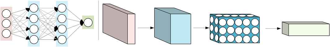
FIGURE 1. Overall architecture of CNN network.

FIGURE 2

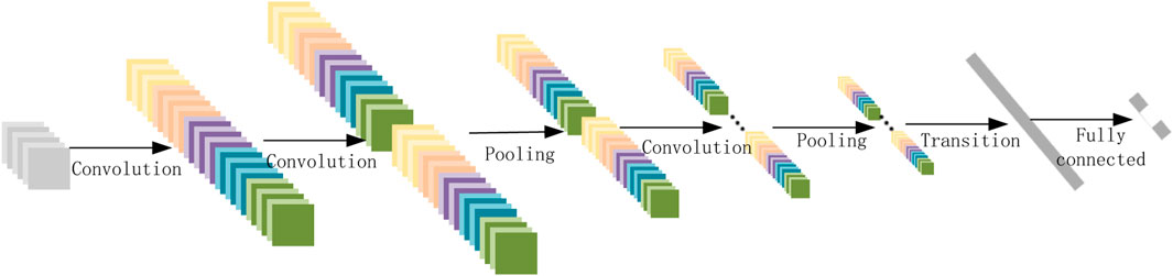
FIGURE 2. Feature map transformation.

FIGURE 3

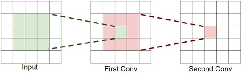
FIGURE 3. Change in receptive field.

FIGURE 4

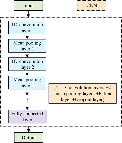
FIGURE 4. 1D-CNN model structure.

2.1.2 LSTM model

When using Long Short-Term Memory networks (LSTM) for quarterly GDP forecasting based on the coupling of economic and energy data, LSTMs have several advantages over Convolutional Neural Networks (CNN), so we adopt LSTM model to forecast GDP.

• Sequence Learning Ability: LSTM is designed to handle sequence data, capable of capturing long-term dependencies within time series, which is very useful for predicting economic indicators like GDP.

• Handling Variable-Length Sequences: LSTM can process time series data of varying lengths, while CNN typically requires fixed-size inputs.

• Forgetting Mechanism: LSTM has a forgetting gate that enables them to learn to ignore irrelevant information, which is an important feature when analyzing complex economic and energy data.

• Stable Learning Process: LSTM is generally more stable than CNN when processing long time sequences and have a relatively smaller problem with vanishing gradients.

As the LSTM neural network model can better discover long-distance dependence relationships in sequence data, it is widely used in handling time series data issues. At the same time, the LSTM model is proficient at addressing the issues of gradient explosion and gradient disappearance during the learning process. The basic principle of LSTM is to record and use the state of all previous positions to better represent the short-distance and long-distance dependencies in the sequence data. LSTM’s cell structure introduces two mechanisms, namely, “memory cells” and “gates.” The former records the state information of previous positions, while the latter controls the state information usage through gate functions. These three gates’ functions are to protect and control the cell state, determining whether the information will be passed on to the next cell.

The LSTM network mainly consists of LSTM layers and Dropout layers, and the LSTM model structure can be seen in Figure 5.

FIGURE 5

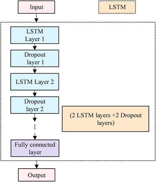
FIGURE 5. LSTM model structure.

2.1.3 Model structure

The 1D-CNN network’s input layer takes charge of accepting the one-dimensional time series input data X = [x₁, x₂, x_n] to undergo network processing. The convolutional layer extracts input features by applying dot product operations on the input vector, weights, and biases, and an activation function is applied for nonlinear mapping while the pooling layer condenses the outcomes produced by the convolutional layer, performing average pooling on selected regions. Convolution and pooling operations are as follows:

${\mathrm{C}}_1=\mathrm{f}\left(\mathrm{X}\otimes {\mathrm{w}}_1+{\mathrm{b}}_1\right)=\text{ReLU}\left(\mathrm{X}\otimes {\mathrm{w}}_1+{\mathrm{b}}_1\right)(1)$

${\mathrm{p}}_1=\text{average}\left({\mathrm{C}}_1\right)+{\mathrm{b}}_2(2)$

${\mathrm{C}}_2=\mathrm{f}\left(\mathrm{X}\otimes {\mathrm{w}}_2+{\mathrm{b}}_3\right)=\text{ReLU}\left({\mathrm{p}}_1\otimes {\mathrm{w}}_2+{\mathrm{b}}_3\right)(3)$

${\mathrm{p}}_2=\text{average}\left({\mathrm{C}}_2\right)+{\mathrm{b}}_4(4)$

${\mathrm{H}}_2=\mathrm{f}\left({\mathrm{p}}_2\otimes {\mathrm{w}}_3+{\mathrm{b}}_5\right)=\text{sigmoid}\left({\mathrm{p}}_2\otimes {\mathrm{w}}_3+{\mathrm{b}}_5\right)(5)$

Where C₁ and C₂ are the output vectors of convolutional layers 1 and 2, respectively; p₁ and p₂ are the outputs of pooling layers 1 and 2, respectively; Weight matrices are denoted as w₁, w₂, and w₃, while b₁, b₂, b₃, b₄, and b₅ represent bias vectors. The outcome post convolutional and pooling operations is referred to as ${\mathrm{H}}_{\mathrm{c}}=\left[{\mathrm{h}}_{\mathrm{c}1},{\mathrm{h}}_{\mathrm{c}2},\cdots {\mathrm{h}}_{\text{ci}}\right]$, where i is the length of the output sequence; average represents average pooling; ReLU and Sigmoid are activation functions; And $\otimes$ is the dot product operation symbol.

Between the pooling layer and the fully connected layer, a Flatten layer is utilized to simplify the feature map into a one-dimensional vector, and a Dropout layer is employed to prevent overfitting, further improving the model’s generalization capability. The fully connected layer uses activation functions to allocate weights on feature vectors, and iteratively updates the optimal weight parameter matrix for interpreting features extracted by the model’s convolutional part. The activation function learns load change rules from the extracted features to achieve the prediction function, and obtains the prediction results in the output layer. In this study, the activation function of the output layer is Linear, and the output layer calculation formula is:

${\mathrm{y}}_{\mathrm{t}}={\mathrm{w}}_0{\mathrm{a}}_{\mathrm{t}}+{\mathrm{b}}_0(6)$

Where ${\mathrm{y}}_{\mathrm{t}}$ is the output result of the tth network training, w₀ and b₀ are the weight matrix and bias vector, respectively.

For the LSTM model, an LSTM cell structure is shown in Figure 6. The LSTM neural network contains multiple cell structures.

${\mathrm{i}}_{\mathrm{t}}=\mathrm{\sigma }\left({\mathrm{x}}_{\mathrm{t}}{\mathrm{W}}_{\text{xi}}+{\mathrm{h}}_{\mathrm{t}-1}{\mathrm{W}}_{\text{hi}}+{\mathrm{b}}_{\mathrm{i}}\right)(7)$

${\mathrm{f}}_{\mathrm{t}}=\mathrm{\sigma }\left({\mathrm{x}}_{\mathrm{t}}{\mathrm{W}}_{\text{xf}}+{\mathrm{h}}_{\mathrm{t}-1}{\mathrm{W}}_{\text{hf}}+{\mathrm{b}}_{\mathrm{f}}\right)(8)$

${\stackrel{\sim }{\mathrm{c}}}_{\mathrm{t}}=\tanh \left({\mathrm{x}}_{\mathrm{t}}{\mathrm{W}}_{\text{xc}}+{\mathrm{h}}_{\mathrm{t}-1}{\mathrm{W}}_{\text{hc}}+{\mathrm{b}}_{\mathrm{c}}\right)(9)$

${\mathrm{c}}_{\mathrm{t}}={\mathrm{f}}_{\mathrm{t}}\otimes {\mathrm{c}}_{\mathrm{t}-1}+{\mathrm{i}}_{\mathrm{t}}\otimes {\stackrel{\sim }{\mathrm{c}}}_{\mathrm{t}}(10)$

${\mathrm{o}}_{\mathrm{t}}=\mathrm{\sigma }\left({\mathrm{x}}_{\mathrm{t}}{\mathrm{W}}_{\text{xo}}+{\mathrm{h}}_{\mathrm{t}-1}{\mathrm{W}}_{\text{ho}}+{\mathrm{b}}_{\mathrm{o}}\right)(11)$

${\mathrm{h}}_{\mathrm{t}}={\mathrm{o}}_{\mathrm{t}}\otimes \text{Linear}\left({\mathrm{c}}_{\mathrm{t}}\right)(12)$

FIGURE 6

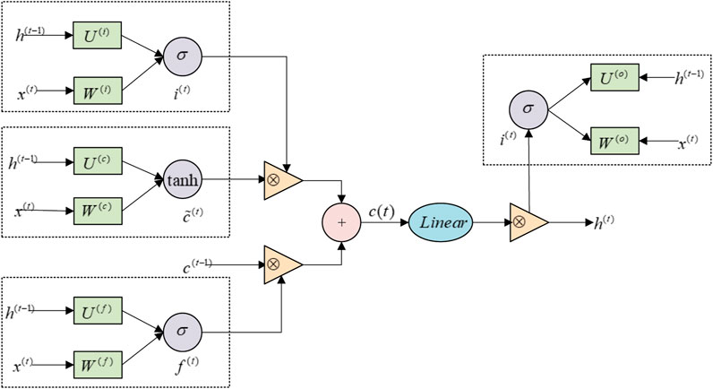
FIGURE 6. LSTM unit structure.

In this model, x_t is the input vector at time t, which includes historical data of macroeconomic variables such as quarterly GDP, M2, and CPI; ht-1 represents the output at the previous moment; c_t-1 denotes the memory at the previous moment; it indicates the output of the input gate; ft represents the output of the forget gate; refers to the memory updated at this moment; c_t stands for the final memory of the memory module; o_t describes the information filtered by the output gate that is not useful for prediction; h_t signifies the ultimate output of the output gate; W₁ and W₂ are weight matrices, and b₁ and b₂ are bias vectors; Tanh and Linear are activation functions.

2.2 Cross-validation to determine optimal parameters

In this study, cross-validation is employed to identify the parameters or hyperparameters for the selected models. The original dataset is divided into three categories: a training set, a validation set, and a test set. By iterating through parameter combinations in the training set and selecting the best parameter combination with the validation set using the rolling window cross-validation method. As shown in Figure 7, the validation set (Valid) is divided into 5-fold, each fold containing n samples. Compute RMSE1 with Train1 as the first training set and Valid1 as the first test set. Add n1 periods of samples to the training set, use Train2 as the second training set, Valid2 as the second test set, and calculate RMSE2. So on and so forth, the training set adds n samples each time and ends when Valid5 becomes the test set, then calculates RMSE5. Finally, the average RMSE is calculated based on the training results of the 5 validation sets to select better performing model parameters. Cross-validation improves the robustness of the model, does not produce significant outlier predictions, and makes the results more stable and reliable.

FIGURE 7

FIGURE 7. 5-fold cross-validation with rolling window.

SARIMA, VAR, ANN, and 1D-CNN models were selected as comparison models for LSTM in this paper. Due to the seasonal factors of the GDP sequence increasing with the overall trend, a multiplicative form of the SARIMA model was chosen. The optimal lag order for the VAR model is determined through the Akaike Information Criterion (AIC) and a VAR (1) model is established. In addition, a two-hidden-layer ANN model was considered.

The paper used a rolling window cross-validation method to tune and train SARIMA, VAR, ANN, 1D-CNN, and LSTM models on the data from the first quarter of 1996 to the second quarter of 2019 (74 quarters for training and 20 quarters for validation) and finally tested the GDP for 5 quarters. Throughout the training phase of neural network models, optimizers are required to enhance the model, refresh network model parameters, and establish varying parameters for adaptive learning rates., thereby improving training speed and prediction accuracy. Kingma and Ba (2014) compared several optimization algorithms, and the results showed that the Adam algorithm is a combination of ideas from gradient descent, momentum, and other stochastic optimization algorithms with slight improvements, and is an excellent algorithm in both computational power and performance. Therefore, the Adam algorithm was chosen as the optimizer for the selected neural network models in this paper.

Through the time series cross-validation tuning method mentioned above, the final parameter setups for the models developed in this research are showcased in the Table 1.

TABLE 1

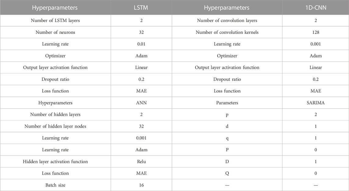
TABLE 1. Hyperparameters of the model.

To form a unified measurement standard among different prediction models, this study employs Root Mean Square Error (RMSE), Mean Absolute Error (MAE), and Mean Absolute Percentage Error (MAPE) as assessment metrics. The calculation formulas are as follows:

$\text{RMSE}=\sqrt{\frac{1}{\mathrm{N}}{\displaystyle \sum _{\mathrm{t}=1}^{\mathrm{N}}}{\left({\mathrm{y}}_{\mathrm{t}}-{\widehat{\mathrm{y}}}_{\mathrm{t}}\right)}^2}(13)$

$\text{MAE}=\frac{1}{\mathrm{N}}{\displaystyle \sum _{\mathrm{t}=1}^{\mathrm{N}}}\left|{\mathrm{y}}_{\mathrm{t}}-{\widehat{\mathrm{y}}}_{\mathrm{t}}\right|(14)$

$\text{MAPE}=\frac{100\%}{\mathrm{N}}{\displaystyle \sum _{\mathrm{t}=1}^{\mathrm{N}}}\left|\frac{{\mathrm{y}}_{\mathrm{t}}-{\widehat{\mathrm{y}}}_{\mathrm{t}}}{{\mathrm{y}}_{\mathrm{t}}}\right|(15)$

2.3 Wavelet analysis

Wavelet analysis adjusts the frequency spectrum and spatial positioning of data via the scaling and translation of the wavelet basis function. It identifies the oscillation frequency of data in time and spatial dimensions, consequently facilitating feature selection and noise reduction. Wavelet analysis technique disassembles input time series data into components of low and high frequencies. As the scale increases, the amplitude of wavelet coefficients in the high-frequency part diminishes to zero, portraying the transient random fluctuations in the sequence. The amplitude of the low-frequency part remains roughly the same, with no significant changes, capturing the fundamental pattern exhibited by the sequence.

By processing the features with wavelet analysis, the LSTM neural network model becomes less susceptible to the disruptive influence of short-term noise disturbances.

When forecasting quarterly GDP based on the coupling of economic and energy data, the first step is to process the economic features. The advantages of applying wavelet analysis over Fast Fourier Transform (FFT) include:

✓ Wavelet analysis is better suited for non-stationary data where the statistical properties change over time, which is often the case with economic data.

✓ Wavelet transforms provide both time and frequency information, allowing for a more detailed analysis of time series that have transient characteristics in specific time periods.

✓ They can handle abrupt changes and localized features in economic and energy data more effectively than FFT, which assumes the signal is periodic and continuous.

✓ Wavelets allow for multi-resolution analysis, which can be particularly useful for capturing the inherent hierarchies and multiple scales present in economic data.

3 Case study

3.1 Feature analysis

3.1.1 Economic data feature analysis

Based on Keynes’ theory, the following specific indicators are selected:

(1) Quarterly real GDP (GDP), which is the core variable for prediction;

(2) Money supply (M2), which represents changes in the money supply;

(3) Fixed asset investment completion amount (INVESTMENT), which as an important part of investment, is a crucial basis for monitoring macroeconomic trends;

(4) CPI month-on-month growth rate (CPI), which measures inflation levels;

(5) RMB loan benchmark interest rate (RATE), which is the short-term loan interest rate for lending periods within 6 months (inclusive of 6 months);

(6) Total retail sales of consumer goods (C), which reflects domestic consumption and can determine macroeconomic development trends;

(7) Export amount (EXPORT), which measures market openness, and when the indicator is large, it implies increased exports and good economic performance, otherwise, it indicates macroeconomic downturn;

(8) National public fiscal expenditure (Public Expenditure), representing the government’s purchasing situation;

(9) Month-to-month expansion rate of industrial value-added for enterprises above a designated size (Industrial Value), which is commonly used to judge the short-term industrial economic operation and macroeconomic prosperity.

The above data are from the website of the National Bureau of Statistics and the Wind database. Among these, 4 indicators are quarterly, and 5 are monthly. Considering that the core variable GDP is quarterly data, as shown in Figure 8, the frequencies of the 9 selected indicators need to be unified and all processed as quarterly data. The frequency statistics and particular processing techniques for each indicator are depicted in the fourth and fifth columns of Figure 8. The selected indicators cover a time span from the first quarter of 1996 (1996Q1) to the third quarter of 2020 (2020Q3). The explanations and descriptive statistics for each indicator are presented in Tables 2, 3.

FIGURE 8

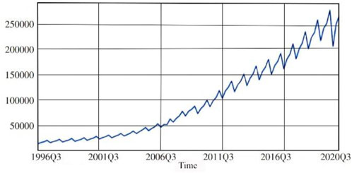
FIGURE 8. China’s quarterly GDP sequence from 1996 to 2020.

TABLE 2

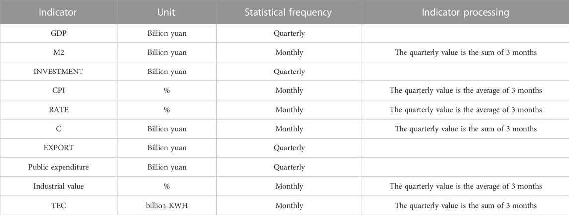
TABLE 2. Definitions and processing methods of the indicators.

TABLE 3

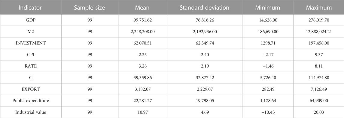
TABLE 3. Descriptive statistics of the indicators.

3.1.2 Energy data feature analysis

In terms of energy indicators, this paper also selects 10 related influencing factors in the energy economy, including power and energy, elements that notably influence economic production. The impact of these 10 factors on GDP is determined through grey relational analysis, and the specific grey correlation degree results are shown in Table 4.

TABLE 4

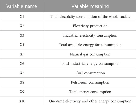
TABLE 4. Energy indicator names and meanings.

Through Table 5, it can be found that among the 10 indicators selected in this paper, X10 has the highest grey correlation degree with GDP, while X7 has the lowest. According to the ranking from high to low, this paper selects the top four variables as the main indicators affecting GDP, namely, X10, X9, X2, and X1, which are total social electricity consumption, electricity production, total energy consumption, and the consumption of primary electricity and other energy sources.

TABLE 5

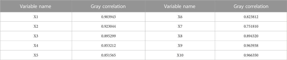
TABLE 5. Grey correlation degree.

3.2 Data preprocessing

3.2.1 Data normalization

In order to enhance the model’s training process and expedite its convergence speed, measures will be taken to optimize its performance, this paper uses the min-max standardization method for data normalization, as shown in Formula 16. After modeling and predicting using the normalized data, Formula 17 is used to restore the data for accuracy comparison among different models.

${\mathrm{x}}_{\text{scaled}}=\frac{\mathrm{x}-{\mathrm{x}}_{\min }}{{\mathrm{x}}_{\max }-{\mathrm{x}}_{\min }}(16)$

${\mathrm{x}}_{\text{unscale}}={\mathrm{x}}_{\text{scaled}}\left({\mathrm{x}}_{\max }-{\mathrm{x}}_{\min }\right)+{\mathrm{x}}_{\min }(17)$

This paper uses the multivariate time series from 1996Q1 to 2019Q2 as input values to establish ANN, 1D-CNN, and LSTM models. Due to the processing of lagged data by two periods, in order to ensure that the length of the input data for the model is the same, the total amount of data used is reduced from 94 sets to 92 sets.

3.2.2 Wavelet analysis

The four-stage compactly supported orthogonal wavelet (Daubechies wavelet, db4) has advantages such as better regularity, asymmetry, and strong time-frequency localization ability, which can increase the frequency domain resolution. Therefore, this paper selects db4 wavelet to perform wavelet analysis on selected macroeconomic variables and quarterly GDP, and draws waveform diagrams before and after analysis. This paper primarily examines the decomposition findings of the month-on-month growth rate of CPI, total retail sales of consumer goods, and national public fiscal expenditure, and China’s quarterly real GDP, as shown in Figures 9–12 on the next page.

FIGURE 9

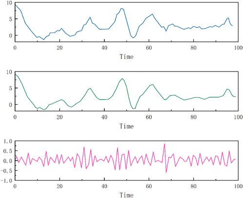
FIGURE 9. Wavelet decomposition results for CPI month-on-month growth rate.

FIGURE 10

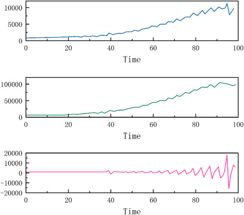
FIGURE 10. Wavelet decomposition results for total retail sales of consumer goods.

FIGURE 11

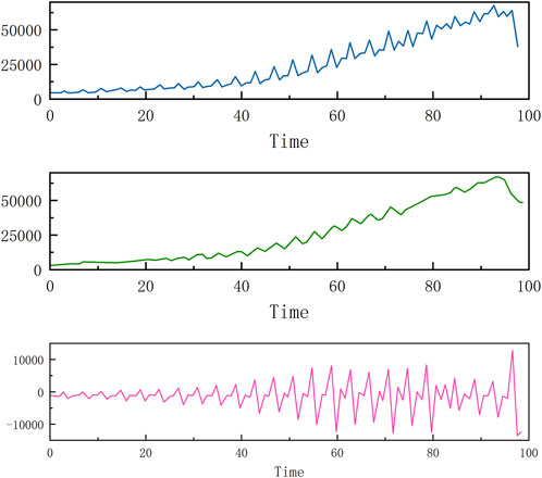
FIGURE 11. Wavelet decomposition results for national public fiscal expenditure.

FIGURE 12

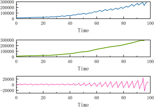
FIGURE 12. Wavelet decomposition results for China’s quarterly GDP.

It can be seen that each indicator presents different fluctuations on the original overall trend, and after wavelet analysis processing, the changes in the low-frequency part (the second subplot in each figure) are relatively smooth, reflecting an overall trend, while the high-frequency part (the third subplot in each figure) has a higher fluctuation frequency and more frequent changes.

Next, this paper builds VAR&WA, ANN&WA, 1D-CNN&WA, and LSTM&WA models for the high and low-frequency parts, respectively, and finally compares the combined predictions with the actual GDP values.

3.3 Model prediction ability comparison analysis

This paper uses a rolling forecast method for prediction, that is, using known true values for predicting the next period. Figure 13 illustrates the prediction process using a 3-step rolling forecast as an example. To obtain prior sample information, quarterly GDP data from lag 1 to lag 4 is used as the initial sample interval. From the 5th period onwards, a one-step forward rolling forecast is performed, that is, estimating the 5th period’s quarterly GDP data based on prior information, obtaining the predicted value Fore_5 for the 5th period. The true value of GDP, True_5, for the 5th period is added to the initial sample to predict the 6th period’s quarterly GDP data, and so on, until predicting the 7th period’s quarterly GDP.

FIGURE 13

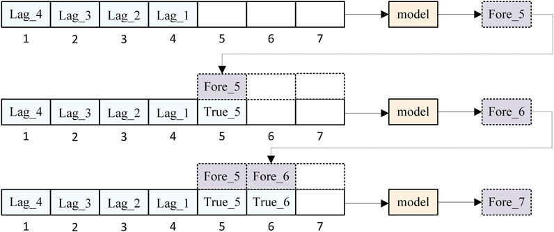
FIGURE 13. Rolling forecast method for predicting 3 periods.

3.3.1 Univariate model prediction performance

This paper establishes SARIMA (2,1,1) × (0,1,0)4, VAR (1), ANN, 1D-CNN, and LSTM models and, after verification, conducts rolling forecasts on China’s quarterly GDP (a total of 5 data points) from 2019Q3 to 2020Q3. Since the SARIMA model can only predict a single time series, for ease of analysis, we model the univariate quarterly GDP data. The prediction results of various models are presented in Table 6, illustrating the univariate analysis, and the last two columns of Table 6 provide the RMSE and MAPE of these four models for the GDP time series. As can be seen, deep learning neural network models’ prediction performance is superior to other machine learning models, such as the ANN model, and traditional seasonal time series models, such as the SARIMA model, with the LSTM model having the smallest MAPE of 3.64%.

TABLE 6

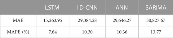
TABLE 6. Comparison of univariate model prediction performance (Rolling forecast).

3.3.2 Multivariate model prediction performance

Furthermore, this paper incorporates a feature analysis of energy data and compares the results of different prediction models considering economic data features only or considering coupled economic and energy data features, as shown in Table 7 below. It is evident that the LSTM model with combined features exhibits superior performance.

TABLE 7

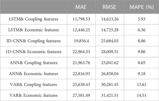
TABLE 7. Comparison of economic feature and coupled feature model prediction performance (Rolling forecast).

3.3.3 Prediction effect of multivariate model combined with wavelet analysis

At the same time, this paper presents an introduction to wavelet analysis and provides a comparative analysis of the outcomes of different prediction models for multi-variable coupled features, as shown in Table 8. It can be seen that for forecasting research related to China’s quarterly GDP, The LSTM&WA model outperforms other deep learning models with notably higher accuracy, such as the 1D-CNN model, machine learning models like the ANN model, and traditional multivariate time series models like the VAR model. Meanwhile, we have confirmed that the inclusion of wavelet analysis in the LSTM&WA model results in significantly improved prediction performance when compared to the LSTM model without wavelet analysis. The introduction of wavelet analysis has improved the LSTM model’s prediction accuracy, such as MAPE, by 0.55%. After determining the model parameters through cross-validation, the LSTM&WA model has stronger generalization ability compared to various benchmark models, and its prediction curve performance is more robust, as seen in Figure 14 Specifically, in the 2019Q3 to 2020Q3 interval, the LSTM&WA model’s predicted values are close to the actual quarterly GDP values, with no significantly abnormal predictions.

TABLE 8

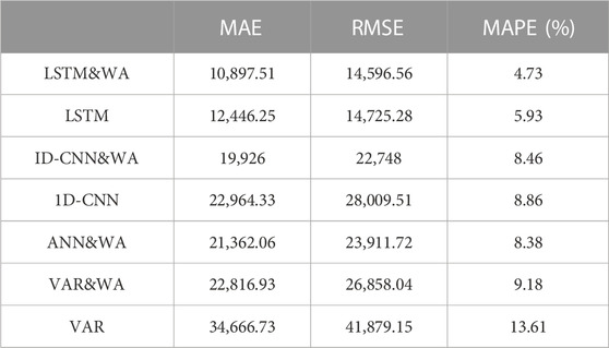
TABLE 8. Comparison of multivariate model prediction performance (Rolling forecast).

FIGURE 14

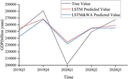
FIGURE 14. LSTM&WA model test set prediction results.

For structurally complex nonlinear multivariable data, the LSTM&WA prediction model exhibits strong generalization capabilities and in terms of prediction accuracy, the LSTM&WA forecast model surpasses the other seven benchmark models (LSTM, 1D-CNN&WA, 1D-CNN, ANN&WA, ANN, VAR&WA, VAR).

In our initial efforts to predict GDP using the LSTM model, we focused solely on economic indicators as input features. Table 7 indicates a prediction error of 6.36%. However, by incorporating energy-related features, we managed to reduce the error to 5.93%. Further enhancement came when we integrated wavelet analysis techniques, leading to a significant accuracy boost. As shown in Table 8, the error decreased to 4.73%, marking a 1.63% improvement from our original rate.

3.4 Computational burden

We believe that incorporating computational efficiency into experimental evaluation is crucial. While accuracy is a key indicator of model performance, the computational time of the model is equally important in real-world application scenarios, as it directly relates to the practicality and operability of the model. We meticulously recorded the overall computational time for model training and forecasting, and compared it with the computational efficiency of other benchmark models in Table 9.

TABLE 9

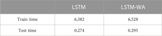
TABLE 9. Time of train and test (s).

We found that despite the higher computational demands of the combined LSTM and WA model in handling time series predictions in Table 9, it exhibits an excellent balance between computational time and forecasting precision in Tables 8, 9, offering a viable and efficient solution for the field of economic forecasting.

4 Conclusion and future work

This research conducts an all-inclusive analysis to scrutinize the relationship between extensive energy data and economic indicators. Furthermore, coupling feature mining of energy big data and economic data is performed to uncover valuable insights, and constructs coupled features of economic data and energy data. In response to the nonlinear change characteristics of China’s quarterly GDP, we introduce the LSTM model from deep learning neural networks and combine wavelet analysis techniques to decompose the selected macroeconomic variables. Subsequently, we construct an LSTM&WA prediction model and conduct prediction research on the high- and low-frequency parts of quarterly GDP. By incorporating wavelet analysis in the feature processing stage, the LSTM neural network model becomes less susceptible to the disruptive influence of short-term noise disturbances. For quarterly GDP data, compared to the LSTM model without wavelet analysis, the LSTM&WA model yields superior prediction outcomes, as evidenced by the prediction accuracy, such as MAPE, increasing by 0.55%.

This paper primarily employs mathematical statistics and data mining knowledge, building models based on related time series data. It does not take into account other factors that may influence China’s GDP. Significant policies or events could potentially cause actual figures to exceed the forecasted range of this paper. Due to limitations in the data sources, data from 2020 and beyond were not utilized, thus, to some extent, avoiding the impact of events like the pandemic. Therefore, for more long-term GDP forecasting, improvements are needed in how to integrate other influencing factors and further refine the model.

Data availability statement

The original contributions presented in the study are included in the article/Supplementary material, further inquiries can be directed to the corresponding author.

Author contributions

YZ: Conceptualization, Data curation, Formal Analysis, Investigation, Methodology, Software, Validation, Writing–original draft, Writing–review and editing. WS: Conceptualization, Formal Analysis, Funding acquisition, Project administration, Resources, Visualization, Writing–review and editing. NZ: Data curation, Validation, Writing–review and editing. XP: Data curation, Validation, Writing–review and editing. BH: Conceptualization, Funding acquisition, Project administration, Supervision, Visualization, Writing–review and editing.

Funding

The author(s) declare financial support was received for the research, authorship, and/or publication of this article. This work was supported by the State Grid Liaoning Electric Power Co., Ltd. Management technology project--Research on macroeconomics and energy consumption forecasting technology based on energy big data (2022YF-113).

Conflict of interest

Authors WS, NZ, and XP were employed by State Grid Liaoning Electric Power Co., Ltd.

The remaining authors declare that the research was conducted in the absence of any commercial or financial relationships that could be construed as a potential conflict of interest.

The authors declare that this study received funding from the State Grid Liaoning Electric Power Co., Ltd.

Management technology project–Research on macroeconomics and energy consumption forecasting technology based on energy big data (2022YF-113). The funder had the following involvement in the study: WS: Conceptualization, Formal Analysis, Funding acquisition, Project administration, Resources, Visualization, Writing–review and editing. NZ: Data curation, Validation, Writing–review and editing. XP: Data curation, Validation, Writing–review and editing.

Publisher’s note

All claims expressed in this article are solely those of the authors and do not necessarily represent those of their affiliated organizations, or those of the publisher, the editors and the reviewers. Any product that may be evaluated in this article, or claim that may be made by its manufacturer, is not guaranteed or endorsed by the publisher.

References

Altinay, G., and Karagol, E. Electricity consumption and economic growth: evidence from Turkey. Energy Econ., 2005, 27(6): 849–856. doi:10.1016/j.eneco.2005.07.002

CrossRef Full Text | Google Scholar

Ashraf, Z., Javid, A. Y., and Javid, M. 2013 Electricity consumption and economic growth: evidence from Pakistan. Econ. Bus. Lett., 2(1): 21–32. doi:10.17811/ebl.2.1.2013.21-32

CrossRef Full Text | Google Scholar

Box, G. E., and Jenkins, G. M. Time series analysis: forecasting and control. J. Time, 2010, 31(3). doi:10.1111/j.1467-9892.2009.00643.x

CrossRef Full Text | Google Scholar

Das, A., Chowdhury, M., and Khan, S. (2012). The dynamics of electricity consumption and growth nexus: empirical evidence from three developing regions. J. Appl. Econ. Res. 6 (4), 445–466. doi:10.1177/0973801012462121

CrossRef Full Text | Google Scholar

Dickey, D. A., Hasza, D. P., and Fuller, W. A. (1984). Testing for unit roots in seasonal time series. J. Am. Stat. Assoc. 79 (386), 355–367. doi:10.1080/01621459.1984.10478057

CrossRef Full Text | Google Scholar

Ferguson, R., Wilkinson, W., and Hill, R. Electricity use and economic development. Energy Policy, 28. (2000):923–934. doi:10.1016/s0301-4215(00)00081-1

CrossRef Full Text | Google Scholar

Huang, B., Li, Y., Zhan, F., Sun, Q., and Zhang, H. (2022). A distributed robust economic Dispatch Strategy for integrated energy system considering cyber-attacks. IEEE Trans. Industrial Inf. 18 (2022), 880–890. doi:10.1109/tii.2021.3077509

CrossRef Full Text | Google Scholar

Huang, B., Wang, Y., Yang, C., Li, Y., and Sun, Q. A neurodynamic-based distributed energy management approach for integrated local energy systems. Int. J. Electr. Power & Energy Syst., 2021, 128(PT.1-1082):106737. doi:10.1016/j.ijepes.2020.106737

CrossRef Full Text | Google Scholar

Kingma, D. P., and Ba, J. (2014). Adam: a method for stochastic optimization. Comput. Sci. doi:10.48550/arXiv.1412.6980

CrossRef Full Text | Google Scholar

Kraft, J., and Kraft, A. Relationship between energy and GNP. J. Energy Finance Dev., 1978, 3:(2):401–403. doi:10.1016/0301-4215(78)90010-1

CrossRef Full Text | Google Scholar

Debenedictis, L. F. A vector autoregressive model of the British Columbia regional economy. Appl. Econ., 1997. doi:10.1080/000368497326534

CrossRef Full Text | Google Scholar

Liu, Z., Huang, B., Hu, X., Du, P., and Sun, Q. (2023). Blockchain-based renewable energy trading using information entropy theory. IEEE Trans. Netw. Sci. Eng., 1–12. doi:10.1109/TNSE.2023.3238110

CrossRef Full Text | Google Scholar

Liu, Z., Xu, Y., Zhang, C., Elahi, H., and Zhou, X. (2022). A blockchain-based trustworthy collaborative power trading scheme for 5G-enabled social internet of vehicles. Digital Commun. Netw. 8 (6), 976–983. doi:10.1016/j.dcan.2022.10.014

CrossRef Full Text | Google Scholar

Ngungu, M. M., Noah, W., and Noah, W. (2018). Modeling agricultural gross domestic product of Kenyan economy using time series. Asian J. Probab. Statistics, 1–12. doi:10.9734/ajpas/2018/v2i124563

CrossRef Full Text | Google Scholar

Stern, D. I. A multivariate cointegration analysis of the role of energy in the US macroeconomy [J], Energy Econ., 22(2000):267–283. doi:10.1016/s0140-9883(99)00028-6

CrossRef Full Text | Google Scholar

Tan, M., Hu, C., Chen, J., Wang, L., and Li, Z. (2022). Multi-node load forecasting based on multi-task learning with modal feature extraction. Eng. Appl. Artif. Intell. 112, 104856, 104856. doi:10.1016/j.engappai.2022.104856

CrossRef Full Text | Google Scholar

Tkacz, G. Neural network forecasting of Canadian GDP growth. Int. J. Forecast., 2001, 17, 57, 69. doi:10.1016/s0169-2070(00)00063-7

CrossRef Full Text | Google Scholar

Wu, X., Zhang, Z., Chang, H., and Huang, Q. (2021). A data-driven gross domestic product forecasting model based on multi-indicator assessment. IEEE Access 9, 99495–99503. doi:10.1109/access.2021.3062671

CrossRef Full Text | Google Scholar

Yan, K., Li, W., Ji, Z., Qi, M., and Du, Y. (2019). A hybrid LSTM neural network for energy consumption forecasting of individual households. IEEE Access 7, 157633–157642. doi:10.1109/access.2019.2949065

CrossRef Full Text | Google Scholar