 Yonghui Duan
 Jianhui Zhang
 Xiang Wang2
- 1Department of Civil Engineering, Henan University of Technology, Zhengzhou, China
- 2Department of Civil Engineering, Zhengzhou University of Aeronautics, Zhengzhou, China
As a clean fossil energy source, natural gas plays a crucial role in the global energy transition. Forecasting natural gas prices is an important area of research. This paper aims at developing a novel hybrid model that contributes to the prediction of natural gas prices. We develop a novel hybrid model that combines the “Decomposition Algorithm” (CEEMDAN), “Ensemble Algorithm” (Bagging), “Optimization Algorithm” (HHO), and “Forecasting model” (SVR). The hybrid model is used for monthly Henry Hub natural gas forecasting. To avoid the problem of data leakage caused by decomposing the whole time series, we propose a rolling decomposition algorithm. In addition, we analyzed the factors affecting Henry Hub natural gas prices for multivariate forecasting. Experimental results indicate that the proposed model is more effective than the traditional model at predicting natural gas prices.
1 Introduction
The use of energy is a crucial part of production and consumption processes in all industries. A reliable, affordable, and stable energy supply is essential for industrial production, transportation, home heating, and commercial production. With the growth of the global population and the acceleration of industrialization, energy demand continues to increase, which results in a more complex and competitive energy market (Wang et al., 2021). In the area of data analysis and forecasting, energy price forecasting has received a lot of attention. Accurate energy price forecasts are of great benefit to researchers and policymakers.
As the demand for energy grows, environmental issues resulting from high emissions and pollution from fossil fuels are becoming more serious. The transition to renewable energy has become an urgent issue. Clean energy development and utilization are gradually attracting worldwide attention (Dong et al., 2022). As a low-carbon and clean energy source among fossil fuels, natural gas plays a crucial interim role in the transition to a sustainable energy economy (Rabbi et al., 2022).
To formulate rational energy policies, it is essential to make accurate predictions of natural gas price trends. They also optimize market operations, sustainable economic development, and global energy transition promotion.
Currently, the North American market, the UK market, and the Japanese and Korean markets are dominating the international natural gas market. The price trends of Henry Hub in the North American market, NBP at the Intercontinental Exchange (ICE) in the European market, and Platts Japan LNG import prices in the Asian market have become essential reference indicators for assessing international natural gas price levels (Geng et al., 2016). Among them, the Henry Hub market is the most liquid, volatile, and unpredictable natural gas market. Research on natural gas price forecasting in the Henry Hub is important due to its importance in natural gas trading, power production planning, and regulatory decisions.
In this paper, the major research purpose is to propose a novel hybrid model to predict natural gas prices more accurately. We constructed a model combining Harris hawks optimization (HHO), Bagging integrated learning, support vector regression (SVR), and complete ensemble empirical mode decomposition with adaptive noise (CEEMDAN). There are many studies about “Decomposition Algorithm” + “Forecasting Model” and “Ensemble Algorithm” + “Forecasting Model.” However, few studies combine the “Decomposition Algorithm,” “Ensemble Algorithm,” “Optimization Algorithm,” and “Forecasting Model.” We conducted this experiment and verified its feasibility.
First, the SVR model is optimized using the HHO algorithm to reduce subjectivity of the parameter settings and improve prediction accuracy, then the Bagging integration strategy is applied to the HHO–SVR model to further enhance model performance, and the Bagging–HHO–SVR model is constructed. A CEEMDAN algorithm was used to decompose natural gas price monthly time series into multiple modal components. The CEEMDAN–Bagging–HHO–SVR prediction model reduces the subjectivity and complex parameter setting of the SVR model. While reducing the variance of the model, it also optimizes the impact of noise on time series data, allowing it to extract the inherent features of the data. When applying CEEMDAN to decompose data, we adopted a rolling decomposition method to avoid the potential problem of data leakage caused by previous methods. The final experimental results indicate that the constructed model has a high level of prediction accuracy and relatively stable performance.
In summary, this paper makes several major contributions:
(1) To better predict the Henry Hub natural gas price, we integrated “Decomposition Algorithm” + “Ensemble Algorithm” + “Optimization Algorithm” + “Forecasting Model” based on machine learning technology and proposed a novel hybrid prediction model.
(2) We improved the way CEEMDAN works on datasets in the past and adopted a rolling decomposition approach. This method can avoid data leakage.
(3) We took into account the external influencing factors of Henry Hub natural gas prices in the input variables, which further improves the prediction accuracy and stability of the model.
(4) In order to understand the model and which features have the greatest impact on the prediction results of the model, we conducted a feature importance analysis. In addition, we identified significant factors that affect Henry Hub natural gas prices.
The structure of the rest of this paper is as follows: Section 2 is a literature review. Section 3 describes algorithms and models. Section 4 describes the data preparation work, prediction process, and variable screening experiments. Section 5 discusses the data description and experimental results. Section 6 summarizes some conclusions and proposes some suggestions.
2 Literature review
Energy forecasting typically spans different prediction horizons, including short term (hours and days), medium term (weeks), and long term (months and years). As a result of the different prediction ranges, the sample size varies as well. The sample size of daily predictions is usually larger than that of monthly predictions (Arvanitidis et al., 2022), and natural gas price forecasting focuses on daily, weekly, and monthly forecasts. This paper focuses on the monthly price forecast, which is a small sample size for long-term price forecasting. Therefore, this paper chooses the SVR model, which is excellent for small-sample quantity prediction, and compares it to the other benchmarking models.
Additionally, energy price predictions can be classified into univariate and multivariate predictions according to the variables involved (Hou et al., 2022). Most previous studies on natural gas prices have used univariate forecasts. In univariate forecasting, only historical natural gas price data are introduced as input variables into the forecasting model. This forecasting method assumes that external factors are stable, which saves time and effort collecting relevant influencing factors. However, the drawback is that some critical factors are often overlooked, and the forecasting model is not comprehensive enough. This usually results in relatively limited forecasting accuracy. Multivariate forecasting incorporates a variety of other factors that affect changes in natural gas prices. This method can make input variables more comprehensive, although it takes more time and effort to collect and process data. In this paper, we consider and use grey relation analysis (GRA) to examine multiple factors that influence natural gas price changes. In order to improve the quality of input variables, retained factors will be used in conjunction with historical natural gas prices as input variables.
The available literature indicates that energy forecasting models can broadly be categorized into traditional economic models and machine learning models based on artificial intelligence (Lu et al., 2021). Particularly in recent years, as artificial intelligence has seen rapid advancements, more studies have employed machine learning models. Econometric models, which are based on economic principles and statistical methods, build mathematical models to make predictions. Common econometric models include time series models (e.g., autoregressive moving average (ARMA), generalized autoregressive conditional heteroskedasticity (GARCH), and autoregressive integrated moving average (ARIMA)) (Ma and Wang, 2019; Son et al., 2020; Zhang et al., 2021; Sun et al., 2023) and regression models (e.g., multiple linear regression (MLR) and vector autoregression (VAR)) (Youssef et al., 2021; Egbueri J and Agbasi J., 2022; Pannakkong et al., 2022). Although these models can capture trends, seasonality, and periodicity in price series, they are less capable of addressing nonlinear problems and large-scale datasets. Moreover, energy forecasting is usually based on irregular and nonlinear data in real life. Yu and Yang (2022) used China’s electricity demand dataset spanning from 2004 to 2019. They combined the dataset with the ARMA model, to analyze the future electricity situation in China and accurately predict China’s electricity demand in 2020. Alam et al. (2023) used the ARIMA model to predict coal, oil, and natural gas prices in India before and after COVID-19. The empirical results suggest that the ARIMA model is appropriate for forecasting coal, crude oil, and natural gas prices in India. Hou and Nguyen (2018) applied a Markov switching vector autoregressive model (MS-VAR) to examine the institutional response patterns of the natural gas market to underlying fundamental shocks. Their study identified the presence of four separate regimes within the American natural gas market. Nguyen and Nabney. (2010) first proposed an adaptive multilayer perceptron (MLP)/GARCH model combined with wavelet transform (WT) to predict electricity demand and natural gas prices in the UK, achieving high prediction accuracy.
Comparatively, machine learning models make predictions by learning patterns and regularities from historical data. Over the past few years, significant progress has been made in energy forecasting to address the shortcomings of traditional econometric models. Typical machine learning models encompass SVR models (Jianwei et al., 2019), neural network models (Wang et al., 2020), and decision tree models (Yahşi et al., 2019; Bentéjac et al., 2020). These models have strong nonlinear modeling capabilities, can handle large-scale datasets, and can automatically extract features from the data to better capture complex relationships in energy prediction. Since machine learning models often have many parameters to be set, these parameters significantly impact the predictive performance of the model. Moreover, manual parameter setting involves subjectivity and costs a lot of time. Intelligent optimization algorithms can automatically search the large-scale parameter space and find the best solution. Ma et al. (2019) used grey wolf optimization combined with a novel fractional time-delayed grey model to predict natural gas and coal consumption in Chongqing, China. The results suggest that the optimized model of grey wolf optimization outperforms the rest of the comparative models. Zhu et al. (2023) optimized the model constructed in the paper with the marine predator algorithm and enhanced forecasting performance. Essa et al. (2020) improved the prediction accuracy of conventional artificial neural networks by optimizing their parameters using Harris hawks optimization.
Machine learning models are categorized into single and hybrid models. Single models use only one machine learning algorithm or model for natural gas price forecasting. These models generally focus on a specific algorithm or model structure and are trained on data to obtain predictions. Čeperić et al. (2017) used an SVR model and a feature selection method to forecast Henry Hub natural gas spot prices. Salehnia et al. (2013) used a calibrated ANN model to predict the Henry Hub natural gas price with the help of the gamma test. Zhang and Hamori (2020) integrated the dynamic moving window method with the XGBoost model to forecast the U.S. natural gas crisis.
A single model cannot achieve continuous satisfactory prediction performance when dealing with various data and is prone to ignoring the internal characteristics of the data or overfitting, which means most of them have limitations (Yu et al., 2021; Zhang et al., 2022). The hybrid model refers to the combination of multiple machine learning algorithms or models to achieve better performance and generalization ability. According to previous literature, the prediction performance of the hybrid model is always better than that of the economic model and the single model (Jiang et al., 2022a).
Jung et al. (2020) constructed a hybrid model by combining “bagging” algorithms with “multilayer perceptron.” The final result analysis shows superior performance. Meira et al. (2022) proposed a novel generalization algorithm by combining the Bagging integration method with a modified regularization technique. The study constructed a novel hybrid model and empirically analyzed monthly natural gas consumption in 18 European countries. Li et al. (2021) constructed a VMD–PSO–DBN model using the VMD algorithm combined with the PSO-optimized DBN model to empirically analyze monthly natural gas prices in Henry Hub. The results suggested that the newly constructed model predicted better than traditional models. Fang et al. (2023) combined EMD with ISBM–FNN and developed an EMD–ISBM–FNN model to decompose and predict crude oil prices. To verify the model’s prediction results, a comparison scheme was designed to compare the results. Results indicate that the model had the highest prediction results and outperformed previous research. Zhan et al. (2022) proposed a technique combining LSTM and quadratic decomposition to construct an improved natural gas forecasting hybrid model VMD–EEMD–Res.–LSTM and then selected the monthly natural gas spot price of Henry Hub for empirical analysis. Wang et al. (2022) combined the decomposition algorithm with the multi-objective grasshopper optimization algorithm, and used nine models to predict the decomposed components. Then, they conducted short-term power load forecasting, ultimately achieving satisfactory results in point and interval prediction.
3 Methodology
3.1 Support vector regression
Support vector machine (SVM) was proposed by Cortes and Vapnik for classification tasks (Cherkassky, 1997). Later, SVR was developed based on the SVM. SVR relies on the principle of structural risk minimization, which makes it ideal for solving high-dimensional, small-sample nonlinear problems. Its primary purpose is to convert a nonlinear regression problem with a low dimension into a linear regression problem with a high dimension (Zheng et al., 2023). Based on dataset
where W and b denote the weight coefficient and bias term (Cai et al., 2023).
The constraints are
where
Subsequently, the Lagrange multipliers are introduced
where
where
3.2 Grey wolf optimization algorithm
The grey wolf optimizer (GWO) is a swarm intelligence optimization algorithm proposed in 2014 by Mirjalili et al. (2014), who are scholars from Griffith University, Australia. The algorithm has a simple structure, high convergence, and no excessive parameter settings. The GWO algorithm simulates the leadership hierarchy and hunting mechanisms of grey wolves in nature based on their predatory behavior. It classifies grey wolves into four types. The algorithm consists of three main parts: surrounding the prey, approaching the prey, and attacking the prey.
In the GWO algorithm, four wolves are established with varying social ranks, including α, β, δ, and ω. Among them, α simulates the head wolf (level 1 wolf), which leads the entire grey wolf pack and is responsible for leading the whole pack to hunt for prey. α represents the optimal solution to the problem. β is the level 2 wolf, which is responsible for assisting α. δ is the level 3 wolf, which obeys the commands and decisions of α and β, and is responsible for scouting and standing guard. ω is the level 4 wolf, which is located at the bottom of the entire hierarchy. It obeys the commands from the former level 3 wolf to carry out the position around α, β, or δ update (Liu Z et al., 2023).
(1) Surrounding the prey
The GWO algorithm uses the following formula to encircle its prey before hunting:
where
(2) Approaching the prey
The formulas of
where
(3) Attacking the prey
Grey wolves are expected to begin hunting behavior after identifying the approaching prey. The hunting behavior is generally led by the α-wolf, assisted by the β-wolf and δ-wolf, and ω-wolf update based on their position. The mathematical formula for hunting is as follows:
where
where
3.3 Marine predator optimization algorithm
Faramarzi et al. (2020) proposed the marine predators algorithm (MPA) in 2020. The algorithm is primarily inspired by foraging behavior in marine predators. Essentially, this involves the Lévy and Brownian movements of marine predators and the optimization of the encounter rate strategy between the predators and prey. It is based on the theory of survival of the fittest in the ocean. The MPA has high optimization search performance. Among them, the Brownian motion search step is large enough to track and explore neighboring regions to achieve global optimization. In contrast, the Lévy motion search step is small enough to effectively explore local regions in depth to achieve local optimization. There are three main phases to the algorithm: the pre-search phase, the mid-search phase, and the post-search phase.
(1) Pre-search phase
During the phase of pre-search, we assume that the prey will move faster than the predator, at which point the predator should remain stationary.
When Iter <
where
(2) Mid-search phase
In the mid-search stage, we assume that both the predator and the prey are moving at the same speed. During this phase, the predator simulates the hunt for the prey, while the prey, as a potential predator, searches for a prey of a lower rank than itself. At this point, the prey exploits in accordance with a Lévy wandering strategy, while the predator explores in accordance with a Brownian wandering strategy and gradually transitions from an exploration strategy to an exploitation strategy.
When
where
When
where CF =
(3) Post-search phase
At this stage, we assume that the predator has a higher speed compared to the prey, at which point the predator’s best strategy is Lévy movement.
When Iter >
(4) Addressing vortex effects and FAD effects
Moreover, the algorithm takes into account environmental factors affecting marine predators’ behavior to avoid the algorithm converging prematurely, for example, eddy current effects and fish aggregating device (FAD) effects. The mathematical formulation is as follows:
where FADs = 0.2 is a fixed value indicating the probability that a predator is affected by FADs.
(5) Marine memory
The purpose of this step is to update the elite matrix which is the optimal fitness value. After updating the prey matrix, the fitness value of each prey in the matrix is calculated. If it is better than the fitness value of the corresponding position in the elite matrix, it is replaced. Then, the optimal individual fitness value for the elite matrix is calculated.
3.4 Harris hawks optimization algorithm
Heidari et al. (2019) first proposed the HHO algorithm in 2019. The algorithm has strong global search capability and converges quickly with fewer parameters to tune. The algorithm is inspired by the Harris hawk’s prey capture process. This process can dynamically adjust its prey capture strategy by considering the dynamic nature of the environment and the prey’s escape patterns. The algorithm consists of three main phases: search, conversion between search and exploitation, and exploitation. Figure 1 shows the flowchart of the Harris hawks algorithm.
(1) Search phase
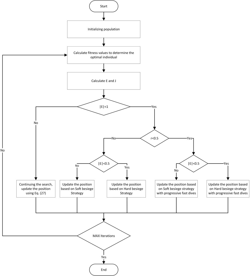
FIGURE 1. Flowchart of the Harris hawks algorithm.
The Harris hawk searches and follows its prey with keen eyes. Considering that the prey is not easy to detect, the authors designed two strategies to simulate the Harris hawk’s prey capture.
where
where M denotes the population size.
(2) Conversion phase of search and exploitation
In the HHO algorithm, it is assumed that prey escape consumes escape energy. Harris hawk can shift between different exploitation behaviors according to the prey’s escape energy. Escape energy is defined as
where E is the escape energy of the prey.
(3) Exploitation phase
After entering the exploitation phase, hawks will dynamically adopt a capture strategy based on the real-time state of their prey. To choose a strategy, a random number r between [0,1] is defined.
(1) Soft besiege strategy
When
where
(2) Hard besiege strategy
When
(3) Soft besiege strategy with progressive fast dives
When r < 0.5 and
where
where Γ is the gamma function, u and v are D-dimensional random vectors in [0,1], and β is a default value set to 1.5.
(4) Hard besiege strategy with progressive fast dives
When r < 0.5 and
where Y and Z are updated and are obtained from Eq. 39 and Eq. 40, respectively.
3.5 Bagging integration algorithm
Ensemble learning is a method that can improve generalization performance significantly than a single learner by combining multiple learners. There are many integration algorithms including Boosting, Stacking, and Bagging. In this paper, the Bagging integration learning algorithm is used. The Bagging algorithm (Boostrap aggregation) is a widely used machine learning technique (Breiman, 1996). The idea is to improve the entire learner’s generalization ability by combining multiple homogeneous learners’ results. The Bagging algorithm has the capability to enhance accuracy and stability and prevent overfitting when combined with multiple models.
Bagging is suitable for small-sample problems. It is possible to significantly reduce the variance in the model training process by using a subset of the dataset and averaging the results, as well as mitigate the problem of overfitting. Boosting is appropriate for weak learners as it reduces bias. Its training process is serial, which requires training the base classifiers and updating the weights one by one, which can make overfitting a possibility for some problems. Stacking’s training process is relatively complex, requiring the training of multiple models and the fusion of predictions, which increases training time and computational cost. It may also lead to overfitting when the training data are small or the model complexity is high. As the HHO–SVR model is better suited for reducing variance than bias and our dataset is a small sample, Bagging algorithms are more appropriate for this study (Zounemat-Kermani et al., 2021; Mienye and Sun et al., 2022).
By using random sampling with dropouts from the original dataset, multiple subsets of the original dataset that have the same size are extracted from the original dataset. Base learners are trained independently using each subset. Finally, when performing regression predictions, the Bagging algorithm sums up all predictions and averages them in order to arrive at the final prediction.
3.6 Complete ensemble empirical mode decomposition with adaptive noise
EEMD and CEEMD aim to alleviate mode aliasing associated with EMD decomposition due to mode aliasing. They achieve this by introducing pairwise Gaussian white noise with opposite phases to the original signal. Nevertheless, despite these efforts, both algorithms may still retain some residual white noise after signal decomposition, which can impact the accuracy of subsequent decomposition processes. Torres et al. (2011) proposed a novel signal decomposition algorithm CEEMDAN. As part of EEMD (Wu and Huang, 2009), the algorithm averages the components immediately after adding fixed white noise to the original signal and performing the EMD decomposition. CEEMDAN adds adaptive white noise to the residual terms after each order of components and averages the components. Therefore, CEEMDAN has better decomposition performance and denoising ability compared to EEMD. The following are the decomposition steps:
(1) The Kth Gaussian white noise is added to the original signal to be decomposed, and a new signal is constructed.
where
(2) On each new signal obtained, EMD decomposition is performed to obtain K components. Then, the K components are summed and averaged to obtain the first-order modal components from the CEEMDAN decomposition.
where
(3) We continue to add the Gaussian white noise to the above residual term
The EMD decomposition is performed again on the new signal to obtain K components, which we sum and average to produce the second-order modal components obtained from the CEEMDAN decomposition:
where
(4) These steps are repeated until the residual term becomes a monotonic function that cannot be further decomposed. Finally, the original signal is decomposed into j modal components and one residual term with the following mathematical formula:
After obtaining the components and residual terms derived from the CEEMDAN decomposition, appropriate prediction models can be used to forecast each component. Finally, the forecasting results are linearly summated to obtain the final results. In this paper, the optimal model in the comparison was used to predict components.
4 Henry Hub natural gas price prediction process and variable screening
4.1 Data preprocessing
(1) Data difference
The drastic volatility of the raw data will have an impact on the model’s prediction. A data difference can eliminate some of the fluctuations and improve the smoothness of the data. The mathematical principle is relatively simple, subtracting the previous value from the next value to get a difference value. The formula is as follows:
where
(2) Data normalization
Data normalization is often used in machine learning preprocessing. When features in the dataset exhibit varying value ranges, data normalization becomes crucial. Data normalization aims to standardize features on the same metric scale, to facilitate prediction and improve prediction accuracy. Therefore, the min–max normalization method is used to normalize the dataset so that all data sizes are between [0,1]. Its mathematical formula is as follows:
where
4.2 Parameter setting
In this paper, we selected a variety of models for multi-level comparisons. Among the single models, we selected persistence, ARIMA, back-propagation neural network (BPNN), extreme learning machine (ELM), XGBoost, and SVR models. Among the optimization algorithms, we chose GWO, MPA, and HHO optimal algorithms. For the ensemble algorithm, we selected the Bagging algorithm. For the decomposition algorithm, we chose EEMD, VMD, and CEEMDAN algorithms. In the following, we explained some of the algorithms that require parameter setting.
The ARIMA model is the most commonly used econometric model. The main parameters of this model are (p, d, q), where d is determined by the ADF test, and p and q are determined by the AIC and BIC values (Kaur et al., 2023), respectively. We determined (p, d, q) = (2,0,1) by using the ADF test and BIC values. One of the most widely used neural network models is the BPNN, which consists of three layers: the input layer, the hidden layer, and the output layer. The number of neurons in its hidden layer is very important, usually depending on the size and dimension of the dataset, and there is no fixed selection method (Wang et al., 2020). We chose a hidden layer consisting of 32 neurons in this paper. The ELM is a single hidden layer feed-forward neural network that does not require iteration. Similar to other neural networks, the number of neurons in the hidden layer has a significant effect (Chaudhuri and Alkan B., 2021; Jiang et al., 2022b). We set up a single hidden layer with 12 neurons based on the data in this paper and randomly initialized hidden weights and biases. XGBoost has been a popular gradient boosting model in recent years. Because it is used as a benchmark experiment in this paper, its parameters are the defaults. To facilitate comparisons, the SVR model uses default parameters from the benchmark model. The forecasting performance of SVR is mainly affected by C and gamma (Ngo N et al., 2022), so we used optimization algorithms to optimize these two parameters. Based on previous literature and the performance of the three optimization algorithms in this paper, for fairness, we have the same settings for all three algorithms (Lu et al., 2022; Mohammed S et al., 2022; Sharma and Shekhawat et al., 2022; Su X et al., 2022): iterations: 30; population: 20; and lower and upper bound [0.1,1]. In the Bagging algorithm, the main factors that affect its performance include base learners and data samples (Mohammed and Kora et al., 2023). Data samples and the type of base learners were determined in this paper. Therefore, the parameters that need to be manually set in the Bagging algorithm are mainly the number of base learners. Based on the test results of the experiment, we set the number of base learners to 15. The VMD algorithm is mainly influenced by the decomposition modes K and the central frequency bandwidth α impact. The residual increases as α increases, and the larger the K value, the more the components generated by decomposition, which may lead to overdecomposition (Pei Y et al., 2022). We set k = 5, α = 200. We list more detailed parameter settings in Table 1.
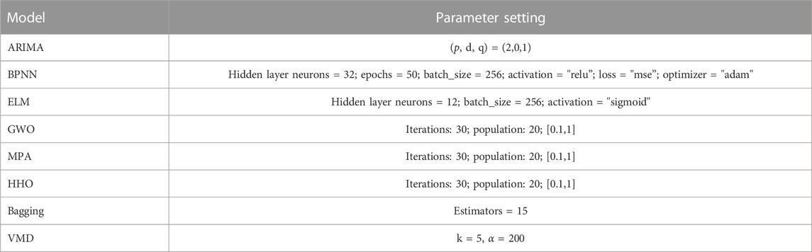
TABLE 1. Model parameter settings.
4.3 Henry Hub natural gas price prediction process
In this paper, we used CEEMDAN to decompose Henry Hub natural gas prices. The HHO algorithm was selected for SVR model parameter optimization, and the Bagging algorithm was used for ensemble learning of the HHO–SVR model. The final prediction model CEEMDAN–Bagging–HHO–SVR hybrid prediction model was constructed. Due to the fact that multi-steps ahead prediction can better mine the unique information contained in historical data, based on the experience of previous literature, we used a three-step ahead prediction method, which selects data from days t-1, t-2, and t-3 as input variables to predict data from day t (Zhang et al., 2021; Wang et al., 2023).
Specifically, the CEEMDAN decomposition method in previous literature usually directly decomposes the entire time series, including the training set and test set. After obtaining the components, each one is predicted separately, and finally, they are summed in order to obtain the predicted value. Due to the fact that the test set belongs to future data, data leakage will occur when all test sets are unknown and training sets are decomposed simultaneously (Qian Z et al., 2019; Gao R et al., 2021). We made improvements to this problem by gradually decomposing and predicting time series using a rolling approach. The process is as follows.
First, the CEEMDAN decomposition is performed on the entire training set and then one step backward is predicted to obtain the first predicted value.
Next, the training set is extended backward by one data point, CEEMDAN decomposition is performed on the new training set, and another backward prediction step is made to obtain the second predicted value.
…….
These steps are repeated until all predicted values are obtained.
For the convenience of comparison, we retained the previous decomposition method for EEMD and VMD and only used the rolling decomposition method for CEEMDAN.
In the following, we provide a detailed introduction to the process of combining rolling decomposition with the Bagging algorithm, HHO algorithm, and SVR. This is the entire prediction process.
(1) The eight screened influencing factors together with the historical natural gas price data were used as input variables to compose the input dataset.
(2) Data preprocessing work such as data difference and normalization was performed on the input dataset. This can unify data standards and improve data quality and prediction accuracy.
(3) The processed dataset was divided into training and testing sets, with a ratio of 8:2 between the training and testing sets.
(4) CEEMDAN decomposition was performed on the current training set to obtain six modal components. Each component was randomly sampled into n subsets as an input dataset for the Bagging algorithm.
(5) n subsets were input into the HHO algorithm for parameter optimization to obtain the optimal parameters. The optimized parameters were input into the corresponding SVR model for each subset separately.
(6) n subsets were independently predicted using n SVR models, predicting only one step backward at a time. The arithmetic average of n prediction results was calculated to obtain the predicted value of one component. Finally, the prediction values of the six components were summed to obtain the final single predicted value.
(7) The training set was extended one step backward to obtain a new training set. Steps 4–6 were repeated to obtain other predicted values.
In the above steps, steps 4–6 include the combination process of the Bagging algorithm, HHO algorithm, and SVR. Figure 2 more intuitively shows the combination process of Bagging, HHO, and SVR. Rolling decomposition prediction is mainly carried out in step 7, and Figure 3 shows this process more intuitively.

FIGURE 2. Flowchart of Bagging–HHO–SVR.

FIGURE 3. Flowchart of rolling decomposition.
4.4 Variable screening
4.4.1 Initial variable selection
Natural gas price prediction is affected by numerous complex external factors besides historical natural gas price data. Li et al. (2017) analyzed 20 variables affecting Henry Hub’s natural gas prices using factor analysis and found that natural gas demand and economic conditions were more prominent. Stajic et al. (2021) employed multiple linear regression to analyze the critical drivers of global natural gas price volatility. According to their analysis, natural gas prices are robustly correlated with factors such as crude oil prices and natural gas production. Li et al. (2019) investigated the correlation between Henry Hub natural gas prices and WTI crude oil prices through a multi-scale perspective. Zheng et al. (2023) used the feature select algorithm to screen 20 variables affecting natural gas prices. It found that natural gas drilling activities and natural gas import and export prices had the most impact. Azadeh et al. (2012) validated their hybrid model for enhanced natural gas price forecasting in the industrial sector, utilizing input variables such as natural gas consumption, CPI, and GDP. Su et al. (2019) used machine learning on Henry Hub natural gas prices by considering factors such as temperature and heating oil prices as input variables and finally obtained better prediction results.
The choice of input variables significantly influences the forecasting performance of the constructed model. We used the literature analysis method to select 14 external influence factors on natural gas prices from four aspects initially in this paper. These factors included economic indicators, natural gas market, and climatic factors. Table 2 shows the 14 influence factors with the historical natural gas price. Table 3 shows descriptive statistics for all variables we initially selected.
(1) Economic indicators
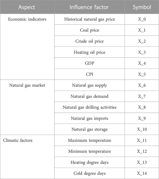
TABLE 2. Variables selected initially.
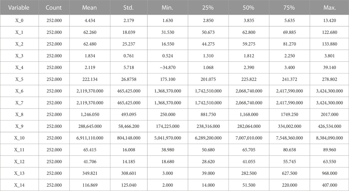
TABLE 3. Descriptive statistics of variables.
Concurrently, overall economic performance and inflation levels also directly or indirectly affect natural gas supply and demand dynamics, subsequently influencing its price. GDP and CPI are primary indicators reflecting a country’s economic status and need to be considered comprehensively among the factors affecting natural gas prices. Energy prices and economic indicators are significantly correlated. Natural gas, as a cleaner energy source, is directly influenced by factors such as coal prices, crude oil prices, and heating oil prices, and when prices of other energy sources rise, businesses and consumers may seek to use natural gas as an alternative energy source, thereby increasing its demand and driving up its price. Therefore, when analyzing the fluctuations and trends in natural gas prices, these economic indicators and related energy price factors must be taken into account. Preliminarily, we selected GDP, CPI, coal prices, heating oil prices, and crude oil prices as factors in economic indicators in this paper.
(2) Natural gas market
Supply and demand are the major factors determining commodity prices. Therefore, the balance of supply and demand is critical to maintaining stable natural gas prices. Natural gas drilling and production activities directly influence the supply of natural gas, which plays a significant role in determining the price of natural gas. In addition, natural gas import and storage have a direct or indirect impact on natural gas supply and demand. Preliminarily, we selected natural gas supply and demand, natural gas drilling activities, natural gas imports, and natural gas storage as factors in the natural gas market in this paper.
(3) Climatic factor
Due to the seasonal nature of natural gas, temperature and climate changes will have a direct impact on the seasonal demand for natural gas, the stability of the supply chain, and the storage requirements, which will in turn impact the price of natural gas. Preliminarily, we selected the maximum temperature and the minimum temperature and heating degree days (HHDs) and cold degree days (CCDs) as factors in this paper.
4.4.2 Grey relation analysis
As a result of the preliminary selection of variables, it is necessary to further screen them to determine which variables have a higher correlation with Henry Hub natural gas prices to reduce the subjectivity of the input variables and improve prediction accuracy. Using the 14 variables selected initially in this paper, we conducted a GRA on natural gas prices and ultimately identified eight external influencing factors as input variables to the model along with historical natural gas prices. GRA is a method for conducting system analysis and determining the importance of factors that affect the development of the system (Arce et al., 2015). The basic idea is to establish a reference sequence that changes over time according to certain rules. Then, we need to treat each influence factor as an analysis sequence and compute the correlation between each analysis sequence and the reference sequence. A higher correlation indicates a stronger relationship between the reference sequence and the analysis sequence. The specific flow of the algorithm is as follows:
(1) Determination of analysis and reference sequences
The natural gas price data are taken as the reference sequence
(2) Programmability
Since the individual factor columns in the analysis series may be inconvenient to compare due to different magnitudes, this paper adopts the min–max method to perform dimensionless operations on the above series.
(3) Grey relation calculation
The correlation coefficient is calculated between each analysis sequence and reference sequence separately. The mathematical formula is
where
(4) Average correlation coefficient
The correlation coefficient is the level of correlation between the analysis sequence and the reference sequence at different time points. It is necessary to concentrate them into a final value (average them) to facilitate holistic comparisons. The mathematical formula is as follows:
where
Table 4 shows the grey correlation between natural gas price and the remaining 14 variables in this paper. A grey correlation less than 0.7 indicates a low correlation between the series. So, this paper eliminates the grey correlations less than 0.7 and filters out the final eight variables that will be used together with the Henry Hub historical natural gas price as input variables.
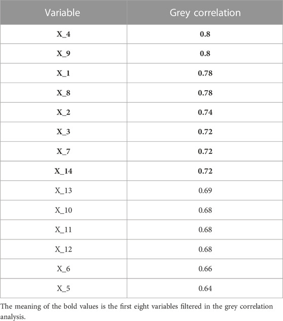
TABLE 4. Grey correlation ranking of variables.
5 Empirical analysis and discussion
5.1 Data description
Historical Henry Hub natural gas price data, coal price data, crude oil price data, heating oil price data, natural gas demand data, natural gas drilling activities data, and natural gas import data were acquired from the U.S. Energy Information Administration website (https://www.eia.gov). The GDP data were acquired from the U.S. Bureau of Economic Analysis website (https://www.bea.gov). The CDD data were acquired from the National Oceanic and Atmospheric Administration website (https://www.ncdc.noaa.gov). Table 5 describes variables in detail. All of the above data are monthly data from January 2001 to December 2021, totaling 252 data. Figure 4 shows the strong volatility and nonlinear characteristics of the natural gas price data.
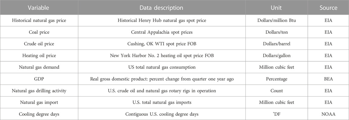
TABLE 5. Details of input variables.
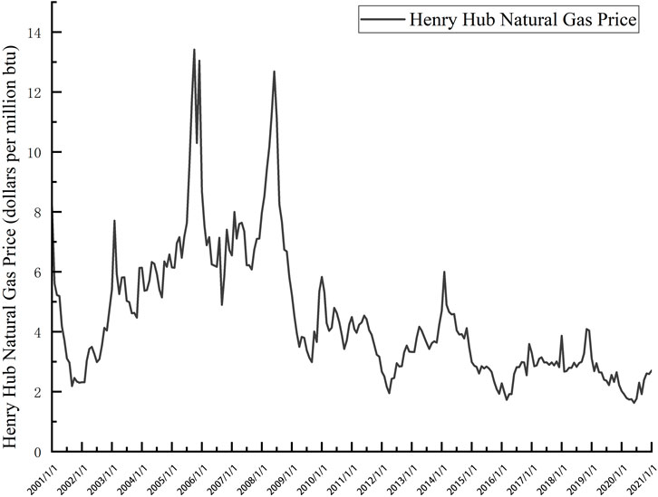
FIGURE 4. Henry Hub natural gas price time series.
In energy price forecasting, the raw data are mostly divided into training and test sets, and there is no uniformity in the division ratio (Lu H et al., 2021). In particular, we use a total of 202 (top 80%) monthly data from January 2001 to October 2017 as the training set and a total of 50 (bottom 20%) monthly data from November 2017 to December 2021 as the test set. The reason for selecting this time interval in this paper is that the natural gas price during this period has experienced two peak periods and three trough periods, with great volatility. Due to the forecasting process, there are always invariably unforeseen and uncontrollable “black swan” events that may occur. Due to this, we selected a period of time that avoids the uncontrollable factor of the Russian Ukrainian war during 2022. Since the collected coal price data are annual data and GDP data are quarterly data, this paper uses the EViews software to convert their frequencies to monthly data. Model training and testing are conducted with Spyder 5.4.3 (Python 3.9) software. The code in this study is implemented in Python. The experimental environment includes Windows 10 (64-bit), a Core (TM) i5-8250U CPU @1.80 GHz and 12.0 GB of RAM. For the plotting part, we used Origin 2022 and Visio software.
5.2 Evaluation criteria
In past research, multiple evaluation indicators were usually used to compare the developed model and other models for forecasting capacity. However, there is no specific standard that exists for model evaluation (Dong Y et al., 2020).
To better compare the prediction effect of models, we used five evaluation metrics to evaluate the prediction performance of models. They are the mean square error (MSE), mean absolute error (MAE), coefficient of determination (R2), root mean square error (RMSE), and mean absolute percentage error (MAPE). Among them, the lower values of MSE, MAE, RMSE, and MAPE signify the higher prediction accuracy of the model. Contrary to this, a greater R2 value indicates a more accurate fitting of the model. The mathematical formulas for each evaluation criteria are shown as follows:
where
5.3 Experimental results
5.3.1 Comparative analysis of forecast accuracy
To compare the performance of the different models clearly, a multi-level comparative analysis is performed in this paper. Figure 5 shows the fitting curves of different models. Figure 6 shows the histograms of the comparison of each model on five evaluation indicators. Table 6 demonstrates the detailed prediction accuracy of each model across the five evaluation indicators.
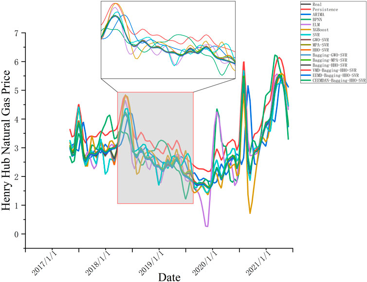
FIGURE 5. Comparison of predicted results of different models.
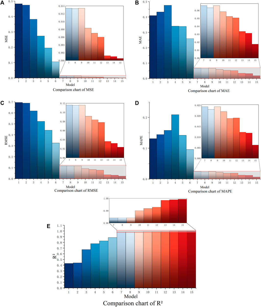
FIGURE 6. Comparison of predicted results of evaluation metrics. (A) Comparison of MSE, (B) comparison of MAE, (C) comparison of RMSE, (D) comparison of MAPE, and (E) comparison of R2.
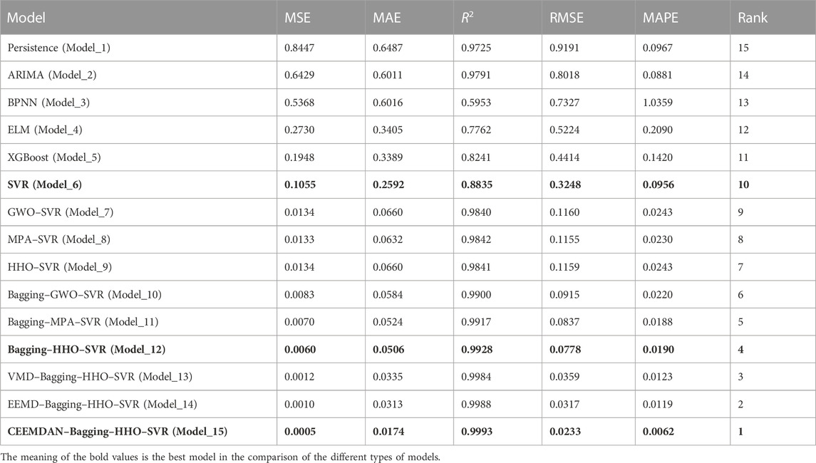
TABLE 6. Prediction accuracy comparison of different models.
The five evaluation indicators of the model are comprehensively compared. In the single model comparison, the values of MSE, RMSE, and R2 gradually decreased from the persistence model to the SVR model. However, the values of MAE improved from the persistence model to the BPNN model, and the values of MAPE increased from the persistence model to the ELM model. Generally, forecasting performance tends to improve. The economic model ARIMA performed only slightly better than the most basic persistence model in time series forecasting.
This may be because traditional economic models usually cannot fully capture the nonlinear characteristics of data and have certain limitations when facing long-term predictions and complex data. Moreover, ARIMA requires tedious parameter settings, which is a significant drawback compared to machine models. BPNN and ELM are both neural network models in machine learning. BPNN usually requires multiple iterations to adjust the weights and reduce the loss value. ELM can automatically adjust the hidden layer weights and bias, which trained only once without iterations. In this paper, ELM has better performance compared to BPNN. XGBoost has also been widely used in recent years in major research fields. It is suitable for medium and large sample data, and its performance in this study prediction is moderate. The regularization term added to it reduces the overfitting performance of the model. R2 is improved to 0.8241, but the rest of the evaluation metrics are general. This indicates that XGBoost may not be suitable for the dataset in this paper. The SVR model, a longstanding prediction model that has maintained stability with small-sample data over the decades, exhibits the same reliability in this paper. Compared with other single machine learning models, SVR showed high prediction accuracy. Therefore, the SVR model is selected for the subsequent study.
In the optimization model, three different optimization algorithms are combined with the SVR model for parameter finding. Compared to the single SVR model, the forecasting performance of all three optimization models has been improved. However, the performance of all three algorithms is almost the same. Therefore, we performed ensemble learning on all three algorithms.
In the ensemble model, the three optimization models GWO–SVR, MPA–SVR, and HHO–SVR are integrated and learned. In the comparison between the three ensemble models and the optimization model, all five evaluation indicators have improved. This is mainly a benefit by the Bagging algorithm reducing the variance of the model. The Bagging–HHO–SVR model performs most accurately among them, with better prediction accuracy for all five evaluation indicators compared to the others. This indicates that HHO combined with Bagging algorithm has better performance than the other two optimization algorithms. Therefore, we choose the Bagging–HHO–SVR model as the decomposed prediction model.
In the decomposition algorithms, we first used both EEMD and VMD decomposition methods for comparison. In order to compare with the new rolling decomposition method, we applied the old method to the EEMD and VMD decomposition which decomposes the whole time series. There is no significant difference in performance between the two algorithms, and both are stronger than the ensemble model, with EEMD performing slightly better than VMD. However, due to the problem of data leakage that this method may cause, we used the new rolling forecasting approach in the CEEMDAN decomposition algorithm. In this way, the dataset is decomposed many times and a large amount of future data is not included in the decomposition process. The prediction performance of this method is the best among all the algorithms. The CEEMDAN–Bagging–HHO–SVR model improves nearly 92% on MSE compared to the Bagging–HHO–SVR model.
Moreover, we conducted predictions and comparisons using different features before and after GRA screening as input variables for the CEEMDAN–Bagging–HHO–SVR model to demonstrate the effect of GRA on model performance. Table 7 shows the predicted results. From the table, we can see that in the prediction using GRA, the five evaluation indicators have significantly improved. Specifically, MSE values decreased from 0.0027 to 0.0005, MSE values decreased from 0.0468 to 0.0174, RMSE values decreased from 0.0528 to 0.0233, MAPE values decreased from 0.0159 to 0.0062, and R2 values increased from 0.9966 to 0.9993. This is mainly because we removed variables with low correlation through GRA, reduced the input dimension of the model, and thus improved prediction performance. As we can see, this method is indeed very effective, and this proves that the input variables we selected are reasonable and effective for the model.

TABLE 7. Comparison of prediction results before and after input variable screening.
The proposed hybrid model demonstrated excellent prediction results in Henry Hub’s empirical study of monthly natural gas prices. Furthermore, we also predicted NBP natural gas prices and Japan LNG prices to verify whether the model has the same excellent performance in other regions. Table 8 shows the prediction accuracy of different regions. The results show that the proposed model performed well in forecasting different regions. Therefore, the proposed model is not only applicable to Henry Hub natural gas prices but also has reference value for natural gas price research in other regions.
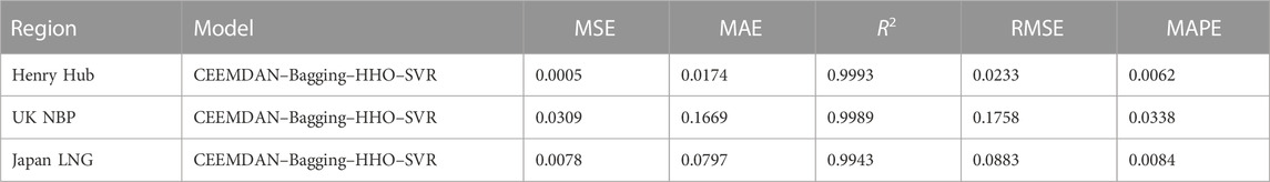
TABLE 8. Prediction results of the proposed model for different regions.
5.3.2 Characteristic importance analysis
Many current machine learning models can make accurate predictions, but they do not explain how they make them because complex problems often have black-box properties, although they can give high-accuracy results. It is difficult to explain the inner principles and which features have the most significant impact on prediction results. Therefore, we use the permutation importance method to analyze the feature importance of the Bagging–HHO–SVR model to assess how much each feature affects Henry Hub natural gas price prediction. The basic idea of the permutation importance method is to sequentially shuffle the sample order of each feature. Then, it evaluates the error size of the disordered feature compared to the normal prediction results. The larger the error, the more significant the effect of the feature on the prediction result. Figure 7 shows the result of permutation importance, which demonstrates the extent to which each feature influences Henry Hub natural gas prices.
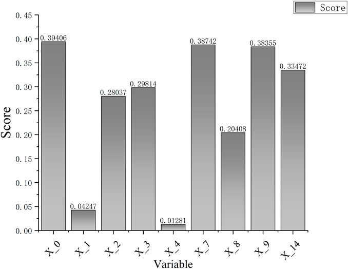
FIGURE 7. Histogram of feature importance.
According to the analysis results, historical natural gas prices, natural gas imports, and natural gas demand are among the top three factors. These factors are significant factors affecting Henry Hub’s natural gas price prediction. Among them, historical natural gas prices have the highest score. In univariate forecasts, historical natural gas prices are usually used as the only input variable. In multivariate forecasts, although many external influences are added as input variables, historical natural gas prices are still critical factors. It implies potential features such as long-term trends and seasonal fluctuations in natural gas prices, which are not present in external factors. Natural gas demand ranks second, with demand being a major component of the market’s supply and demand balance. When the demand for natural gas increases, the supply of natural gas is delayed and the market supply of natural gas may fall short of demand. Then, natural gas prices will increase. Conversely, when demand decreases, supply may exceed demand and the natural gas prices will decrease. Natural gas imports rank third. When there is a sudden increase in natural gas demand and the country cannot meet supply from its domestic natural gas production, it needs to import natural gas from abroad to bridge the demand gap. Consequently, natural gas imports alter natural gas prices by impacting supply and demand equilibrium, then influencing natural gas prices.
6 Conclusion and recommendations
Focusing on the nonlinearity and nonstationarity of natural gas prices caused by multiple influence factors and the limitations of single models, we proposed a CEEMDAN–Bagging–HHO–SVR hybrid model that considered various natural gas price influence factors and empirically analyzed the monthly natural gas price in Henry Hub in this paper. From the results of the empirical analysis over a 20-year period from January 2001 to December 2021, we can draw some conclusions:
(1) The CEEMDAN–Bagging–HHO–SVR model combines four algorithms: “decomposition algorithm,” “ensemble algorithm,” “optimization algorithm,” and “prediction model.” The addition of each algorithm further improves the forecasting performance of the model. The constructed model has extremely high prediction accuracy in forecasting natural gas prices in Henry Hub and also performs well in other regions. This indicates that the constructed model has universal applicability.
(2) In multivariate prediction, the choice of input variables is extremely important. We used GRA in this experiment to analyze the influence factors, which significantly improved the prediction accuracy of the model while reducing the subjectivity of input variable selection. Consequently, the input variables selected in this paper are very suitable for the forecasting of Henry Hub natural gas.
(3) Using a characteristic importance analysis, we conclude that historical natural gas prices, natural gas demand, and natural gas imports influence natural gas prices at Henry Hub greatly. This can provide some reference for relevant personnel.
Natural gas is emerging as a valuable, clean energy source, playing a vital economic and environmental role on a global scale as global natural gas trade expands. Energy market participants and policymakers require accurate natural gas price predictions. Energy companies can increase their competitiveness by formulating procurement strategies and pricing policies based on natural gas price predictions. For consumers, accurate natural gas price predictions can help them rationalize energy expenditures and reduce energy costs. Government agencies can also use natural gas price forecasts to optimize their energy policies and promote clean energy and sustainable development. As the most influential natural gas trading center in North America, the Henry Hub natural gas price fluctuations have a wide impact on the global energy market. The Henry Hub natural gas price is a major wind vane for international natural gas prices. Energy traders, investors, and energy users need to accurately forecast Henry Hub natural gas prices. Therefore, the proposed hybrid model is a potential analytical tool for investors interested in developing a strategic approach. Moreover, we put forward some recommendations based on the experimental results of this paper:
(1) For countries, the constantly changing international situation has a significant impact on the import and export of natural gas. The leaders of countries should always pay attention to the dynamics of major natural gas import and export countries. They should strengthen connections with these countries or sign strategic agreements to ensure the stability of their own natural gas import and export.
(2) For governments, it is necessary to strengthen its regulatory strategy on the natural gas market and strive to ensure the rationality of natural gas prices and the stability of the industrial chain. It is also important for the government to formulate energy diversification development strategies in the future in order to reduce its dependence on fossil fuels, for example, increasing policy incentives for the development of renewable energy sources such as solar and wind energy and developing various alternative energy sources to ensure the stability of the energy supply.
(3) For investors, they should adhere to long-term investment strategies and study the long-term development trends of historical prices. Investors should closely monitor government policy adjustments and international relations between countries to adjust their investment plans on time. In addition, investors can consider an investment portfolio that includes different types of energy to reduce the risk of natural gas price fluctuations on the investment.
There are still limitations to the experiment, even though the constructed model has extremely high accuracy in forecasting Henry Hub natural gas prices. There is inevitable subjectivity in the setting of some parameters due to the complexity of the experiment, such as the selection of multi-steps ahead and the selection of parameters for certain algorithms. To address this issue, more objective selection methods should be explored in future research.
Geopolitical risks are usually unforeseeable and have contingency. However, it cannot be denied that they have an unignored impact on natural gas price prediction, such as regional conflicts or policy changes in natural gas-producing countries that can lead to significant price fluctuations.
In addition, with the development of renewable energy technology and increased policy support, the competitiveness of renewable energy will affect the demand and price of natural gas. Although this paper considers some long-term factors affecting natural gas price changes, it cannot avoid the impact of policy factors and black swan events on prediction results. Thus, we did not consider some unexpected events such as geopolitical factors in this paper. Moreover, natural gas influence factors may change over time. Therefore, future research could try considering geopolitical factors and other influential factors with increasing importance to improve the applicability of models.
Data availability statement
The raw data supporting the conclusion of this article will be made available by the authors, without undue reservation.
Author contributions
YD: conceptualization and writing–review and editing. JZ: data curation, formal analysis, and writing–original draft. XW: methodology, supervision, and writing–review and editing.
Funding
The authors declare financial support was received for the research, authorship, and/or publication of this article. This research was funded by the National Natural Science Foundation of China (Grant No. 81973791).
Conflict of interest
The authors declare that the research was conducted in the absence of any commercial or financial relationships that could be construed as a potential conflict of interest.
Publisher’s note
All claims expressed in this article are solely those of the authors and do not necessarily represent those of their affiliated organizations, or those of the publisher, the editors, and the reviewers. Any product that may be evaluated in this article, or claim that may be made by its manufacturer, is not guaranteed or endorsed by the publisher.
Supplementary material
The Supplementary Material for this article can be found online at: https://www.frontiersin.org/articles/10.3389/fenrg.2023.1323073/full#supplementary-material
References
Açıkkar, M., and Altunkol, Y. (2023). A novel hybrid PSO- and GS-based hyperparameter optimization algorithm for support vector regression. Neural Comput. Appl. 35 (27), 19961–19977. doi:10.1007/s00521-023-08805-5
Alam, M. S., Murshed, M., Manigandan, P., Pachiyappan, D., and Abduvaxitovna, S. Z. (2023). Forecasting oil, coal, and natural gas prices in the pre-and post-COVID scenarios: contextual evidence from India using time series forecasting tools. Resour. Policy 81, 103342. doi:10.1016/j.resourpol.2023.103342
Arce, M. E., Saavedra, A., Miguez, J. L., and Granada, E. (2015). The use of grey-based methods in multi-criteria decision analysis for the evaluation of sustainable energy systems: a review. Renew. Sustain. Energy Rev. 47, 924–932. doi:10.1016/j.rser.2015.03.010
Arvanitidis, A. I., Bargiotas, D., Kontogiannis, D., Fevgas, A., and Alamaniotis, M. (2022). Optimized data-driven models for short-term electricity price forecasting based on signal decomposition and clustering techniques. Energies 15 (21), 7929. doi:10.3390/en15217929
Azadeh, A., Sheikhalishahi, M., and Shahmiri, S. (2012). A hybrid neuro-fuzzy simulation approach for improvement of natural gas price forecasting in industrial sectors with vague indicators. Int. J. Adv. Manuf. Technol. 62 (1-4), 15–33. doi:10.1007/s00170-011-3804-6
Bentéjac, C., Csörgő, A., and Martínez-Muñoz, G. (2020). A comparative analysis of gradient boosting algorithms. Artif. Intell. Rev. 54 (3), 1937–1967. doi:10.1007/s10462-020-09896-5
Cai, W., Wen, X., Li, C., Shao, J., and Xu, J. (2023). Predicting the energy consumption in buildings using the optimized support vector regression model. Energy 273, 127188. doi:10.1016/j.energy.2023.127188
Čeperić, E., Žiković, S., and Čeperić, V. (2017). Short-term forecasting of natural gas prices using machine learning and feature selection algorithms. Energy 140, 893–900. doi:10.1016/j.energy.2017.09.026
Chaudhuri, K., and Alkan, B. (2021). A hybrid extreme learning machine model with harris hawks optimisation algorithm: an optimised model for product demand forecasting applications. Appl. Intell. 52 (10), 11489–11505. doi:10.1007/s10489-022-03251-7
Cherkassky, V. (1997). The nature of statistical learning Theory∼∼. IEEE Trans. neural Netw., 8(6): 1564. doi:10.1109/TNN.1997.641482
Dong, Y., Li, J., Liu, Z., Niu, X., and Wang, J. (2022). Ensemble wind speed forecasting system based on optimal model adaptive selection strategy: case study in China. Sustain. ENERGY Technol. ASSESSMENTS 53 (B), 102535. doi:10.1016/j.seta.2022.102535
Dong, Y., Zhang, L., Liu, Z., and Wang, J. (2020). Integrated forecasting method for wind energy management: a case study in China. PROCESSES 8 (8), 35. doi:10.3390/pr8010035
Egbueri, J., and Agbasi, J. (2022). Data-driven soft computing modeling of groundwater quality parameters in southeast Nigeria: comparing the performances of different algorithms. Environ. Sci. Pollut. Res. 29 (25), 38346–38373. doi:10.1007/s11356-022-18520-8
Essa, F. A., Abd Elaziz, M., and Elsheikh, A. H. (2020). An enhanced productivity prediction model of active solar still using artificial neural network and Harris Hawks optimizer. Appl. Therm. Eng. 170, 115020. doi:10.1016/j.applthermaleng.2020.115020
Fang, T., Zheng, C., and Wang, D. (2023). Forecasting the crude oil prices with an EMD-ISBM-FNN model. Energy 263, 125407. doi:10.1016/j.energy.2022.125407
Faramarzi, A., Heidarinejad, M., Mirjalili, S., and Gandomi, A. H. (2020). Marine predators algorithm: a nature-inspired metaheuristic. Expert Syst. Appl. 152, 113377. doi:10.1016/j.eswa.2020.113377
Gao, R., Du, L., Duru, O., and Yuen, K. (2021). Time series forecasting based on echo state network and empirical wavelet transformation. Appl. Soft Comput. J. 102, 107111. doi:10.1016/j.asoc.2021.107111
Geng, J.-B., Ji, Q., and Fan, Y. (2016). The behaviour mechanism analysis of regional natural gas prices: a multi-scale perspective. Energy 101, 266–277. doi:10.1016/j.energy.2016.02.045
Heidari, A. A., Mirjalili, S., Faris, H., Aljarah, I., Mafarja, M., and Chen, H. (2019). Harris hawks optimization: algorithm and applications. Future Gener. Comput. Syst. 97, 849–872. doi:10.1016/j.future.2019.02.028
Hou, C., and Nguyen, B. H. (2018). Understanding the US natural gas market: a Markov switching VAR approach. Energy Econ. 75, 42–53. doi:10.1016/j.eneco.2018.08.004
Hou, H., Liu, C., Wang, Q., Wu, X. X., Tang, J. R., Shi, Y., et al. (2022). Review of load forecasting based on artificial intelligence methodologies, models, and challenges. Electr. Power Syst. Res. 210, 108067. doi:10.1016/j.epsr.2022.108067
Jiang, P., Liu, Z., Wang, J., and Zhang, L. (2022a). Decomposition-selection-ensemble prediction system for short-term wind speed forecasting. Electr. Power Syst. Res. 211, 108186. doi:10.1016/j.epsr.2022.108186
Jiang, P., Liu, Z., Zhang, L., and Wang, J. (2022b). Advanced traffic congestion early warning system based on traffic flow forecasting and extenics evaluation. Appl. Soft Comput. 118, 108544. doi:10.1016/j.asoc.2022.108544
Jianwei, E., Ye, J., He, L., and Jin, H. (2019). Energy price prediction based on independent component analysis and gated recurrent unit neural network. Energy 189, 116278. doi:10.1016/j.energy.2019.116278
Jung, S., Moon, J., Park, S., Rho, S., Baik, S. W., and Hwang, E. (2020). Bagging ensemble of multilayer perceptrons for missing electricity consumption data imputation. Sensors (Basel) 20 (6), 1772. doi:10.3390/s20061772
Kaur, J., Parmar, K., and Singh, S. (2023). Autoregressive models in environmental forecasting time series: a theoretical and application review. Environ. Sci. Pollut. Res. 30 (8), 19617–19641. doi:10.1007/s11356-023-25148-9
Li, H., Zhang, H.-M., Xie, Y.-T., and Wang, D. (2017). Analysis of factors influencing the Henry Hub natural gas price based on factor analysis. Petroleum Sci. 14 (4), 822–830. doi:10.1007/s12182-017-0192-z
Li, J., Wu, Q., Tian, Y., and Fan, L. (2021). Monthly Henry Hub natural gas spot prices forecasting using variational mode decomposition and deep belief network. Energy 227, 120478. doi:10.1016/j.energy.2021.120478
Li, Q., Li, D., Zhao, K., Wang, L., and Wang, K. (2022). State of health estimation of lithium-ion battery based on improved ant lion optimization and support vector regression. J. Energy Storage 50, 104215. doi:10.1016/j.est.2022.104215
Li, X., Sun, M., Gao, C., and He, H. (2019). The spillover effects between natural gas and crude oil markets: the correlation network analysis based on multi-scale approach. Phys. A Stat. Mech. its Appl. 524, 306–324. doi:10.1016/j.physa.2019.04.141
Liu, Z., Li, P., Wei, D., Wang, J., Zhang, L., and Niu, X. (2023). Forecasting system with sub-model selection strategy for photovoltaic power output forecasting. EARTH Sci. Inf. 16, 287–313. doi:10.1007/s12145-023-00938-4
Lu, H., Ma, X., Ma, M., and Zhu, S. (2021). Energy price prediction using data-driven models: a decade review. Comput. Sci. Rev. 39, 100356. doi:10.1016/j.cosrev.2020.100356
Lu, W., Qiu, T., Shi, W., and Sun, X. (2022). International gold price forecast based on CEEMDAN and support vector regression with grey wolf algorithm. Complexity 2022, 1–12. doi:10.1155/2022/1511479
Ma, M., and Wang, Z. (2019). Prediction of the energy consumption variation trend in South Africa based on ARIMA, NGM and NGM-ARIMA models. Energies 13 (1), 10. doi:10.3390/en13010010
Ma, X., Mei, X., Wu, W., Wu, X., and Zeng, B. (2019). A novel fractional time delayed grey model with Grey Wolf Optimizer and its applications in forecasting the natural gas and coal consumption in Chongqing China. Energy 178, 487–507. doi:10.1016/j.energy.2019.04.096
Meira, E., Cyrino Oliveira, F. L., and De Menezes, L. M. (2022). Forecasting natural gas consumption using Bagging and modified regularization techniques. Energy Econ. 106, 105760. doi:10.1016/j.eneco.2021.105760
Mienye, I., and Sun, Y. (2022). A survey of ensemble learning: concepts, algorithms, applications, and prospects. IEEE ACCESS 10, 99129–99149. doi:10.1109/ACCESS.2022.3207287
Mirjalili, S., Mirjalili, S. M., and Lewis, A. (2014). Grey wolf optimizer. Adv. Eng. Softw. 69, 46–61. doi:10.1016/j.advengsoft.2013.12.007
Mohammed, A., and Kora, R. (2023). A comprehensive review on ensemble deep learning: opportunities and challenges. J. King Saud Univ. – Comput. Inf. Sci. 35 (2), 757–774. doi:10.1016/j.jksuci.2023.01.014
Mohammed, S., Zubaidi, S., Al-Ansari, N., Ridha, H., and Al-Bdairi, N. (2022). Hybrid technique to improve the river water level forecasting using artificial neural network-based marine predators algorithm. Adv. Civ. Eng. 2022, 1–14. doi:10.1155/2022/6955271
Ngo, N., Truong, T., Truong, N., Pham, A., Huynh, N., Pham, T., et al. (2022). Proposing a hybrid metaheuristic optimization algorithm and machine learning model for energy use forecast in non residential buildings. Sci. Rep. 12 (1), 1065. doi:10.1038/s41598-022-04923-7
Pannakkong, W., Harncharnchai, T., and Buddhakulsomsiri, J. (2022). Forecasting daily electricity consumption in Thailand using regression, artificial neural network, support vector machine, and hybrid models. Energies 15 (9), 3105. doi:10.3390/en15093105
Pei, Y., Huang, C., Shen, Y., and Ma, Y. (2022). An ensemble model with adaptive variational mode decomposition and multivariate temporal graph neural network for PM2.5 concentration forecasting. Sustainability 14 (20), 13191. doi:10.3390/su142013191
Qian, Z., Pei, Y., Zareipour, H., and Chen, N. (2019). A review and discussion of decomposition-based hybrid models for wind energy forecasting applications. Appl. Energy 235, 939–953. doi:10.1016/j.apenergy.2018.10.080
Rabbi, M. F., Popp, J., Mate, D., and Kovacs, S. (2022). Energy security and energy transition to achieve carbon neutrality. Energies 15 (21), 8126. doi:10.3390/en15218126
Salehnia, N., Falahi, M. A., Seifi, A., and Mahdavi Adeli, M. H. (2013). Forecasting natural gas spot prices with nonlinear modeling using Gamma test analysis. J. Nat. Gas Sci. Eng. 14, 238–249. doi:10.1016/j.jngse.2013.07.002
Sharma, M., and Shekhawat, H. (2022). Portfolio optimization and return prediction by integrating modified deep belief network and recurrent neural network. Knowledge-Based Syst. 250, 109024. doi:10.1016/j.knosys.2022.109024
Son, H.-G., Kim, Y., and Kim, S. (2020). Time series clustering of electricity demand for industrial areas on smart grid. Energies 13 (9), 2377. doi:10.3390/en13092377
Stajic, L., Dordevic, B., Ilic, S., and Brkic, D. (2021). The volatility of natural gas prices - structural shocks and influencing factors. Rev. Int. De. Metodos Numer. Para. Calc. Y Diseno En. Ing. 37 (4), 12. doi:10.23967/j.rimni.2021.12.002
Su, M., Zhang, Z., Zhu, Y., Zha, D., and Wen, W. (2019). Data driven natural gas spot price prediction models using machine learning methods. Energies 12 (9), 1680. doi:10.3390/en12091680
Su, X., He, X., Zhang, G., Chen, Y., and Li, K. (2022). Research on SVR water quality prediction model based on improved sparrow search algorithm. Comput. Intell. Neurosci. 2022, 1–23. doi:10.1155/2022/7327072
Sun, Y., Dong, J., Liu, Z., and Wang, J. (2023). Combined forecasting tool for renewable energy management in sustainable supply chains. Comput. Industrial Eng. 179, 109237. doi:10.1016/j.cie.2023.109237
Torres, M. ı. E., Colominas, M. A., Schlotthauer, G. N., and Flandrin, P. (2011). “A complete ensemble empirical mode decomposition with adaptive noise,” in 2011 IEEE International Conference on Acoustics, Speech and Signal Processing (ICASSP), Prague, Czech Republic, May, 2011.
Wang, J., Cao, J., Yuan, S., and Cheng, M. (2021). Short-term forecasting of natural gas prices by using a novel hybrid method based on a combination of the CEEMDAN-SE-and the PSO-ALS-optimized GRU network. Energy 233, 121082. doi:10.1016/j.energy.2021.121082
Wang, J., Lei, C., and Guo, M. (2020b). Daily natural gas price forecasting by a weighted hybrid data-driven model. J. Petroleum Sci. Eng. 192, 107240. doi:10.1016/j.petrol.2020.107240
Wang, J., Zhang, L., Liu, Z., and Niu, X. (2022). A novel decomposition-ensemble forecasting system for dynamic dispatching of smart grid with sub-model selection and intelligent optimization. Expert Syst. Appl. 201, 117201. doi:10.1016/j.eswa.2022.117201
Wang, Y., Wang, L., Chang, Q., and Yang, C. (2020a). Effects of direct input–output connections on multilayer perceptron neural networks for time series prediction. Soft Comput. 24 (7), 4729–4738. doi:10.1007/s00500-019-04480-8
Wang, Y., Wang, Z., Wang, X., and Kang, X. (2023). Multi-step-ahead and interval carbon price forecasting using transformer-based hybrid model. Environ. Sci. Pollut. Res. 30 (42), 95692–95719. doi:10.1007/S11356-023-29196-Z
Wu, Z., and Huang, N. E. (2009). Ensemble empirical mode decomposition: a noise-assisted data analysis method. Adv. Adapt. Data Analysis 1 (01), 1–41. doi:10.1142/s1793536909000047
Yahşi, M., Çanakoğlu, E., and Ağralı, S. (2019). Carbon price forecasting models based on big data analytics. Carbon Manag. 10 (2), 175–187. doi:10.1080/17583004.2019.1568138
Youssef, M., Mokni, K., and Ajmi, A. N. (2021). Dynamic connectedness between stock markets in the presence of the COVID-19 pandemic: does economic policy uncertainty matter? Financ. Innov. 7 (1), 13. doi:10.1186/s40854-021-00227-3
Yu, L., and Yang, Z. (2022). Evaluation and analysis of electric power in China based on the ARMA model. Math. Problems Eng. 2022, 1–6. doi:10.1155/2022/5017751
Yu, Y., Wang, J., Liu, Z., and Zhao, W. (2021). A combined forecasting strategy for the improvement of operational efficiency in wind farm. J. Renew. Sustain. Energy 13 (6). doi:10.1063/5.0065937
Zhan, L., Tang, Z., and Frausto-Solis, J. (2022). Natural gas price forecasting by a new hybrid model combining quadratic decomposition technology and LSTM model. Math. Problems Eng. 2022, 1–13. doi:10.1155/2022/5488053
Zhang, L., Wang, J., and Liu, Z. (2022). Power grid operation optimization and forecasting using a combined forecasting system. J. Forecast. 42 (1), 124–153. doi:10.1002/for.2888
Zhang, T., Tang, Z., Wu, J., Du, X., and Chen, K. (2021b). Multi-step-ahead crude oil price forecasting based on two-layer decomposition technique and extreme learning machine optimized by the particle swarm optimization algorithm. Energy 229, 120797. doi:10.1016/j.energy.2021.120797
Zhang, W., and Hamori, S. (2020). Do machine learning techniques and dynamic methods help forecast US natural gas crises? Energies 13 (9), 2371. doi:10.3390/en13092371
Zhang, Y., Peng, Y., Qu, X., Shi, J., and Erdem, E. (2021a). A finite mixture GARCH approach with EM algorithm for energy forecasting applications. Energies 14 (9), 2352. doi:10.3390/en14092352
Zheng, Y., Luo, J., Chen, J., Chen, Z., and Shang, P. (2023). Natural gas spot price prediction research under the background of Russia-Ukraine conflict - based on FS-GA-SVR hybrid model. J. Environ. Manage 344, 118446. doi:10.1016/j.jenvman.2023.118446
Zhu, H., Chong, L., Wu, W., and Xie, W. (2023). A novel conformable fractional nonlinear grey multivariable prediction model with marine predator algorithm for time series prediction. Comput. Industrial Eng. 180, 109278. doi:10.1016/j.cie.2023.109278
Keywords: natural gas price forecasting, Henry Hub, SVR, CEEMDAN decomposition, Bagging, HHO algorithm
Citation: Duan Y, Zhang J and Wang X (2023) Henry Hub monthly natural gas price forecasting using CEEMDAN–Bagging–HHO–SVR. Front. Energy Res. 11:1323073. doi: 10.3389/fenrg.2023.1323073
Received: 17 October 2023; Accepted: 20 November 2023;
Published: 14 December 2023.
Edited by:
Furkan Ahmad, Hamad Bin Khalifa University, QatarReviewed by:
Ruobin Gao, Nanyang Technological University, SingaporeLifang Zhang, Dongbei University of Finance and Economics, China
Copyright © 2023 Duan, Zhang and Wang. This is an open-access article distributed under the terms of the Creative Commons Attribution License (CC BY). The use, distribution or reproduction in other forums is permitted, provided the original author(s) and the copyright owner(s) are credited and that the original publication in this journal is cited, in accordance with accepted academic practice. No use, distribution or reproduction is permitted which does not comply with these terms.
*Correspondence: Yonghui Duan, MzI3NDc3MzAwQHFxLmNvbQ==