A multi-task transient stability assessment method adapted to topology changes using multi-graph sample and aggregate-attention network

Transient stability assessment (TSA) plays a pivotal role in guiding power grid risk control strategies. However, it faces challenges when dealing with complex multi-graph inputs generated by pre-fault, fault occurrence, and post-fault states. Meanwhile, most previous research studies neglected the assessment of the transient stability level. To address this, we propose a multi-task transient stability assessment (MTTSA) approach. In MTTSA, we introduce a multi-graph sample and aggregate-attention network (GraphSAGE-A) designed to capture stability features even amidst topology changes. A multi-head attention mechanism and local normalization method are adopted for a better extraction of the global and contextual information. Additionally, we introduce a quantified transient stability risk index considering the transient stability boundary and incorporate a multi-task dense structure to enhance MTTSA’s performance. Empirical tests, under changing operating conditions, conducted on the IEEE 39-bus system showcase a significant performance improvement with the proposed MTTSA method.

1 Introduction

With the increasing penetration of renewable energy and widespread utilization of power electronic devices, the modern power system becomes less resistant to disturbances and, thus, requires more reliable and effective transient stability assessment (TSA) methods. On one hand, the accuracy and speed of traditional analysis methods have been challenged. On the other hand, most previous studies concentrated on the binary stability category, which rarely concerned a quantified stability risk assessment under the influence of TSB. In such contexts, it is essential to adopt a multi-task transient stability assessment (MTTSA) method in order to predict the risk levels and activate emergency control on time.

The practical implementation of TSA is facilitated by the rapid proliferation of phasor measurement units (PMUs) (Gurusinghe and Rajapakse, 2016) and the development of feature extraction technology in power grids. PMUs provide real-time load monitoring data, and modern artificial intelligence algorithms can effectively extract features of large amounts of data.

As is shown in Table 1, traditional TSA is previously combined with the direct method of transient stability analysis and the time-domain simulation technique (Maria et al., 1990). To improve the accuracy of prediction, researchers proposed a fully time-domain simulation (TDS)-based method (Diao et al., 2017), which solves high-dimensional nonlinear differential-algebraic equations (DAEs) of the power system using numerical integration algorithms. However, the results of this numerical differentiation greatly depend on the parameters of power grid models, such as synchronous generators, loads, transmission lines, and emergency control devices. In addition, the increasing time costs brought by the growing scale of the power system limits the speed of the TDS-based method (Senyuk et al., 2023).

TABLE 1

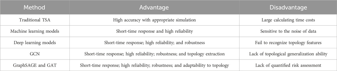
TABLE 1. Comparison of previous studies.

The goal of online TSA is realized due to the development of machine learning (ML) and deep learning methods. Liu et al. (2020) and Liu et al. (2021) developed the transient stability margin with the concept of critical clearing time (CCT), which is tested to easily change through multiple time-domain simulations. The qualitative methods based on the analysis of the kinetic energy of a generator rotor before, during, and after a contingency gradually develop stability criteria and form the trajectory-based transient stability index (TSI) (Glavic et al., 2007; Xu et al., 2015). The deployment of high-precision PMUs (Gurusinghe and Rajapakse, 2016) has led to an increase in the rate of power system parameter sampling, which, in turn, supports the utilization of large data in ML-based methods. The model-free ML methods, such as artificial neural network (ANN) (Siddiqui et al., 2018), support vector machine (SVM) (Gomez et al., 2011), and random forest (Mukherjee and De, 2020), can solve the problem of TSA. ANNs with a parallel structure were first applied to TSA (Siddiqui et al., 2018). Nonetheless, ANN-based TSA algorithms have not been widely adopted due to computational limitations. SVMs were used to process the binary classification task of TSA with short-time response and high reliability, but it is sensitive to the inevitable noise of input data. There are decision tree-based methods including fuzzy decision tree (Kamwa et al., 2012) and random forest (Mukherjee and De, 2020) with drawbacks of the proneness to re-training. Overall, the mentioned TSA algorithms are willing to overfit restrictions by generalization ability.

Different from traditional ML methods, deep learning models are capable of handling significantly larger-scale data by automatically generating features from raw input. Yu et al. (2018) developed a TSA system based on the long short-term memory network (LSTM) to capture the long-term dependencies along the time steps of time series. Furthermore, an LSTM-based gated recurrent unit is added to a two-stage TSA method for the analysis of uncertain samples after the first stage (Zhan et al., 2022). Convolutional neural network (CNN) is also widely used in many outstanding TSA models (Gupta et al., 2019; Shi et al., 2020). The time series sampled by PMUs are mapped into heatmap representation (Kamwa et al., 2012) or processed as a multi-channel matrix (Shi et al., 2020) to leverage the strengths of CNN in learning representations from images. Additionally, the gated recurrent unit model is developed to process the time-adaptive TSA (Chen and Wang, 2021). Moreover, an attention mechanism is introduced and combined with bidirectional (Bi)-LSTM to extract more robust features (Mahato et al., 2021). Nevertheless, a power grid inherently exhibits a structured graph representation, where buses are modeled as nodes and transmission lines are modeled as edges (Ishizaki et al., 2018). CNN, LSTM, or Bi-LSTM attention mechanisms failed to effectively recognize the system’s topological features, which has an impact on TSA tasks.

Fortunately, the introduction of graph neural networks (GNNs) provides a promising approach for addressing the aforementioned issues. Although bus-modeled nodes possess numerous temporal features, the effectiveness of combining the TSA method based on random walk-based GNN is not satisfactory. The GNN models, including graph convolutional network (GCN) (Huang et al., 2020), graph sample and aggregate network (GraphSAGE) (Lin et al., 2022), and graph attention network (GAT) (Huang et al., 2021), effectively handled both the temporal and system topological features of nodes and are widely utilized in TSA tasks. Huang et al. (2020) proposed the online TSA comprising GCN, which explicitly integrates the bus (node) states with the topological characteristics. The GCN model is also capable of power grid fault location prediction and load shedding decision (Kim et al., 2019; Chen et al., 2020). As variants of GCN, GraphSAGE and GAT models enable the automatic generation of small-scale topological changes from raw samples.

The trajectory-based TSI observed in power systems is widely applied for the qualitative assessment of transient stability, but the fixed TSB affects the overall generalization ability of TSA methods for diverse samples (Yan et al., 2021). Zheng et al. (2017) transformed the TSA problem into a relationship between state space using time series approximation and the region of attraction, while Du and Hu (2021) and Li et al. (2021) quantified the transient stability risk of uncertain samples using the TSB associated with sample orientation in a two-stage LSTM-based approach. A trajectory-based piece-wise stability index (PSI) was developed by Huang et al. (2021) to describe the transient stability level instead of CCT.

In our study, we design a multi-graph sample and aggregate-attention network (GraphSAGE-A) for MTTSA feature aggregation. A multi-head attention mechanism is utilized to replace the global information aggregation from the neighbors, while the extraction for contextual features is addressed by the local normalization for edge weights. A TSI-based transient stability prediction task (TSP) and a quantified transient stability risk prediction task (QRP) considering the uncertain samples of TSP work in parallel and share the features abstracted by GraphSAGE-A. A transient stability risk index (RI) is developed to instruct the subsequent risk control. The main contributions of this paper are summarized as follows:

1) A multi-graph GraphSAGE-A model requires the system dynamics before, during, and after a fault ($t_{0^{-}}$, $t_{0^{+}}$, and $t_{c^{+}}$) as input and realizes TSA with good precision even under topological changes.

2) A multi-head attention mechanism is adopted to extract the global and contextual information better, while the local normalization method for edge weights is proposed to improve the generalization ability for the subgraph.

3) A multi-task method concurrently considers the transient stability qualitative and quantitative analyses. An RI, considering the variability across different samples, is proposed to quantify the extent of the deviation from TSB.

The rest of this paper is organized as follows. Section 2 proposes the topology adaptive MTTSA method, while Section 3 presents the designs of GraphSAGE-A in detail. Experiments are conducted on the IEEE 39-bus system and discussed in Section 4. Finally, the conclusion is provided in Section 5.

2 Topology adaptive multi-task transient stability assessment method

2.1 MTTSA problem modeling

From a mathematical perspective, the power system TSA can be modeled by high-dimensional nonlinear DAEs with initial conditions at three snapshots as follows:

$\left\{\begin{array}{c}\begin{array}{c}\frac{dx}{dt}=f\left(x,y\right)\\ 0=g_G\left(x,y\right)\\ {\left.\left(x,y\right)\right|}_{t_{0-}}=\left(x_0,y_0\right)\end{array}\\ {\left.G\right|}_{t_{0-}}=G_{0-}\\ {\left.G\right|}_{t_{0+}}=G_{0+}\\ {\left.G\right|}_{t_{c+}}=G_{c+}\end{array}\right.,(1)$

where vector $x$ represents the state variables including dynamic generator rotor angles and bus voltages, while vector $y$ denotes the algebraic variables (e.g., the static impedance of transmission lines). ${\left.G\right|}_{t_j}$, $j=0-,0+,c+$ represents the parameterized network topologies of the graph type (Ishizaki et al., 2018) at the $j^{th}$ sampling shot before, during, and after a fault.

The mentioned data-driven TSA methods, using ML (Kamwa et al., 2012; Siddiqui et al., 2018) or deep learning models (Ishizaki et al., 2018; Yu et al., 2018), calculate the full-time series features of the period $\left\{{\left.\left(x,y\right)\right|}_t\right\},t\in t_{0-}\cup \left[t_{0+},t_{c+}+k\Delta t\right]$. Here, $\Delta t$ stands for a time step with $k>0$. The pre-fault one, which evaluates the transient stability for a pre-defined disturbance setting, relies on numerical analysis to solve DAEs. In contrast, the post-fault one focuses on evaluating the stability trends during the occurrence of a contingency, which leads to increased demands for dynamics from PMUs after the fault. Both pre- and post-fault methods explored the correlations among the state variables, particularly the relationship between generator rotor angles and other state variables. Nevertheless, they failed to provide fast predictions because of the time-consuming TDS or a significant number of PMU sampling.

Three snapshots ($t_{0^{-}}$, $t_{0^{+}}$, and $t_{c^{+}}$) utilized instead of the period $\left\{{\left.\left(\mathit{x},y\right)\right|}_t\right\},t\in t_{0-}\cup \left[t_{0+},t_{c+}+k\Delta t\right]$ realized online TSA by avoiding the vast majority of TDS or PMU sampling. However, we need to adopt the MTTSA method with a better ability for feature extraction, especially the topological structure.

2.2 Design of the MTTSA method

Regarding the significant requirement for topology representation learning, GraphSAGE-A becomes the critical point of the proposed MTTSA method, as shown in Figure 1. The aggregate-attention layers in the multi-graph node embedding module generate features for TSP and QRP modules. Considering the ensemble learning, we develop two predictor tasks, where TSP refers to the binary classification problem and QRP constructs the regression model. Both TSP and QRP belong to the full-connected network. Then, the MTTSA method is divided into the joint-training stage and the applying stage. In the joint-training stage, the sample loader structure allows mini-batch training for GraphSAGE-A, while TSP and QRP share the output from the multi-graph node-embedding module.

FIGURE 1

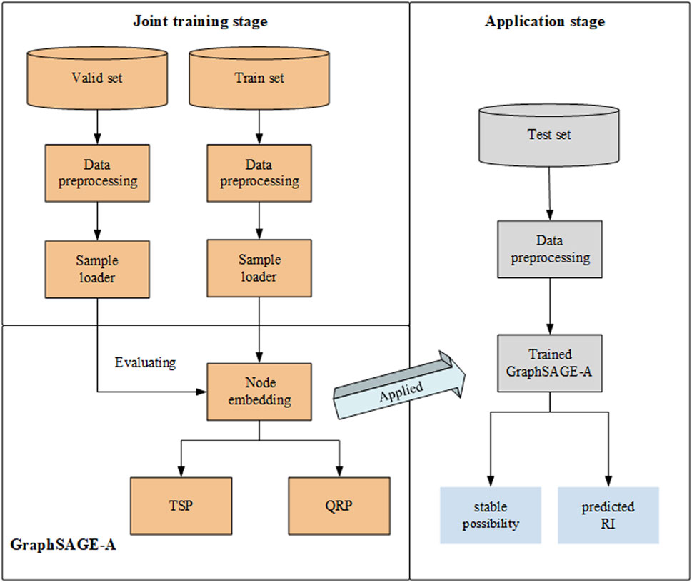
FIGURE 1. MTTSA method.

Meanwhile, the design with the labels of various tasks guarantees stability concerning coarse- and fine-grained embedding captured. As a result, richer inter-task information leads to the better performance of both TSP and QRP. During the online applying stage, state variables from TDS or PMU sampling are input into the trained GraphSAGE-A to generate the stable possibility $\widehat{p}$ from TSP and the predicted RI $\widehat{\nu }$ from QRP.

3 Multi-graph sample and aggregate-attention network

3.1 Model input and data preprocessing

Considering the dynamic embedding from TDS or PMU sampling, the amplitude and phase angle of voltage and the active and reactive power of both generators and loads had a total of four dimensional features for the $\mathrm{i}-\text{th}$ bus at the $\mathrm{j}-\text{th}$ snapshot. The raw input of the $\mathrm{K}-\text{th}$ sample can be described as the following matrix ${\mathrm{X}}_{\mathrm{K}}\in {\mathrm{R}}^{\mathrm{m}\times 4\mathrm{n}}$:

${\mathrm{X}}_{\mathrm{K}}=\left(\begin{array}{ccc}{\mathrm{U}}_{11}{,\mathrm{\theta }}_{11}{,\mathrm{P}}_{11},{\mathrm{Q}}_{11},& \cdots ,{\mathrm{U}}_{1\mathrm{i}},{\mathrm{\theta }}_{1\mathrm{i}},{\mathrm{P}}_{1\mathrm{i}},{\mathrm{Q}}_{1\mathrm{i}},& \cdots ,{\mathrm{U}}_{1\mathrm{n}},{\mathrm{\theta }}_{1\mathrm{n}},{\mathrm{P}}_{1\mathrm{n}},{\mathrm{Q}}_{1\mathrm{n}}\\ ⋮& \ddots & ⋮\\ {\mathrm{U}}_{\mathrm{j}1},{\mathrm{\theta }}_{\mathrm{j}1},{\mathrm{P}}_{\mathrm{j}1},{\mathrm{Q}}_{\mathrm{j}1},& \cdots ,{\mathrm{U}}_{\text{ji}},{\mathrm{\theta }}_{\text{ji}},{\mathrm{P}}_{\text{ji}},{\mathrm{Q}}_{\text{ji}},& \cdots {,\mathrm{U}}_{\text{jn}},{\mathrm{\theta }}_{\text{jn}},{\mathrm{P}}_{\text{jn}},{\mathrm{Q}}_{\text{jn}}\\ ⋮& \ddots & ⋮\\ {\mathrm{U}}_{\mathrm{m}1},{\mathrm{\theta }}_{\mathrm{m}1},{\mathrm{P}}_{\mathrm{m}1},{\mathrm{Q}}_{\mathrm{m}1},& \cdots ,{\mathrm{U}}_{\text{mi}},{\mathrm{\theta }}_{\text{mi}},{\mathrm{P}}_{\text{mi}},{\mathrm{Q}}_{\text{mi}},& \cdots {,\mathrm{U}}_{\text{mn}},{\mathrm{\theta }}_{\text{mn}},{\mathrm{P}}_{\text{mn}},{\mathrm{Q}}_{\text{mn}}\end{array}\right),(2)$

where ${\mathrm{U}}_{\text{ji}}$, ${\mathrm{\theta }}_{\text{ji}}$, ${\mathrm{P}}_{\text{ji}}$, and ${\mathrm{Q}}_{\text{ji}}$ represent the voltage amplitude, voltage phase angle, active power, and reactive power of the $\mathrm{i}-\text{th}$ node at the $\mathrm{j}-\text{th}$ shot, respectively. Following the z-score normalization, the data are performed as follows:

${\mathrm{X}}^{*}=\frac{\mathrm{X}-\mathrm{\mu }}{\mathrm{\sigma }}.(3)$

${\mathrm{X}}^{*}$ is the normalized value of $\mathrm{X}$, and $\mathrm{\mu }$ and $\mathrm{\sigma }$ are the mean and standard deviation of the features, respectively.

The number of input graph nodes refers to the total buses of the power grid, while the information of edges refers to the transmission lines. The multi-graph representing the single sample is defined as follows:

${\mathrm{G}}_{\text{Kj}}=\left({\mathrm{V}}_{\text{Kj}},{\mathrm{A}}_{\text{Kj}}\right).(4)$

${\mathrm{G}}_{\text{Kj}}$ represents the graph of the $\mathrm{K}-\text{th}$ sample at the $\mathrm{j}-\text{th}$ snapshot, while ${\mathrm{V}}_{\text{kj}}$ represents the $\mathrm{j}-\text{th}$ row of the normalized ${\mathrm{X}}_{\mathrm{K}}$. ${\mathrm{A}}_{\text{Kj}}$ is the adjacency matrix. The formula is

${\mathrm{A}}_{\text{Kj}}\left[\mathrm{u}\right]\left[\mathrm{v}\right]=\left\{\begin{array}{cc}0& \left(\mathrm{u},\mathrm{V}\right)\notin {\mathrm{E}}_{\text{kj}}\\ \left|{\mathrm{Z}}_{\mathrm{m}\left(\mathrm{v},\mathrm{u}\right)}\right|& \left(\mathrm{V},\mathrm{V}\right)\in {\mathrm{E}}_{\text{kj}}\\ 1& \mathrm{u}=\mathrm{v}\end{array}\right.,(5)$

where ${\mathrm{A}}_{\text{Kj}}\left[\mathrm{u}\right]\left[\mathrm{v}\right]$ are the element of the matrix ${\mathrm{A}}_{\text{Kj}}$ following the location $\left(\mathrm{u},\mathrm{v}\right)$, while $\mathrm{v}$ and $\mathrm{u}$ are any two node indices of the graph ${\mathrm{G}}_{\text{Kj}}$. ${\mathrm{E}}_{\text{Kj}}\left[\mathrm{u}\right]\left[\mathrm{v}\right]$ and $\left|{\mathrm{Z}}_{\text{Kj}\left(\mathrm{v},\mathrm{u}\right)}\right|$ denote the existence and static impedance of a transmission line from the $\mathrm{v}-\text{th}$ bus to the $\mathrm{u}-\text{th}$ bus at the $\mathrm{j}-\text{th}$ snapshot of the $\mathrm{K}-\text{th}$ sample, respectively.

3.2 GraphSAGE

For each node targeted of the given ${\mathrm{G}}_{\text{Kj}}$, the GraphSAGE model samples the neighbors and aggregates their features to the neighbors’ vector ${\mathrm{h}}_{\mathrm{N}\left(\mathrm{v}\right)}^{\mathrm{k}}$ depending on the representations of the previous stage:

${\mathrm{h}}_{\mathrm{N}\left(\mathrm{v}\right)}^{\mathrm{k}}={\text{AGG}}_{\mathrm{k}}\left(\text{WeightNorm}\left({\mathrm{A}}_{\text{Kj}}\left[\mathrm{u}\right]\left[\mathrm{v}\right]\right)\ast {\mathrm{h}}_{\mathrm{u}}^{\mathrm{k}-1},\forall \mathrm{u}\in \mathrm{N}\left(\mathrm{v}\right)\right),(6)$

where $\mathrm{k}$ refers to the $\mathrm{k}-\text{th}$ stage and $\mathrm{N}\left(\mathrm{v}\right)$ denotes the neighbor indices of the target node index $\mathrm{v}$. The 1-hop neighbors indices, whose corresponding element with $\mathrm{v}$ in the adjacency matrix is not 0 or 1, are usually utilized according to the size of the graph. ${\text{AGG}}_{\mathrm{k}}$ is defined as the method at the $\mathrm{k}-\text{th}$ stage to process the representations, including mean, pooling and LSTM. In addition, the initial representations of node indices are the normalized node features.

${\mathrm{h}}_{\mathrm{v}}^0=\left({\mathrm{U}}_{\text{jv}}^{*},{\mathrm{\theta }}_{\text{jv}}^{*},{\mathrm{P}}_{\text{jv}}^{*},{\mathrm{Q}}_{\text{jv}}^{*}\right)\in {\mathrm{V}}_{\text{Kj}}.(7)$

${\mathrm{U}}_{\text{jv}}^{*}$, ${\mathrm{\theta }}_{\text{jv}}^{*}$, ${\mathrm{P}}_{\text{jv}}^{*}$, and ${\mathrm{Q}}_{\text{jv}}^{*}$ are the elements of node features ${\mathrm{V}}_{\text{Kj}}$. Here, we adopt the local normalization of the adjacency matrix to meet the requirements of local aggregation as needed by the GraphSAGE algorithm. The method is

$\text{WeightNorm}\left({\mathrm{A}}_{\text{Kj}}\left[\mathrm{u}\right]\left[\mathrm{v}\right]\right)=\frac{{\mathrm{A}}_{\text{Kj}}\left[\mathrm{u}\right]\left[\mathrm{v}\right]}{{\displaystyle {\sum }_{\mathrm{h}\in \mathrm{N}\left(\mathrm{v}\right)}}{\mathrm{A}}_{\text{Kj}}\left[\mathrm{h}\right]\left[\mathrm{v}\right]},\forall \mathrm{u}\in \mathrm{N}\left(\mathrm{v}\right),(8)$

where $\text{WeightNorm}\left({\mathrm{A}}_{\text{Kj}}\left[\mathrm{u}\right]\left[\mathrm{v}\right]\right)$ refers to the result of local normalization for the edge from the $\mathrm{u}-\text{th}$ node to the $\mathrm{v}-\text{th}$ node and ${\mathrm{A}}_{\text{Kj}}\left[\mathrm{u}\right]\left[\mathrm{v}\right]$ stands for the element of ${\mathrm{A}}_{\text{Kj}}$ according to the location $\left(\mathrm{u},\mathrm{v}\right)$.

Then, the node index $\mathrm{v}$ tends to form its own vector ${\mathrm{h}}_{\mathrm{v}}^{\mathrm{k}}$ at the $\mathrm{k}-\text{th}$ stage for the next step such that

${\mathrm{h}}_{\mathrm{v}}^{\mathrm{k}}=\mathrm{\sigma }\left({\mathrm{W}}^{\mathrm{k}}\bullet \text{CONCAT}\left({\mathrm{h}}_{\mathrm{v}}^{\mathrm{k}-1},{\mathrm{h}}_{\mathrm{N}\left(\mathrm{v}\right)}^{\mathrm{k}}\right)\right),(9)$

where $W^k$ is the weight matrix for the training of the $k-\text{th}$ stage. $\sigma$ is usually the ReLU function for activation, and $CONCAT$ denotes the concatenating method for the input given.

3.3 Graph attention

The association degree differs between different nodes (Ding et al., 2022). It means the differences between global and contextual information cannot be performed in the weight set by the aggregation functions of the GraphSAGE model. A graph attention mechanism can compute the relationship between any two nodes regardless of their adjacency to extract the global view in the graph. Hence, the graph attention mechanism is used as the aggregation method to weigh the significance of the nodes among the neighbors. Furthermore, a multi-head graph attention mechanism allows multiple graph attention blocks to work in parallel to aggregate more contextual information at the same time.

First, a multi-head function is defined as follows:

$\text{Multihead}{\left(\mathrm{m}\right)}_{\left(\mathrm{v},\mathrm{u}\right)}^{\mathrm{k}}=\left(\begin{array}{c}\text{CONCAT}\left(\mathrm{W}{\mathrm{h}}_{\mathrm{v}}^{\mathrm{k}-1,1},\mathrm{W}{\mathrm{h}}_{\mathrm{u}}^{\mathrm{k}-1,1},\right)\\ ...\\ \text{CONCAT}\left(\mathrm{W}{\mathrm{h}}_{\mathrm{v}}^{\mathrm{k}-1,\mathrm{m}},\mathrm{W}{\mathrm{h}}_{\mathrm{u}}^{\mathrm{k}-1,\mathrm{m}},\right)\end{array}\right),(10)$

where $\text{Multihead}{\left(\mathrm{m}\right)}_{\left(\mathrm{v},\mathrm{u}\right)}^{\mathrm{k}}$ stands for the totally $\mathrm{m}$ heads attention processing the matrix at the $\mathrm{k}-\text{th}$ stage mapped by all the single typical attention processing matrixes for any two node indices from the $1\text{st}$ step to the $\mathrm{m}-\text{th}$ step. Now, we can calculate the weight ${\mathrm{\alpha }}_{\text{vu}}^{\mathrm{k}}$ between the node index $\mathrm{u}$ and $\mathrm{v}$ via a softmax function.

${\mathrm{\alpha }}_{\text{vu}}^{\mathrm{k}}=\frac{\exp \left(\text{LeakyReLU}\left({\mathrm{a}}^{\mathrm{T}}\text{Multihead}{\left(\mathrm{m}\right)}_{\left(\mathrm{v},\mathrm{u}\right)}^{\mathrm{k}}\right)\right)}{{\displaystyle {\sum }_{\mathrm{j}\in \mathrm{N}\left(\mathrm{v}\right)}}\exp \left(\text{LeakyReLU}\left({\mathrm{a}}^{\mathrm{T}}\text{Multihead}{\left(\mathrm{m}\right)}_{\left(\mathrm{v},\mathrm{j}\right)}^{\mathrm{k}}\right)\right)}.(11)$

In the formula, ${\mathrm{a}}^{\mathrm{T}}$ denotes the parameter vector of the network, and $\text{LeakyReLU}$ is a nonlinear activation function. Finally, the multi-head graph attention output for every node index can be expressed as follows:

${\mathbf{h}}_{\mathrm{v}}^{\mathrm{k}}=\mathrm{\sigma }\left({\displaystyle \sum _{\mathrm{j}\in \mathrm{N}\left(\mathrm{v}\right)}}{\text{WeightNorm}\left({\mathrm{A}}_{\text{Kj}}\left[\mathrm{j}\right]\left[\mathrm{v}\right]\right)\bullet \mathrm{\alpha }}_{\text{vj}}^{\mathrm{k}}\bullet \mathrm{W}{\mathbf{h}}_{\mathrm{v}}^{\mathrm{k}-1}\right).(12)$

Figure 2 shows the aggregation for the target node given in GraphSAGE or GraphSAGE-A. The local normalization strategy allows the reshaping of edge weights for the subgraph.

FIGURE 2

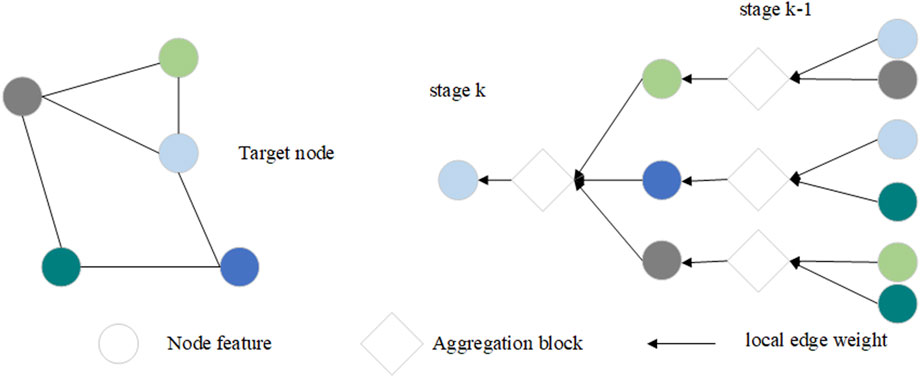
FIGURE 2. Sampling and aggregation process.

Figure 3 shows the design of the node-embedding module as well as the dense layers for TSP and QRP. The multi-head attention mechanism considers the global and local structure by weighing the more important nodes. The three-layer structure, input-size, and out-size for each layer are designed according to the node numbers per graph and the dimension of node features.

FIGURE 3

FIGURE 3. Structure of GraphSAGE-A.

3.4 TSP and QRP in dense

The output of the node-embedding module is concatenated by the outputs ${\mathrm{H}}_{\mathrm{m}}^{\mathrm{L}}$ of the three graphs for the $\mathrm{K}-\text{th}$ sample as follows:

${\overline{\mathrm{H}}}_{\mathrm{K}}=\text{CONCAT}\left({\mathrm{H}}_{\mathrm{m}}^{\mathrm{L}}\right),\mathrm{m}=\mathrm{1,2,3}.(13)$

Finally, the embedding matrix is formed as a vector, which is processed by full-connect multi-layer perceptron (MLP) modules: TSP and QRP. TSP refers to the classification task, whereas QRP refers to the regression task. We adopt the softmax and softsign functions for the output of TSP and QRP as (14) and (15), respectively.

${\widehat{\mathrm{p}}}_{\mathrm{i}}=\frac{\exp \left({\mathrm{z}}_{\mathrm{i}}^{\text{TSP}}\right)}{{\displaystyle {\sum }_{\mathrm{i}}}\exp \left({\mathrm{z}}_{\mathrm{i}}^{\text{TSP}}\right)},(14)$

$\widehat{\mathrm{v}}=\frac{{\mathrm{z}}^{\text{QRP}}}{1+\left|{\mathrm{z}}^{\text{QRP}}\right|}.(15)$

The confidence ${\widehat{\mathrm{p}}}_{\mathrm{i}}$ refers to the $\mathrm{i}-\text{th}$ category, while $\widehat{\mathrm{v}}$ denotes the predicted stability risk index.

3.5 A transient stability risk index

There is a three-dimensional label for each sample input in the GraphSAGE-A. The first and second dimensions of one-hot label refer to the TSP task via a trajectory-wise TSI as follows (Rahmatian et al., 2017):

${\text{TSI}}_{\mathrm{K}}=\frac{360°-{\left|{∆\mathrm{\delta }}_{\mathrm{m}\text{ax}}\right|}_{\mathrm{K}}}{360°+{\left|{∆\mathrm{\delta }}_{\mathrm{m}\text{ax}}\right|}_{\mathrm{K}}},(16)$

where ${\left|{∆\mathrm{\delta }}_{\mathrm{m}\text{ax}}\right|}_{\mathrm{K}}$ refers to the maximum rotor angle difference between any two generators during the sampling or simulation of the $\mathrm{K}-\text{th}$ sample. When ${\text{TSI}}_{\mathrm{K}}<0$, the $\mathrm{K}-\text{th}$ sample is unstable. Otherwise, the system is stable. It appears that the TSI defines a stability margin using a fixed value, while the TSB shifts slightly. Therefore, a transient stability RI is proposed to measure the stability deviation so that the special subsequent control schemes can be considered.

A fixed deviation ${∆}_{\mathrm{K}}$ of the $\mathrm{K}-\text{th}$ sample is defined as follows:

$\left.{\Delta }_{\mathrm{K}}=\left|\left(360\right.\right.°-{\left|{∆\mathrm{\delta }}_{\max }\right|}_{\mathrm{K}})\right|.(17)$

A normalized CCT is also considered as follows:

${\mathrm{t}}_{\mathrm{K}}^{*}=\frac{{\mathrm{t}}_{\mathrm{K}}-{\mathrm{\mu }}_{\text{CCT}}}{{\mathrm{\sigma }}_{\text{CCT}}},(18)$

where ${\mathrm{t}}_{\mathrm{K}}^{*}$ and ${\mathrm{t}}_{\mathrm{K}}^{*}$ refer to the normalized and original CTT of the $\mathrm{K}-\text{th}$ sample, respectively. ${\mathrm{\mu }}_{\text{CCT}}$ and ${\mathrm{\sigma }}_{\text{CCT}}$ denote the mean and standard deviation of the total dataset. Then, we developed an RI for the $\mathrm{K}-\text{th}$ sample as follows:

${\text{RI}}_{\mathrm{K}}=\left\{\begin{array}{cc}{\text{TSI}}_{\mathrm{K}}& {\Delta }_{\mathrm{K}}>{\mathrm{\delta }}_{\text{ts}}\\ \min \left(\text{sigmoid}\left({\mathrm{t}}_{\mathrm{K}}^{*}+\mathrm{\xi }\right)-1,{\text{TSI}}_{\mathrm{K}}\right)& {\Delta }_{\mathrm{K}}\le {\mathrm{\delta }}_{\text{ts}}\end{array}\right.,(19)$

where $\text{sigmoid}$ refers to the nonlinear activation function matching the strong nonlinearity and non-autonomy of the power system and ${\mathrm{\delta }}_{\text{ts}}$ denotes a discrimination threshold for the TSB shift among the samples of the training set. $\mathrm{\xi }$ considers the extreme cases, especially the multi-swing unstable samples. $\min$ selects the minimum value of inputs. The RI value is limited within the range of $\left[-\mathrm{1,1}\right]$ when proper ${\mathrm{\delta }}_{\text{ts}}$ approaches 0.

3.6 Loss function

Multi-task downstream networks, including the TSP task and the QRP task, share the output from node-embedding step as input. Evidently, the joint loss function of GraphSAGE-A consists of the loss from TSP and QRP. Additionally, a regularization item should be considered as follows:

$\text{LOSS}={\mathrm{L}}_{\text{TSP}}+{\mathrm{L}}_{\text{QRP}}+\mathrm{\beta }{\mathrm{L}}_{\mathrm{R}},(20)$

where the binary classification loss ${\mathrm{L}}_{\text{TSP}}$ is defined via the cross-entropy function with batch size $\mathrm{B}$ as follows:

${\mathrm{L}}_{\text{TSP}}=-\frac{1}{\mathrm{B}}{\displaystyle \sum _{\mathrm{b}}}\left[{\mathrm{o}}_1^{\mathrm{b}}\bullet \log \left({\widehat{\mathrm{p}}}_1^{\mathrm{b}}\right)+\left(1-{\mathrm{o}}_1^{\mathrm{b}}\right)\bullet \log \left(1-{\widehat{\mathrm{p}}}_1^{\mathrm{b}}\right)\right],(21)$

where $\left({\mathrm{o}}_0^{\mathrm{b}},{\mathrm{o}}_1^{\mathrm{b}}\right)$ is the one-hot label for the TSP task and ${\widehat{\mathrm{p}}}_{\mathrm{b}}=\left({\widehat{\mathrm{p}}}_0^{\mathrm{b}},{\widehat{\mathrm{p}}}_1^{\mathrm{b}}\right)$ denotes the stable possibility of the $\mathrm{b}-\text{th}$ sample. As for the regression loss ${\mathrm{L}}_{\text{QRP}}$, a mean squared error (MSE)-based function is utilized with batch size $\mathrm{B}$ as follows:

${\mathrm{L}}_{\text{QRP}}=-\frac{1}{\mathrm{B}}{\displaystyle \sum _{\mathrm{b}}}{\left({\widehat{\mathrm{\nu }}}_{\mathrm{b}}-{\text{RI}}_{\mathrm{b}}\right)}^2,(22)$

where ${\widehat{\mathrm{\nu }}}_{\mathrm{b}}$ and ${\text{RI}}_{\mathrm{b}}$ stand for the predicted and real RI of the ${\mathrm{b}}^{\text{th}}$ sample. We adopt the L2 function as the regularization item with weight $\mathrm{\beta }$. The Adam optimization is used for training.

3.7 Evaluation metrics

To evaluate the performance of the TSP task, we introduce the accuracy and f1-score metrics given by the following equations:

$\text{ACC}=\frac{{\mathrm{T}}_{\mathrm{P}}+{\mathrm{T}}_{\mathrm{N}}}{{\mathrm{T}}_{\mathrm{P}}+{\mathrm{T}}_{\mathrm{N}}+{\mathrm{F}}_{\mathrm{P}}+{\mathrm{F}}_{\mathrm{N}}}\times 100\%,(23)$

$\mathrm{F}1=\frac{2{\mathrm{T}}_{\mathrm{P}}}{{2\mathrm{T}}_{\mathrm{P}}+{\mathrm{F}}_{\mathrm{P}}+{\mathrm{F}}_{\mathrm{N}}}\times 100\%,(24)$

where ${\mathrm{T}}_{\mathrm{P}}$, ${\mathrm{T}}_{\mathrm{N}}$, ${\mathrm{F}}_{\mathrm{P}}$, and ${\mathrm{F}}_{\mathrm{N}}$, respectively, stand for the number of true positive, false negative, false positive, and false negative results. The MSE can evaluate the performance of the regressor. The formula is

$\text{MSE}=\frac{{\left({\widehat{\mathrm{\nu }}}_{\mathrm{b}}-{\text{RI}}_{\mathrm{b}}\right)}^2}{{\mathrm{T}}_{\mathrm{P}}+{\mathrm{T}}_{\mathrm{N}}+{\mathrm{F}}_{\mathrm{P}}+{\mathrm{F}}_{\mathrm{N}}}.(25)$

4 Experiments

4.1 Test system and simulation settings

The proposed MTTSA method is tested on the IEEE 39-bus system. As is shown in Figure 4, the total system consists of 39 buses, 10 generators, 19 loads, 34 transmission lines, and 12 transformers.

FIGURE 4

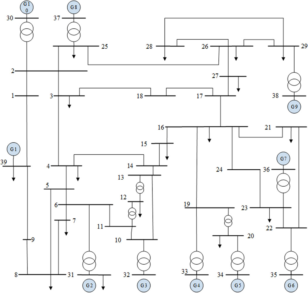
FIGURE 4. Topology of the IEEE 39-bus system.

All the samples are collected via TDS on PSD-BPA with sixth-order generator models. The loads are set as a proportional mix of the constant impedance and induction motor model. The settings of the simulation can be depicted as follows:

• Situations based on all transmission lines working are called the “Base” cases, while the “N-1” cases need one transmission line off by avoiding those cases with islands

• A total of 11 different load levels within 80%–120% are considered, while the generator outputs randomly match the power flow

• Three-phase grounding faults and two-phase grounding faults at the 0% of any transmission lines last for 0.1 s during every simulation lasting for 6 s

• Labels of each contingency for TSP and QRP can be collected and computed

Thus, 11,160 samples are selected with 5,929 stable ones and 5,231 unstable ones. The shuffled dataset is divided into the train set, validation set, and test set with a ratio of 3:1:1, respectively, to ensure the balance of distribution. All the experiments of the MTTSA method are conducted on a 64-bit computer with Intel(R) Core i7-12700 CPU@ 3.61 GHz CPU, 32 GB RAM, and NVIDIA GeForce RTX 3080Ti 12G GPU.

4.2 Tests on the multi-task training method

Figure 5 shows the effectiveness of the proposed multi-task training strategy with the same settings of the node-embedding module. The joint-training method clearly leads to a significant increase from three perspectives, including the ACC, F1-score, and MSE. The QRP mask promotes a clear instability risk from certain samples because enriched information was obtained from the multi-task training method.

FIGURE 5

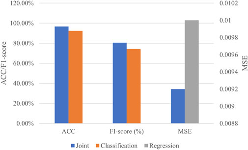
FIGURE 5. Performance of different strategies.

4.3 Hyperparameter testing in the GraphSAGE-A

For the whole structure of GraphSAGE-A, the multi-head attention aggregation is developed as the key physical-enhanced part. Regarding the hyperparameters, the number of heads $K$ and dropout rate $dropout$, both on the node features and the attention weights, respectively, are considered as the key parameters to be adjusted. During the tests of different parameter pairs, such as $K=\left(\mathrm{1,2,4,6,8}\right)$ and $dropout=\left(\mathrm{0,0.1,0.2,0.3,0.4,0.5}\right)$ (Figure 6), we find that each new setting brings enhanced performance on TSP and QRP, where the ACC and the F1-score increase by approximately 0.39% and 0.002%, respectively, while the MSE drops to 0.0068%. The optimal hyperparameter is selected as $K=6$ and $dropout=0.4$. All the hyperparameters of the model are shown in Table 2.

FIGURE 6

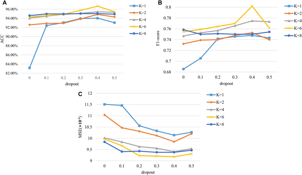
FIGURE 6. (A–C) Performance under various hyperparameters of the multi-head attention mechanism.

TABLE 2

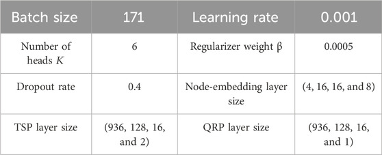
TABLE 2. Hyperparameters of GraphSAGE-A.

4.4 Verification of the multi-head attention structure

The local normalized edge weight method and the multi-head attention structure allow for more efficient adaptability to topology. In order to verify the improvement, the GraphSAGE-mean and each method detached GraphSAGE-A are compared to the proposed model with the same hyperparameter. The results are shown in Table 3. Essentially, adding both the single and simultaneous one as the developed model has shown significant profits compared to the baseline model.

TABLE 3

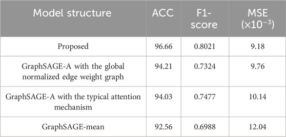
TABLE 3. Tests on the model structure verification.

4.5 Verification of RI

Figure 7 shows the distribution of CCT and RI of the uncertain samples when shifting TSB considered (${∆}_K\le {\mathrm{\delta }}_{ts}$) with settings of ${\mathrm{\delta }}_{ts}=15$, $\xi =2$ in (16). Apart from the stable samples, the nonlinear function can map samples located on the stable boundary to the appropriate range. The subsequent control strategies can be adopted for the power grid when the RI with suitable parameters is sufficiently small.

FIGURE 7

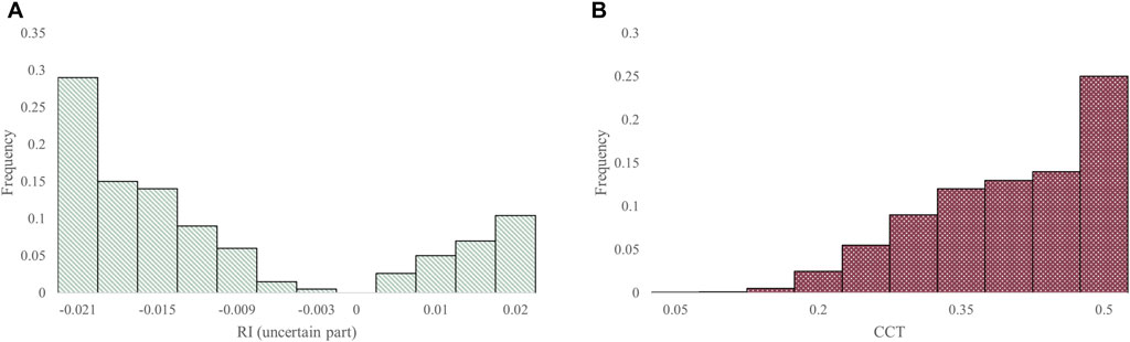
FIGURE 7. (A,B) Distribution of the RI (uncertain part) and CCT.

4.6 Comparison with baseline methods

We compare five baseline models with the proposed GraphSAGE-A method. Among them, CNN considers the feature-shaped 2D image as inputs, while LSTM adopts the raw inputs. The GNN-based models analyzed the same graph dataset with the three-layer node-embedding structure. Table 4 provides the results.

TABLE 4

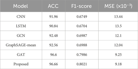
TABLE 4. Comparison with baseline methods on “Base” and “N-1.”

All the metrics of GraphSAGE-A performed better than the others, where ACC exceeds 96.66% and MSE decreases to 0.0092. The multi-head attention mechanism has been verified as a key factor for performance improvement, owing to its proper combination of global and local information.

Among the baseline methods, graph-deep structures such as GCN, GraphSAGE, and GAT stacked with topological processing show better performance than the traditional deep networks. Compared to GCN, the approximate structure of GraphSAGE-mean exhibits slight improvements across three metrics. Similarly, GraphSAGE-A also demonstrates slight improvements compared to GAT, which shares the multi-head attention structure.

4.7 Effectiveness analysis of the topological generalization ability

We further use the trained GraphSAGE-A in more samples from even worse conditions of the IEEE 39-bus system to test the generalization ability for the topology. The total 2,000 samples from “N-2” and “N-3” cases are selected with 960 stable and 1,040 unstable ones. The results are shown in Table 5.

TABLE 5

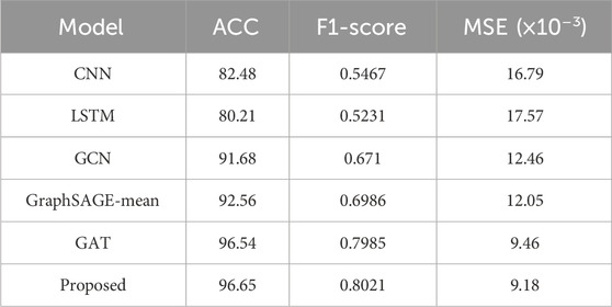
TABLE 5. Comparison with baseline methods on “N-2” and “N-3.”

Among the baseline models, traditional deep networks such as CNN and LSTM experience significant performance degradation when facing topological changes, where the ACC and F1-score decline by approximately 10% and 0.002% while the MSE drops to 0.017%. Due to the limitations in its inductive learning, GCN slightly decreases when facing topological changes. GraphSAGE, which considers reasoning and learning, GAT with introduced attention mechanism, and GraphSAGE-A, which simultaneously considers both, maintain stable performance. The results indicate that the method proposed in this paper outperforms other models in terms of adaptability to topology.

4.8 Analysis of unbalance distribution

A total of 500 samples from “Base,” “N-1,” “N-2,” and “N-3” cases are selected with 450 stable ones and 50 unstable ones to verify the extreme imbalance. A focal loss function is developed to rewrite the loss of TSP (Lin et al., 2017) as follows:

${\mathrm{L}}_{\text{TSP}}=-\frac{1}{\mathrm{B}}{\displaystyle \sum _{\mathrm{b}}}\left[\mathrm{\alpha }\bullet {\left.{\left(\mathrm{o}\right.}_1^{\mathrm{b}}\right)}^{\gamma }\bullet \log \left({\widehat{\mathrm{p}}}_1^{\mathrm{b}}\right)+\left(1-\mathrm{\alpha }\right)\bullet {\left(1-{\mathrm{o}}_1^{\mathrm{b}}\right)}^{\gamma }\bullet \log \left(1-{\widehat{\mathrm{p}}}_1^{\mathrm{b}}\right)\right],(26)$

where $\left({\mathrm{o}}_0^{\mathrm{b}},{\mathrm{o}}_1^{\mathrm{b}}\right)$ is the one-hot label for the TSP task and ${\widehat{\mathrm{p}}}_{\mathrm{b}}=\left({\widehat{\mathrm{p}}}_0^{\mathrm{b}},{\widehat{\mathrm{p}}}_1^{\mathrm{b}}\right)$ denotes the stable possibility of the $\mathrm{b}-\text{th}$ sample. $\alpha \in \left(\mathrm{0,1}\right)$ is a weighting factor for class $1$ and $1-\alpha$ is for class $0$. $\gamma \in \left[\mathrm{0,2}\right]$ is a value setting.

During the tests of different parameter pairs, such as $\alpha =\left(\mathrm{0.09,0.1,0.12,0.14,0.16}\right)$ and $\gamma =\left(\mathrm{0,0.5,1,1.5,2}\right)$ (Figure 8), the optimal hyperparameter is selected as $\alpha =0.12$ and $\gamma =1.5$. The performance under imbalance is maintained with a proper setting.

FIGURE 8

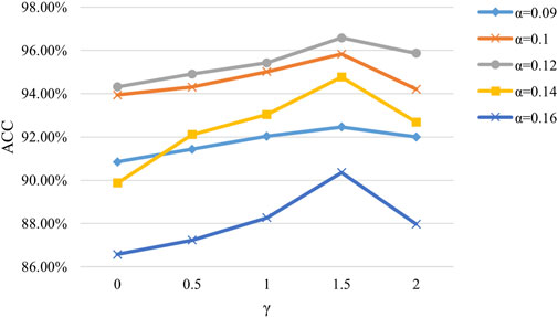
FIGURE 8. Performance under various hyperparameters of the focal loss function.

5 Conclusion

In this paper, an MTTSA method is adopted to detect the accurate TSP and QRP of power systems after faults. The system features from pre-fault, fault occurrence, and post-fault snapshots ($t_{0^{-}}$, $t_{0^{+}}$, and $t_{c^{+}}$) are transformed into multi-graph inputs. In addition to the transient stability binary analysis, the multi-task strategy allows the transient stability risks to be quantified and labeled by the RI, which considers the stability margin variability across various samples. During the joint-training stage, a topology adaptive network GraphSAGE-A is developed to learn the transient features, where a multi-head attention mechanism efficiently aggregates global information from the neighbors via proper weights. The extraction for contextual features is addressed by the local normalized strategy.

Therefore, tests based on the IEEE 39-bus system illustrate the obvious improvement of the proposed MTTSA method compared to baseline models. The adopted RI has been proved to quantify the transient stability risk considering the uncertain samples caused by TSB. Combined with the joint downstream, the risk of the power grid is rapidly calculated to guide the risk control strategies. Through the proper setting of credibility thresholds, the multi-head attention structure and the local normalization for edge weights are verified to be effective for model performance. Particularly, under severe topology variations, the MTTSA retains a steady precision and topology adaptive ability.

Further works will focus on optimizing the parameters of the model and improving the generalization ability for addressing more complex data.

Data availability statement

The raw data supporting the conclusion of this article will be made available by the authors, without undue reservation.

Author contributions

LH: conceptualization, methodology, writing–original draft, and writing–review and editing. KD: conceptualization, methodology, supervision, and writing–review and editing. JZ: writing–review and editing. KL: writing–review and editing. CJ: writing–review and editing. XG: writing–review and editing.

Funding

The authors declare that no financial support was received for the research, authorship, and/or publication of this article.

Conflict of interest

The authors declare that the research was conducted in the absence of any commercial or financial relationships that could be construed as a potential conflict of interest.

Publisher’s note

All claims expressed in this article are solely those of the authors and do not necessarily represent those of their affiliated organizations, or those of the publisher, the editors, and the reviewers. Any product that may be evaluated in this article, or claim that may be made by its manufacturer, is not guaranteed or endorsed by the publisher.

References

Chen, K., Hu, J., Zhang, Y., Yu, Z., and He, J. (2020). Fault location in power distribution systems via deep graph convolutional networks. IEEE J. Sel. Areas Commun. 38, 119–131. doi:10.1109/JSAC.2019.2951964

CrossRef Full Text | Google Scholar

Chen, Q., and Wang, H. (2021). Time-adaptive transient stability assessment based on gated recurrent unit. Int. J. Electr. Power Energy Syst. 133, 107156. doi:10.1016/j.ijepes.2021.107156

CrossRef Full Text | Google Scholar

Diao, R., Jin, S., Howell, F., Huang, Z., Wang, L., Wu, D., et al. (2017). On parallelizing single dynamic simulation using HPC techniques and APIs of commercial software. IEEE Trans. Power Syst. 32, 2225–2233. doi:10.1109/TPWRS.2016.2601024

CrossRef Full Text | Google Scholar

Ding, Y., Zhao, X., Zhang, Z., Cai, W., and Yang, N. (2022). Graph sample and aggregate-attention network for hyperspectral image classification. IEEE Geosci. Remote Sens. Lett. 19, 1–5. doi:10.1109/LGRS.2021.3062944

CrossRef Full Text | Google Scholar

Du, Y., and Hu, Z. (2021). Power system transient stability assessment based on snapshot ensemble LSTM network. Sustainability 13, 6953. doi:10.3390/su13126953

CrossRef Full Text | Google Scholar

Glavic, M., Ernst, D., Ruiz-Vega, D., Wehenkel, L., and Pavella, M. (2007). “E-SIME - a method for transient stability closed-loop emergency control: achievements and prospects,” in 2007 iREP Symposium - Bulk Power System Dynamics and Control - VII. Revitalizing Operational Reliability, Charleston, SC, USA, 19-24 August 2007 (IEEE), 1–10. doi:10.1109/IREP.2007.4410519

CrossRef Full Text | Google Scholar

Gomez, F. R., Rajapakse, A. D., Annakkage, U. D., and Fernando, I. T. (2011). Support vector machine-based algorithm for post-fault transient stability status prediction using synchronized measurements. IEEE Trans. Power Syst. 26, 1474–1483. doi:10.1109/TPWRS.2010.2082575

CrossRef Full Text | Google Scholar

Gupta, A., Gurrala, G., and Sastry, P. S. (2019). An online power system stability monitoring system using convolutional neural networks. IEEE Trans. Power Syst. 34, 864–872. doi:10.1109/TPWRS.2018.2872505

CrossRef Full Text | Google Scholar

Gurusinghe, D. R., and Rajapakse, A. D. (2016). Post-disturbance transient stability status prediction using synchrophasor measurements. IEEE Trans. Power Syst. 31, 3656–3664. doi:10.1109/TPWRS.2015.2496302

CrossRef Full Text | Google Scholar

Huang, J., Guan, L., Su, Y., Yao, H., Guo, M., and Zhong, Z. (2020). Recurrent graph convolutional network-based multi-task transient stability assessment framework in power system. IEEE Access 8, 93283–93296. doi:10.1109/ACCESS.2020.2991263

CrossRef Full Text | Google Scholar

Huang, J., Guan, L., Su, Y., Yao, H., Guo, M., and Zhong, Z. (2021). A topology adaptive high-speed transient stability assessment scheme based on multi-graph attention network with residual structure. Int. J. Electr. Power Energy Syst. 130, 106948. doi:10.1016/j.ijepes.2021.106948

CrossRef Full Text | Google Scholar

Ishizaki, T., Chakrabortty, A., and Imura, J.-I. (2018). Graph-theoretic analysis of power systems. Proc. IEEE 106, 931–952. doi:10.1109/JPROC.2018.2812298

CrossRef Full Text | Google Scholar

Kamwa, I., Samantaray, S. R., and Joos, G. (2012). On the accuracy versus transparency trade-off of data-mining models for fast-response PMU-based catastrophe predictors. IEEE Trans. Smart Grid 3, 152–161. doi:10.1109/TSG.2011.2164948

CrossRef Full Text | Google Scholar

Kim, C., Kim, K., Balaprakash, P., and Anitescu, M. (2019). “Graph convolutional neural networks for optimal load shedding under line contingency,” in 2019 IEEE Power and Energy Society General Meeting (PESGM), Atlanta, GA, USA, 04-08 August 2019 (IEEE), 1–5. doi:10.1109/PESGM40551.2019.8973468

CrossRef Full Text | Google Scholar

Li, X., Yang, Z., Guo, P., and Cheng, J. (2021). An intelligent transient stability assessment framework with continual learning ability. IEEE Trans. Ind. Inf. 17, 8131–8141. doi:10.1109/tii.2021.3064052

CrossRef Full Text | Google Scholar

Lin, H., Chen, Z., Chen, J., and Chen, W. (2022). “Transient stability analysis of AC-DC hybrid power grid under topology changes based on deep learning,” in 2022 12th International Conference on Power and Energy Systems (ICPES), Guangzhou, China, 23-25 December 2022 (IEEE), 514–519. doi:10.1109/ICPES56491.2022.10073461

CrossRef Full Text | Google Scholar

Lin, T.-Y., Goyal, P., Girshick, R., He, K., and Dollár, P. (2017). Focal loss for dense object detection. Proc. IEEE Int. Conf. Comput. Vis. 42, 318–327. doi:10.1109/tpami.2018.2858826

CrossRef Full Text | Google Scholar

Liu, S., Liu, L., Fan, Y., Zhang, L., Huang, Y., Zhang, T., et al. (2020). An integrated scheme for online dynamic security assessment based on partial mutual information and iterated random forest. IEEE Trans. Smart Grid 11, 3606–3619. doi:10.1109/TSG.2020.2991335

CrossRef Full Text | Google Scholar

Liu, X., Min, Y., Chen, L., Zhang, X., and Feng, C. (2021). Data-driven transient stability assessment based on kernel regression and distance metric learning. J. Mod. Power Syst. Clean. Energy 9, 27–36. doi:10.35833/MPCE.2019.000581

CrossRef Full Text | Google Scholar

Mahato, N. K., Dong, J., Song, C., Chen, Z., Wang, N., Ma, H., et al. (2021). “Electric power system transient stability assessment based on Bi-LSTM attention mechanism,” in 2021 6th Asia Conference on Power and Electrical Engineering (ACPEE), Chongqing, China, 08-11 April 2021 (IEEE), 777–782. doi:10.1109/ACPEE51499.2021.9437089

CrossRef Full Text | Google Scholar

Maria, G. A., Tang, C., and Kim, J. (1990). Hybrid transient stability analysis (power systems). IEEE Trans. Power Syst. 5, 384–393. doi:10.1109/59.54544

CrossRef Full Text | Google Scholar

Mukherjee, R., and De, A. (2020). Development of an ensemble decision tree-based power system dynamic security state predictor. IEEE Syst. J. 14, 3836–3843. doi:10.1109/JSYST.2020.2978504

CrossRef Full Text | Google Scholar

Rahmatian, M., Chen, Y. C., Palizban, A., Moshref, A., and Dunford, W. G. (2017). Transient stability assessment via decision trees and multivariate adaptive regression splines. Electr. Power Syst. Res. 142, 320–328. doi:10.1016/j.epsr.2016.09.030

CrossRef Full Text | Google Scholar

Senyuk, M., Safaraliev, M., Kamalov, F., and Sulieman, H. (2023). Power system transient stability assessment based on machine learning algorithms and grid topology. Mathematics 11, 525. doi:10.3390/math11030525

CrossRef Full Text | Google Scholar

Shi, Z., Yao, W., Zeng, L., Wen, J., Fang, J., Ai, X., et al. (2020). Convolutional neural network-based power system transient stability assessment and instability mode prediction. Appl. Energy 263, 114586. doi:10.1016/j.apenergy.2020.114586

CrossRef Full Text | Google Scholar

Siddiqui, S. A., Verma, K., Niazi, K. R., and Fozdar, M. (2018). Real-time monitoring of post-fault scenario for determining generator coherency and transient stability through ANN. IEEE Trans. Ind. Appl. 54, 685–692. doi:10.1109/TIA.2017.2753176

CrossRef Full Text | Google Scholar

Xu, Y., Dong, Z. Y., Zhang, R., Xue, Y., and Hill, D. J. (2015). A decomposition-based practical approach to transient stability-constrained unit commitment. IEEE Trans. Power Syst. 30, 1455–1464. doi:10.1109/TPWRS.2014.2350476

CrossRef Full Text | Google Scholar

Yan, R., Geng, G., and Jiang, Q. (2021). Data-driven transient stability boundary generation for online security monitoring. IEEE Trans. Power Syst. 36, 3042–3052. doi:10.1109/TPWRS.2020.3042210

CrossRef Full Text | Google Scholar

Yu, J. J. Q., Hill, D. J., Lam, A. Y. S., Gu, J., and Li, V. O. K. (2018). Intelligent time-adaptive transient stability assessment system. IEEE Trans. Power Syst. 33, 1049–1058. doi:10.1109/TPWRS.2017.2707501

CrossRef Full Text | Google Scholar

Zhan, X., Han, S., Rong, N., Liu, P., and Ao, W. (2022). A Two-Stage transient stability prediction method using convolutional residual memory network and gated recurrent unit. Int. J. Electr. Power Energy Syst. 138, 107973. doi:10.1016/j.ijepes.2022.107973

CrossRef Full Text | Google Scholar

Zheng, L., Hu, W., Hou, K., Xu, X., and Shao, G. (2017). “Real-time transient stability assessment based on deep recurrent neural network,” in 2017 IEEE Innovative Smart Grid Technologies - Asia (ISGT-Asia), Auckland, New Zealand, 04-07 December 2017 (IEEE), 1–5. doi:10.1109/ISGT-Asia.2017.8378321

CrossRef Full Text | Google Scholar