Harmonic state estimation and localization based on broad-band measurement

Harmonic and power quality issues brought by the high power electronics penetration level have become a rising threat to power grids. To achieve accurate measurement of the broadband harmonics caused by the power electronic devices, the broadband phasor measurement unit has been developed and installed. However, due to its high cost, it is less practical to install bPMU on each node, and therefore, how to obtain the global harmonic state in the power grid with minimum bPMUs is a crucial issue. This paper is focused on the harmonic state estimation method based on bPMU data. The mathematical model for harmonic state estimation is first derived based on circuit principles. Then, the weighted least squares method is then utilized to solve the established measurement equations for harmonic state estimation to obtain the harmonic state across the grid. Furthermore, the 0–1 integer programming approach is employed to optimize the installation locations of the bPMUs to reduce the overall cost while maintaining full observability. Subsequently, the harmonic sources are localized by analyzing the injected harmonic power on each node. Finally, the validity and effectiveness of the proposed method are proved by matching results between the proposed methods and the simulation model based on the IEEE 14-node system.

1 Introduction

The conventional AC power grid is experiencing a shift toward an AC-DC hybrid one with the continuous integration of the power electronics HVDC transmission projects. Meanwhile, large quantities of renewable energy generation units, e.g., PV panels and wind turbines, have been installed to meet the carbon peaking and carbon neutrality goals, which both necessitate power electronic converters to achieve energy integration (Xiao et al., 2021). Despite enhancing the controllability and flexibility of the power grids, the massive application of power electronic devices has also raised considerable harmonic issues, leading to a series of problems, such as deteriorated power quality, increased energy losses, accelerated equipment aging, etc (Xiao et al., 2018). Due to the nonlinearity of power electronics devices, the power grid harmonics have shown broadband and multi-source characteristics, which challenge the effectiveness of conventional harmonic measurement techniques. Therefore, it becomes imperative to accurately perceive the harmonic state across the power grid and locate the harmonic sources. These prerequisites are essential for implementing power quality enhancement measures and ensuring the safe, reliable, and stable operation of the power grid (Liang et al., 2010).

The concept of harmonic state estimation was initially proposed by Heydt in 1989, which immediately garnered the interest and enthusiastic discussion of numerous scholars (Heydt, 1989). The development of synchronized phasor measurement technology significantly broadened the range of available measurement quantities. In (Meliopoulos et al., 1994), the voltage and current phasors were chosen as the measured quantities, and harmonic voltage was selected as the state variable. A least squares estimation method with a certain level of universality was proposed. However, this method necessitates a substantial amount of redundant measurement data, resulting in a significant increase in computational burden and cost. Consequently, it is not suitable for systems with a large number of complex busbars. To address this issue (Xu et al., 2006), put forth a harmonic state estimation algorithm based on singular value decomposition, which effectively estimates the harmonic state of the power grid in cases of incomplete observability without requiring excessive redundant measurement data. In order to enhance the accuracy of harmonic state estimation (Wang et al., 2018), introduced a dynamic harmonic state estimation model based on feature extraction of harmonic sources. This model employs wavelet filtering to extract the characteristic components of harmonic source fluctuations, utilizing slow fluctuation components for calculating the state transition matrix and fast fluctuation components for calculating the system noise covariance matrix. However, it is important to note that this model solely focuses on conventional harmonic sources and does not account for the numerous distributed new harmonic sources such as wind power and photovoltaics that are prevalent today. Carta et al. (2019); Carta et al. (2021) consider the sparse characteristics of harmonic source distribution and transform the solution problem of the underdetermined model into an l₀ norm or l₁ norm problem. They utilize compressive sensing algorithms to solve the underdetermined harmonic state estimation model, thereby reconstructing the harmonic injection current of the harmonic source.

To enhance the perception of the operational status of the power grid, numerous advanced sensors have been installed in the grid (Cao et al., 2023). In response to the challenges posed by harmonic issues and the wideband nature of grid harmonics, high-performance measurement devices such as wideband measurement devices have been developed and deployed. These devices enable accurate synchronous measurement of harmonics from the first to the 50th order, as well as the inter-harmonics within this range (Jin et al., 2022). This hardware foundation and data support have paved the way for further research on harmonic source localization. The broadband measurement device, commonly referred to as the broadband phasor measurement unit (bPMU), offers significant advantages in terms of synchronization and real-time performance, thanks to its precise timing based on the Global Positioning System. However, the cost of bPMUs remains relatively high, prompting increased attention toward achieving harmonic state estimation with the minimum number of bPMUs. Currently, two main methods are employed to optimize the configuration of bPMUs. The first method aims to maximize measurement redundancy while minimizing the number of bPMUs, with observability as the primary objective (Babu and Bhattacharyya, 2019). The second method focuses on achieving the best application performance (Zeng et al., 2021). Considering the importance of accuracy and cost-effectiveness in harmonic state estimation, this paper proposes the utilization of 0–1 integer programming to configure bPMU devices. Additionally, the weighted least squares method is employed for harmonic state estimation.

Besides, to accurately allocate harmonic responsibilities and address harmonic pollution, it is crucial to locate the numerous harmonic sources within the power grid and identify the origins of harmonic pollution. Harmonic source localization involves utilizing measurement devices to obtain harmonic voltage and current data, which is then analyzed to determine the location of each harmonic source. Existing methods for harmonic source localization can be broadly categorized into two groups. The first category focuses on a single node, where the primary harmonic source is identified at the Point of Common Coupling (PCC) based on the impact of harmonic distortion on both the system side and the user side. However, this method is not suitable for scenarios with multiple harmonic sources in practical power grids (Ding et al., 2020). The second category of methods is based on the results of harmonic state estimation, enabling the identification of multiple harmonic sources across the entire network (Yu et al., 2019). This approach provides a foundation for effective harmonic management and has emerged as a new research area in the context of multi-source harmonics in power grids. Chen and Shao. (2019) proposed a harmonic source localization method based on maximum a posteriori estimation, which requires a reduced number of measurement devices and effectively reduces measurement noise interference. In (Zhang et al., 2021), the authors differentiate between harmonic and non-harmonic sources by exploiting the linear and nonlinear differences in the equivalent models of these sources. A harmonic source localization method based on modal identification is proposed, which identifies the harmonic source by calculating the conformity between the measured electrical quantities and the linear model. However, this method requires power quality monitoring data from each load-supply line, which is difficult to obtain in practical applications. To address the issue of local unobservable systems (Shao et al., 2023), present a harmonic source localization method based on interval dynamic state estimation. The unobservable system is transformed into an equivalent observable system, and the Unscented Bayesian Interacting Kalman Filter (UBIKF) algorithm is utilized for harmonic state estimation, which accurately determines the location of harmonic sources within the unobservable area.

This article is focused on harmonic state estimation and source location based on bPMU measurement data. The mathematical model for harmonic state estimation is first derived based on circuit principles. The weighted least squares method is then utilized to solve the established measurement equations for harmonic state estimation to obtain the harmonic state across the grid. Furthermore, the 0–1 integer programming approach is employed to optimize the installation locations of the bPMUs to reduce the overall cost. Subsequently, the harmonic sources are localized by analyzing the injected harmonic power on each node. Finally, a simulation model is constructed in MATLAB based on the IEEE 14-bus system, and the validity and effectiveness of the proposed method are proved by matching results between the proposed methods and the model. This simulation serves as a means to assess the correctness of the estimation and localization methods, ensuring their reliability in practical power system scenarios. Overall, this research paper contributes to the advancement of harmonic analysis and management in power systems, offering valuable insights into mathematical modeling, estimation techniques, and source localization methodologies.

2 Harmonic state estimation

Harmonic state estimation primarily consists of three steps: the selection of measurement quantities and state variables, the establishment of the measurement matrix, and the solution of the mathematical model. The basic block diagram is illustrated in Figure 1.

FIGURE 1

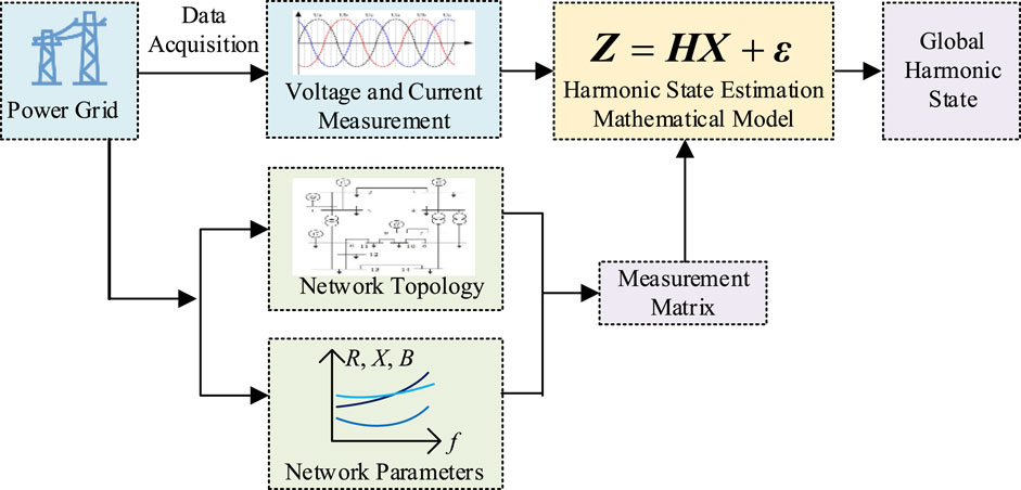
FIGURE 1. Structure diagram of harmonic state estimation.

2.1 Harmonic state estimation phasor measurement equations

2.1.1 Node voltage measurement equations

The node voltage measurement equations utilize node harmonic voltage phasors as measurement quantities to estimate the harmonic voltages at nodes during harmonic conditions. The measurement equation is expressed as follows:

${\dot{\mathit{U}}}_{\mathit{M},\mathit{i}}^{\mathit{h}}=\mathit{I}{\dot{\mathit{U}}}_{\mathit{S},\mathit{i}}^{\mathit{h}}+{\mathit{\eta }}_{\mathit{i}}(1)$

where the subscript M and S represent the measurement and the state quantities, respectively; ${\dot{U}}_{M,i}^h$ denotes the h-th harmonic voltage measurement at node i; ${\dot{U}}_{S,i}^h$ represents the h-th harmonic voltage state quantity at node i; I is the identity matrix with dimensions matching the voltage measurement, and ${\eta }_i$ signifies the measurement error at node i under h-th harmonic conditions.

2.1.2 Node current injection measurement equations

According to Kirchhoff’s current law, the sum of currents flowing out of any node is always equal to the sum of currents flowing into it. Utilizing this principle, the harmonic injection current at the measurement device node can be selected as a measurement quantity. By considering the network topology structure and component harmonic parameters, the harmonic voltages at other nodes can be determined. The measurement equation is expressed as follows:

${\dot{\mathit{I}}}_{\mathit{M},\mathit{i}}^{\mathit{h}}=\sum _{\mathit{j}=\mathbf{1}}^{\mathit{n}}{\dot{\mathit{Y}}}_{\mathit{i}\mathit{j}}^{\mathit{h}}{\dot{\mathit{U}}}_{\mathit{S},\mathit{j}}^{\mathit{h}}+{\mathit{\eta }}_{\mathit{i}}(2)$

Where, ${\dot{I}}_{M,i}^h$ represents the h-th harmonic current injection measurement at node I; ${\dot{U}}_{S,j}^h$ denotes the h-th harmonic voltage state quantity at node j; ${\dot{Y}}_{ij}^h$ represents the matrix element in the admittance matrix of nodes i and j related to the h-th harmonic under the given conditions, and n represents the total number of nodes in the tested system.

2.1.3 Branch current injection measurement equations

If a broadband measurement device is installed at node i, the current in the branches connected to node i can be used as a measurement quantity, which is referred to as branch current injection measurement.

Based on the π-type equivalent harmonic model of the transmission line or transformer branch shown in Figure 2, the measurement equation for branch currents can be established as follows:

${\dot{\mathit{I}}}_{\mathit{M},\mathit{i}\mathit{j}}^{\mathit{h}}={\mathit{Y}}_{\mathit{i}\mathit{i}}^{\mathit{h}}{\dot{\mathit{U}}}_{\mathit{S},\mathit{i}}^{\mathit{h}}+{\mathit{Y}}_{\mathit{i}\mathit{j}}^{\mathit{h}}{\dot{\mathit{U}}}_{\mathit{S},\mathit{j}}^{\mathit{h}}+{\mathit{\eta }}_{\mathit{i}}=\left({\mathit{y}}_{\mathit{i}\mathit{i}}^{\mathit{h}}+{\mathit{y}}_{\mathit{i}\mathit{j}}^{\mathit{h}}\right){\dot{\mathit{U}}}_{\mathit{S},\mathit{i}}^{\mathit{h}}-{\mathit{y}}_{\mathit{i}\mathit{j}}^{\mathit{h}}{\dot{\mathit{U}}}_{\mathit{S},\mathit{j}}^{\mathit{h}}+{\mathit{\eta }}_{\mathit{i}}={\mathit{y}}_{\mathit{i}\mathit{i}}^{\mathit{h}}{\dot{\mathit{U}}}_{\mathit{S},\mathit{i}}^{\mathit{h}}+{\mathit{y}}_{\mathit{i}\mathit{j}}^{\mathit{h}}\left({\dot{\mathit{U}}}_{\mathit{S},\mathit{i}}^{\mathit{h}}-{\dot{\mathit{U}}}_{\mathit{S},\mathit{j}}^{\mathit{h}}\right)+{\mathit{\eta }}_{\mathit{i}}(3)$

FIGURE 2

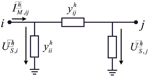
FIGURE 2. Equivalent circuit of transmission line and transformer.

Where, ${\dot{I}}_{M,ij}^h$ represents the measurement quantity of the injected current between node i and node j under hth harmonic conditions; ${\dot{U}}_{S,i}^h$ denotes the harmonic voltage at node i under hth harmonic conditions; ${\dot{U}}_{S,j}^h$ represents the harmonic voltage at node j under hth harmonic conditions; $Y_{ii}^h=y_{ii}^h+y_{ij}^h$, $Y_{ij}^h=-y_{ij}^h$, and $y_{ii}^h$ represent the self-admittance in the admittance matrix of node i under hth harmonic conditions, and $y_{ij}^h$ signifies the admittance between node i and node j under hth harmonic conditions.

2.2 Mathematical model for harmonic state estimation

Harmonic state estimation involves developing a mathematical model that relates the measurement quantities to the state quantities. This is commonly accomplished by incorporating current measurements, voltage measurements, or their derivatives. By applying the fundamental principles of circuit theory, a fundamental mathematical model for harmonic state estimation can be formulated.

In this paper, the measurement quantities selected for harmonic state estimation are the harmonic voltages at nodes and the harmonic currents in branches. Additionally, the harmonic currents at nodes are chosen as the state quantities. The modified equation for the branch current injection measurement variation is presented as Equation 4, and the synchronized phasor measurement equation is established as Equation 5:

${\dot{\mathit{I}}}_{\mathit{M},\mathit{i}\mathit{j}}^{\mathit{h}}={\mathit{y}}_{\mathit{i}\mathit{i}}^{\mathit{h}}{\dot{\mathit{U}}}_{\mathit{S},\mathit{i}}^{\mathit{h}}+{\mathit{y}}_{\mathit{i}\mathit{j}}^{\mathit{h}}\left({\dot{\mathit{U}}}_{\mathit{S},\mathit{i}}^{\mathit{h}}-{\dot{\mathit{U}}}_{\mathit{S},\mathit{j}}^{\mathit{h}}\right)=\left[\left({\dot{\mathit{y}}}_{\mathit{i}\mathit{i}}^{\mathit{h}}+{\dot{\mathit{y}}}_{\mathit{i}\mathit{j}}^{\mathit{h}}\right){\dot{\mathit{Z}}}_{\mathit{i}}^{\mathit{h}}-{\dot{\mathit{y}}}_{\mathit{i}\mathit{j}}^{\mathit{h}}{\dot{\mathit{Z}}}_{\mathit{j}}^{\mathit{h}}\right]{\dot{\mathit{I}}}_{\mathit{S}}^{\mathit{h}}(4)$

$\left[\begin{array}{c}{\dot{\mathit{U}}}_{\mathit{M}}^{\mathit{h}}\\ {\dot{\mathit{I}}}_{\mathit{M},\mathit{i}\mathit{j}}^{\mathit{h}}\end{array}\right]=\left[\begin{array}{c}{\dot{\mathit{H}}}_{\mathbf{1}}\\ {\dot{\mathit{H}}}_{\mathbf{2}}\end{array}\right]{\dot{\mathit{I}}}_{\mathit{S}}^{\mathit{h}}(5)$

Where, ${\dot{U}}_M^h$ denotes the measurement of the harmonic voltage at the node where the bPMU device is installed; ${\dot{I}}_{M,ij}^h$ represents the measurement of harmonic current in the branch connected to the node where the bPMU device is installed; ${\dot{I}}_S^h$ represents the unknown harmonic current state at each node; ${\dot{H}}_1$ represents the measurement matrix where the measurement quantity is the harmonic voltage at the node; ${\dot{H}}_2$ represents the measurement matrix where the measurement quantity is the harmonic current in the branch; ${\dot{U}}_{S,i}^h$ represents the harmonic voltage at node i under hth harmonic conditions; ${\dot{U}}_{S,j}^h$ represents the harmonic voltage at node j under hth harmonic conditions; $y_{ii}^h$ represents the self-admittance in the admittance matrix of node i under hth harmonic conditions, and $y_{ij}^h$ represents the admittance between node i and node j under hth harmonic conditions.

Based on the phasor measurement equations in Section 2.1, by observing the form of Equation 5, the mathematical model can be defined as follows:

$\mathit{Z}=\mathit{H}\mathit{X}+\mathit{\epsilon }(6)$

Where, Z is an m × 1-dimensional vector representing the measurement phasors; X is an n × 1-dimensional vector representing the unknown state phasors; Z and X are determined based on the selected measurement and state quantities and the phasor measurement equations; H is an m×n-dimensional measurement matrix that serves as a bridge connecting the measurement quantities and the state quantities; the measurement matrix is mainly determined by the network topology and the harmonic parameters of the components in the tested power system, ε represents an m × 1-dimensional vector representing the measurement error; m represents the number of measurement quantities, and n represents the number of unknown state quantities.

2.3 Harmonic source localization

Based on harmonic state estimation, the localization of harmonic sources involves identifying whether a node injects positive or negative harmonic active power into the system. This determination helps in classifying the node as a harmonic source or a harmonic absorption source. If a node injects positive harmonic active power, it is categorized as a harmonic injection source. Conversely, if it injects negative harmonic active power, it is considered a harmonic absorption source. Assuming that the harmonic current in the entire study area has been estimated through harmonic state estimation, the harmonic voltages at each node can be obtained using Equation 2.

The injected harmonic active power at the ith node for the hth harmonic is defined as follows:

${\mathit{P}}_{\mathit{i}}^{\mathit{h}}=\mathit{R}\mathit{e}\left({\dot{\mathit{U}}}_{\mathit{i}}^{\mathit{h}}\stackrel{*}{{\dot{\mathit{I}}}_{\mathit{i}}^{\mathit{h}}}\right)(7)$

where ${\dot{U}}_i^h$ represents the harmonic voltage at the node; $\stackrel{*}{{\dot{I}}_i^h}$ represents the complex conjugate of the harmonic current at the node. The sign of the injected active power is used to determine whether the node is a harmonic source.

2.4 Harmonic source localization based on weighted least squares estimation

The solution to the harmonic state estimation model is essentially the solution to the objective function, which aims to calculate the optimal estimate based on the selected estimation criterion. Both the measurement characteristics of the synchronized phasor measurement device and the constructed mathematical model are linear. The harmonic state estimation model is solved using the weighted least squares estimation method, which improves the distribution of errors among different measurement data. The mathematical model for harmonic state estimation, as presented in Equation 6, shows that Equation 8 represents the measurement estimation error vector, while Equation 9 represents the objective function of the weighted least squares method. The weighted least squares method weights the original model to make it a model without heteroscedasticity. Then, it estimates its parameters using the least squares method to obtain the optimal solution of the objective function.

$v=\mathit{H}\widehat{\mathit{X}}-\mathit{Z}(8)$

$J\left(x\right)={\left(\mathit{Z}-\mathit{H}\mathit{X}\right)}^T\mathit{W}\left(\mathit{Z}-\mathit{H}\mathit{X}\right)(9)$

Where, $\widehat{X}$ represents the estimated value of the state variable X.

When $\mathit{X}=\widehat{\mathit{X}}$, the objective function reaches its minimum value, that is:

$\mathit{min}J\left(x\right)={\left(\mathit{Z}-\mathit{H}\mathit{X}\right)}^T\mathit{W}\left(\mathit{Z}-\mathit{H}\mathit{X}\right)(10)$

To find the minimum value of the sum of squared residuals, the harmonic state estimation equation based on the weighted least squares principle is derived:

${\mathit{H}}^T\mathit{W}\mathit{H}\widehat{\mathit{X}}={\mathit{H}}^T\mathit{W}\mathit{Z}(11)$

where $\mathit{W}={\mathit{R}}^{-1}$; W is the m×m-dimensional measurement weight matrix; R is the diagonal matrix of error variances for each measurement data.

Solving Equation 11 yields the weighted least squares solution for the harmonic state estimation model:

$\widehat{\mathit{X}}={\left({\mathit{H}}^T\mathit{W}\mathit{H}\right)}^{-1}{\mathit{H}}^T\mathit{W}\mathit{Z}(12)$

3 Observability analysis and broadband measurement device configuration

3.1 Integer programming mathematical model

The observability of a power system refers to the availability of sufficient measurement data to determine the state of the entire network. A node is considered observable if its state is known or can be calculated. Currently, there are two perspectives on defining network observability: algebraic and topological (Han et al., 2022). Based on the fundamental principles of circuits, nodes equipped with broadband measurement devices not only provide voltage information but also enable the determination of branch currents connected to those nodes. As a result, both the nodes with broadband measurement devices and their adjacent nodes become observable.

In this research paper, the configuration of broadband measurement devices is addressed as a 0–1 integer programming problem to achieve system observability while minimizing the number of devices required. The variable "x" is used to indicate whether a node is equipped with a broadband measurement device, where x = 1 denotes the presence of a device at a node and x = 0 signifies its absence. The intlinprog function is commonly used to solve the 0–1 integer programming problem on the MATLAB simulation platform. Eq. 13 represents the standard form of this function.

$\underset{x}{\mathit{min}}{\mathit{f}}^{\mathit{T}}x$

$s.t.\left\{\begin{array}{c}x\left(\text{intcon}\right)\text{is\hspace{0.17em}an\hspace{0.17em}integer}\\ \mathit{A}\cdot x\le b\\ \mathit{A}\mathit{e}\mathit{q}\cdot x=\mathit{b}\mathit{e}\mathit{q}\\ lb\le x\le ub\end{array}\right.(13)$

Here, A and b are coefficient matrices in the inequality constraints; Aeq and beq are coefficient matrices in the equality constraints; lb and ub represent the upper and lower bounds of each variable, and $\mathit{f}$ represents the coefficient matrix of each variable in the objective function.

The 0–1 integer programming mathematical model for PMU configuration in an n-node system is as follows:

$\mathit{min}{\displaystyle \sum _{i=1}^n}{x}_i$

$s.t.\left\{\begin{array}{c}\mathit{A}\cdot \mathit{X}\ge \mathit{I}\\ x_i=0\text{or\hspace{0.17em}}1\end{array}\right.(14)$

where $x_i=\left\{\begin{array}{c}1\\ 0\end{array}\right.\begin{array}{c}\text{Node\hspace{0.17em}}\mathrm{i}\text{\hspace{0.17em}configures\hspace{0.17em}the\hspace{0.17em}bPMU}\\ \text{Node\hspace{0.17em}}\mathrm{i}\text{\hspace{0.17em}is\hspace{0.17em}not\hspace{0.17em}configured\hspace{0.17em}with\hspace{0.17em}bPMU}\end{array}i=1,2,\cdots ,n$, A is the node adjacency matrix of the system, taking a value of 1 when there is a connection between two nodes and 0 otherwise; $\mathit{X}={\left(x_1,x_2,\cdots ,x_n\right)}^T$; $I={\left(\mathrm{1,1},\cdots ,1\right)}^T$.

3.2 Solving the 0–1 integer programming mathematical model

According to the fundamental principles of circuits, when broadband measurement devices are installed at specific nodes, not only can the voltage at that node be known, but also the branch currents connected to it. As a result, both the nodes where broadband measurement devices are installed and their adjacent nodes become observable. To illustrate this concept, we utilize the IEEE 14-node system as a case study and construct an analysis table for broadband measurement device configuration. Figure 3 depicts the topology diagram of the IEEE 14-node system. In Table 1, the first column represents the nodes where broadband measurement devices are installed, while the first row indicates the nodes that become observable when a broadband measurement device is installed at the respective node listed in the first column. A value of "1"in the table signifies that the corresponding node is observable. For instance, taking node 2 in the IEEE 14-node system as an example, according to Figure 3, nodes 1, 3, 4, and 5 are all connected to node 2. Therefore, in Table 1, the observable nodes 1, 2, 3, 4, and 5 are marked with the digit "1"after a broadband measurement device is installed at node 2.

FIGURE 3

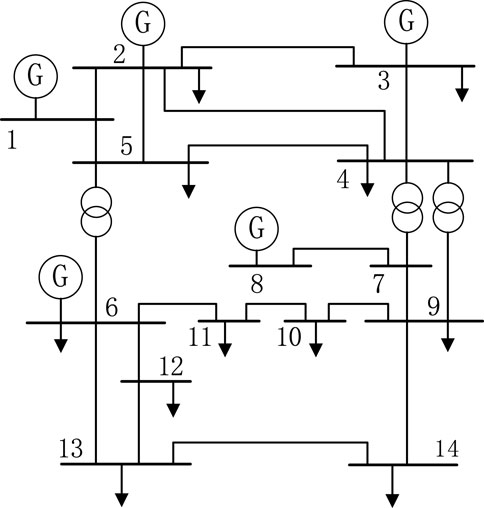
FIGURE 3. IEEE14 node system.

TABLE 1

TABLE 1. The bPMU configuration analysis table of IEEE14 node system.

To minimize costs, it is desirable to reduce the number of broadband measurement devices while ensuring the observability of the power system. To achieve this objective, we propose an objective function that can be represented by Equation 15:

$\mathit{min}\left(x_1+x_2+\cdots +x_{14}\right)(15)$

To achieve system observability, every node in the system must be observable. Based on the information provided in Table 1, a node can be made observable if either the node itself or at least one of its connected nodes is equipped with a broadband measurement device. For instance, in the case of node 2, it can be observed if any of the nodes 1, 3, 4, or 5 has a broadband measurement device installed. Consequently, the inequality constraints for the 0–1 integer programming formulation of the IEEE 14-node system can be derived as follows:

$\left\{\begin{array}{c}{x}_1+x_2+x_5\ge 1\\ x_1+x_2+x_3+x_4+x_5\ge 1\\ ⋮\\ x_9+x_{13}+x_{14}\ge 1\end{array}\right.(16)$

The objective function can be solved using the intlinprog function in MATLAB simulation, providing a configuration scheme for broadband measurement devices that ensures full observability of the system. For the IEEE 14-node system, the 0–1 programming yields the following positions for broadband measurement device configuration: nodes 2, 8, 10, and 13. Referring to Table 1, it can be confirmed that when these four nodes are equipped with broadband measurement devices, every node in the IEEE 14-node system becomes observable. Furthermore, each node has only one related node with a broadband measurement device, effectively minimizing the number of broadband measurement devices while ensuring system observability.

4 Simulation results and analysis

In this study, we validate a harmonic state estimation method using synchronized phasor measurements, employing the IEEE 14-node system as an example. The system comprises an AC load, two three-phase six-pulse converter terminals (LCC), and a modular multi-level converter terminal (MMC). Node 11 is connected to the AC load, while nodes 5 and 14 are connected to the LCC, and node 4 is connected to the MMC. The harmonic sources are simplified as harmonic current sources injecting harmonic currents into the system. The system’s topology relationship is depicted in Figure 4. To perform power flow calculations on the IEEE 14-node system, we utilize the MATLAB tool MATPOWER to obtain the power flow state at the fundamental frequency. The amplitudes and phase angles of each harmonic current are determined based on the typical spectrum of harmonic currents and the current at the fundamental frequency, the spectrum table of harmonic loads is shown in Table 2. (Xiao et al., 2021). This establishes the measurement and verification databases for harmonic state estimation. Under stable operating conditions of the AC-DC power grid, the AC grid primarily contains the 12k ± 1 (k = 1, 2, 3, … ) harmonic components, while the DC part mainly contains the 12k (k = 1, 2, 3, … ) harmonic components. However, the MMC-induced resonance frequency depends on various factors such as the equivalent impedance parameters of the port grid, its own control and topology parameters, and lacks numerical regularity. Therefore, for the sake of simplicity, this paper assumes that the harmonic current injected by the MMC is equivalent to a high-frequency harmonic current source with a frequency of 515 Hz. The amplitude of this harmonic current is set to 5% of the fundamental current. Given that higher-order harmonics have smaller amplitudes and lower significance, we focus on the 11th and 13th harmonics, which have the greatest impact, as well as the non-integer harmonics introduced by the MMC in the example.

FIGURE 4

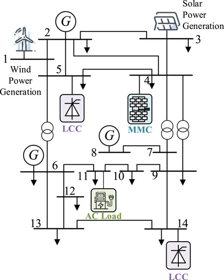
FIGURE 4. IEEE14 node AC/DC system.

TABLE 2

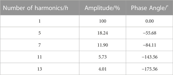
TABLE 2. Spectrum table of harmonic loads.

The algorithm flow is depicted in Figure 5. Initially, the harmonic order, h, is provided as input, and the measurement database for harmonic state estimation corresponding to the harmonic order is constructed. This involves extracting the necessary measurement data and verification from the broadband measurement devices. Using the constructed example, a 0–1 programming model is established to determine the optimal locations for the broadband measurement devices. Subsequently, the relevant data is extracted from the measurement database, and the h-order harmonic node admittance matrix is formed by combining it with the example. This matrix, denoted as H, is utilized for harmonic state estimation. The weighted least squares method is employed to solve the harmonic state estimation equations, yielding the estimated state values. These estimated values are then compared with the actual values to assess the accuracy of the harmonic state estimation. Building upon the accurate harmonic state estimation, the active power injection at each node is calculated. Based on the positive and negative values of active power injection at the nodes, the locations of the harmonic sources in the example are determined.

FIGURE 5

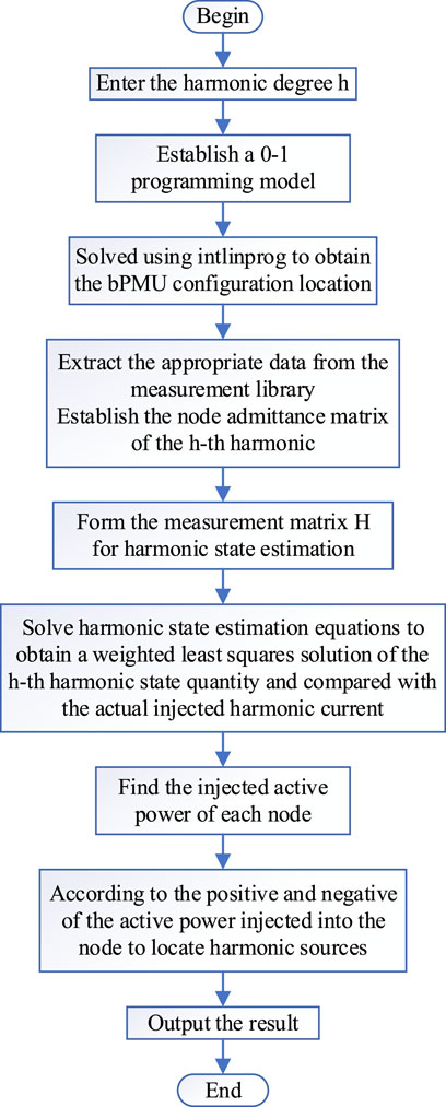
FIGURE 5. Flow chart of the proposed algorithm.

According to the 0–1 integer programming model, the optimal locations for the broadband measurement devices are determined to be node 2, node 8, node 10, and node 13. These nodes are selected to measure the harmonic voltages, while the harmonic currents at these nodes are considered as the state quantities. The data collected from the broadband measurement devices includes the harmonic voltage values at the installed nodes, as well as the harmonic current values of the branches connected to these nodes. Using this data, we construct the measurement matrices H for the 11th harmonic, 13th harmonic, and the non-integer harmonic introduced by the MMC.

Random measurement errors, with a mean of 0 and a standard deviation of 0.2%, are introduced into the broadband measurement data. The measurement equations are then formulated for the IEEE 14-node system, considering the 515 Hz, 11th harmonic, and 13th harmonic scenarios for the multi-harmonic source cases. By utilizing synchronized phasor measurements, the weighted least squares method is employed to solve the harmonic state estimation equations, resulting in the determination of the state quantities, specifically the harmonic currents at each node. In the case of the 515 Hz harmonic, our focus lies on the injected harmonic currents originating from the MMC. Conversely, for the 11th and 13th harmonics, our attention is directed towards the AC loads and LCC. The estimated deviations of the harmonic source nodes are presented in Tables 3–5.

TABLE 3

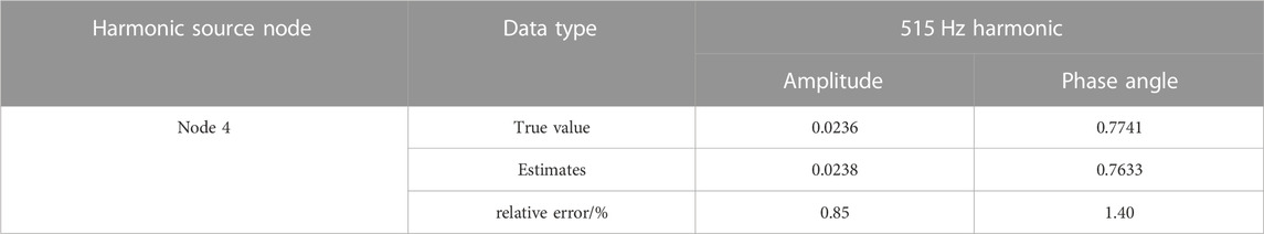
TABLE 3. Comparison result of 515 Hz harmonic current at the MMC harmonic source bus of IEEE14 system.

TABLE 4

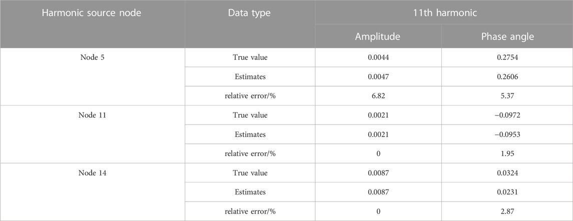
TABLE 4. Comparison result of 11th harmonic current at the harmonic source bus of IEEE14 system.

TABLE 5

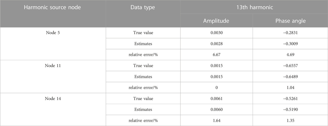
TABLE 5. Comparison result of 13th harmonic current at the harmonic source bus of IEEE14 system.

Based on the data presented in Tables 3–5, it can be observed that the average relative error of the harmonic state estimation for the 515 Hz, 11th harmonic, and 13th harmonic scenarios is consistently below 3% for the amplitude. This indicates a high level of estimation accuracy, exceeding 97% on average. Furthermore, the average relative error of the phase for the harmonic state estimation is also below 3.5%, demonstrating an average estimation accuracy of over 96.5%. These results highlight the effectiveness of the proposed harmonic state estimation method, which relies on broadband synchronized phasor measurements, in accurately determining the harmonic conditions of the IEEE 14-node system under multi-harmonic source scenarios.

Once the harmonic state estimation accurately determines the harmonic conditions within the system, the next step is to conduct further analysis for harmonic source localization. This process involves identifying whether the nodes inject positive or negative harmonic active power into the system. If a node injects positive harmonic active power, it is identified as a harmonic injection source. Conversely, if it injects negative harmonic active power, it is considered a harmonic absorption source.

The harmonic current values at each node can be obtained through harmonic state estimation, and using the node injection current equations, the harmonic voltage values at each node can be further determined. The harmonic active power at each node can be calculated using the formula presented in Table 6.

TABLE 6

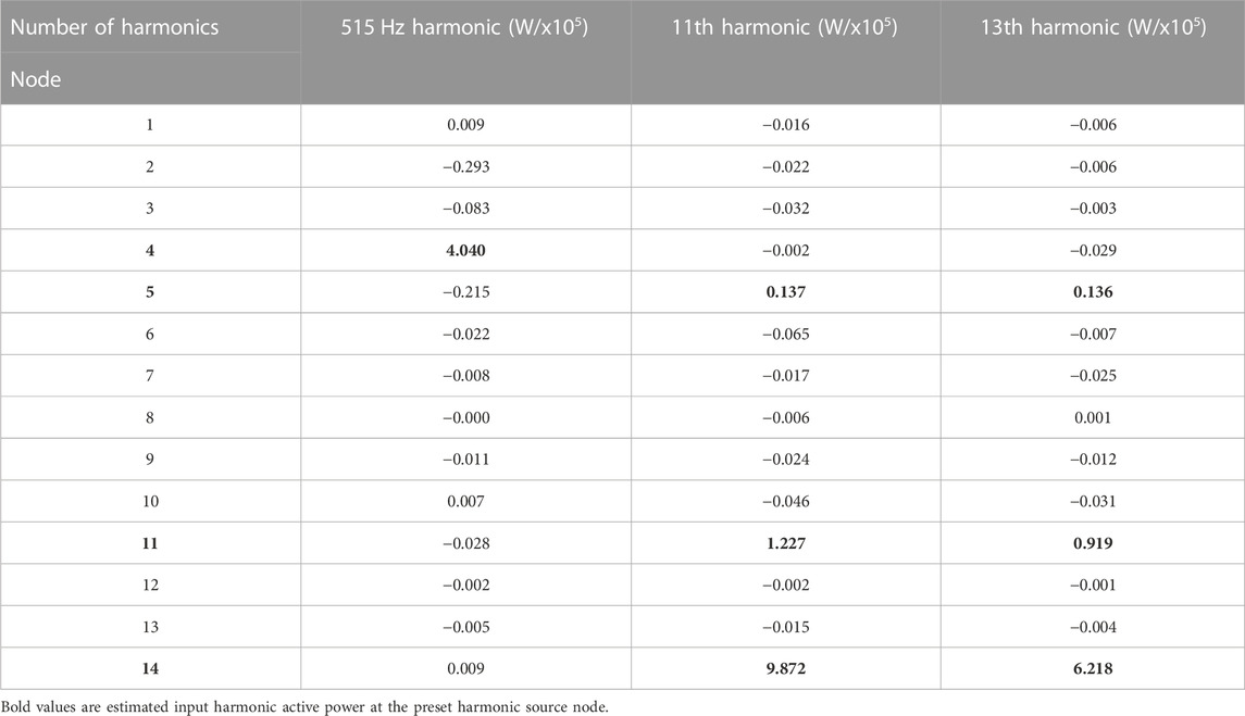
TABLE 6. Estimated value of nodal injection harmonic active power.

Based on the information presented in Table 3, it can be concluded that the system contains four harmonic sources located at nodes 4, 5, 11, and 14. Node 4 is identified as a non-integer multiple harmonic source at 515 Hz, while nodes 5, 11, and 14 are identified as harmonic sources at the 11th and 13th harmonics, consistent with the designated harmonic source scenarios. Additionally, a few individual nodes exhibit positive harmonic active power values. However, these values are negligible and fall within the acceptable range of measurement and estimation errors. Thus, the employed harmonic source localization method proves to be effective and accurate in identifying the harmonic sources in the system.

5 Conclusion

With the integration of numerous power electronic and renewable energy devices into the power grid, the issue of harmonic pollution has become increasingly severe. The sources of harmonics are becoming more diverse, and their detrimental impact on power quality is growing. This paper aims to address the coexistence of multiple harmonic sources to ensure the safe, stable, and reliable operation of the AC/DC hybrid grid. To achieve this, a harmonic state estimation method based on broadband synchronized phasor measurement is proposed. By capitalizing on the advantages of broadband measurement devices and employing a simple and comprehensible 0–1 integer programming concept for their configuration, the proposed method reduces the number of broadband measurement devices, mitigating their high cost and effectively lowering the overall expenses. With fewer broadband measurement devices, the proposed method can reliably estimate the harmonic conditions of the system, ensuring its observability. Furthermore, building upon the achievement of harmonic state estimation, this paper delves into the problem of harmonic source localization, accomplishing basic localization of harmonic sources within the system using the data obtained from harmonic state estimation.

Due to the limitations of experimental conditions, this paper only conducted numerical simulation verification of the proposed method using MATLAB. It was not possible to verify it on a semi-physical simulation platform. In the simulation example, the MMC was equivalent to a high-frequency harmonic current source of 515 Hz. However, in actual situations, the resonance frequency induced by the MMC depends on a series of influencing factors such as the equivalent impedance parameters of the port grid, its own control level topology parameters, and there are significant differences in the generation and transmission mechanisms of harmonics in different types of converter stations. Additionally, there are associated effects of harmonics between converter stations. Therefore, the next step will be to establish the model of the MMC and study the harmonic transmission mechanism of the MMC. Based on this, a more accurate study of harmonic source localization will be conducted.

Data availability statement

The original contributions presented in the study are included in the article/supplementary material, further inquiries can be directed to the corresponding authors.

Author contributions

WW: Project administration, Writing–original draft, Writing–review and editing. DZ: Supervision, Writing–review and editing. JLi: Formal Analysis, Writing–original draft, Writing–review and editing. JLu: Writing–original draft. CL: Writing–original draft. SL: Writing–original draft, Writing – review and editing.

Funding

The authors declare financial support was received for the research, authorship, and/or publication of this article. This work was supported by Guangdong Basic and Applied Basic Research Foundation under grant (2021A1515012602).

Acknowledgments

The authors would like to thank the referees and the editor of this journal for their valuable comments.

Conflict of interest

Author WW was employed by Electric Power Research Institute of Guangdong Power Grid Co., Ltd. Authors DZ, JLi, JLu, CL, and SL were employed by Guangzhou Jiayuan Electric Power Technology Co., Ltd.

Publisher’s note

All claims expressed in this article are solely those of the authors and do not necessarily represent those of their affiliated organizations, or those of the publisher, the editors and the reviewers. Any product that may be evaluated in this article, or claim that may be made by its manufacturer, is not guaranteed or endorsed by the publisher.

References

Babu, R., and Bhattacharyya, B. (2019). Strategic placements of PMUs for power network observability considering redundancy measurement. Measurement 34, 606–623. doi:10.1016/j.measurement.2018.11.001

CrossRef Full Text | Google Scholar

Cao, Y., Zhou, B., Chung, C.-Y., Shuai, Z., Hua, Z., and Sun, Y. (2023). Dynamic modelling and mutual coordination of electricity and watershed networks for spatio-temporal operational flexibility enhancement under rainy climates. IEEE Trans. Smart Grid 14 (5), 3450–3464. doi:10.1109/TSG.2022.3223877

CrossRef Full Text | Google Scholar

Carta, D., Muscas, C., Pegoraro, P. A., Solinas, A. V., and Sulis, S. (2021). Compressive sensing-based harmonic sources identification in smart grids. IEEE Trans. Instrum. Meas. 70, 1–10. doi:10.1109/TIM.2020.3036753

PubMed Abstract | CrossRef Full Text | Google Scholar

Carta, D., Muscas, C., Pegoraro, P. A., and Sulis, S. (2019). Identification and estimation of harmonic sources based on compressive sensing. IEEE Trans. Instrum. Meas. 68 (1), 95–104. doi:10.1109/TIM.2018.2838738

CrossRef Full Text | Google Scholar

Chen, S.-W., and Shao, Z.-G. (2019). Harmonic source localization based on maximum posteriori estimation. Proc. CSU-EPSA. 31 (12), 64–69. doi:10.19635/j.cnki.csu-epsa.000144

CrossRef Full Text | Google Scholar

Ding, T., Chen, H.-K., Wu, B., Zhang, J.-Z., and Zeng, L.-H. (2020). Overview on location and harmonic responsibility quantitative determination methods of multiple harmonic sources. Electr. Power Autom. Equip. 40 (01), 19–30. doi:10.16081/j.epae.201912004

CrossRef Full Text | Google Scholar

Han, P.-P., Zhang, N., Pan, W., and Wu, H.-B. (2022). Review of research on observability of distribution network state estimation. Proc. CSU-EPSA. 34 (04), 11–21. doi:10.19635/j.cnki.csu-epsa.000787

CrossRef Full Text | Google Scholar

Heydt, G. T. (1989). Identification of harmonic sources by a state estimation technique. IEEE Trans. Power Deliv. 4 (1), 569–576. doi:10.1109/61.19248

CrossRef Full Text | Google Scholar

Jin, Z.-S., Zhang, H.-X., Shi, F., Sun, Y. Y., and Wei, M. J. (2022). Synchronized wideband measurement technology and its applications. Proc. CSEE 42 (07), 2497–2508. doi:10.13334/j.0258-8013.pcsee.202203

CrossRef Full Text | Google Scholar

Li, Z.-M., Xu, Y., Wang, P., and Xiao, G.-X. (2023). Coordinated preparation and recovery of A post-disaster multi-energy distribution system considering thermal inertia and diverse uncertainties. Appl. Energy 336, 120736. doi:10.1016/j.apenergy.2023.120736

CrossRef Full Text | Google Scholar

Liang, Z.-R., Ye, H.-Q., and Zhao, F. (2010). Overview on power system harmonic state estimation. Power Syst. Prot. Control 38 (15), 157–160. doi:10.3969/j.issn.1674-3415.2010.15.034

CrossRef Full Text | Google Scholar

Meliopoulos, A. P. S., Zhang, F., and Shalom, Z. (1994). Power system harmonic state estimation. IEEE Trans. Power Deliv. 9 (3), 1701–1709. doi:10.1109/61.311191

CrossRef Full Text | Google Scholar

Shao, Z.-G., Lin, H.-Z., Chen, F.-X., Lin, J.-J., and Zhang, Y. (2023). Harmonic source location in the partial unobservable system based on interval dynamic state estimation. Trans. CHINA Electrotech. Soc. 38 (09), 2391–2402. doi:10.19595/j.cnki.1000-6753.tces.212084

CrossRef Full Text | Google Scholar

Wang, Y., Zang, T.-L., Fu, L., and Zheng, Z.-Y. (2018). Adaptive method for dynamic harmonic state estimation in power system based on feature extraction of harmonic source. Power Syst. Technol. 42 (08), 2612–2619. doi:10.13335/j.1000-3673.pst.2017.1589

CrossRef Full Text | Google Scholar

Xiao, X.-N., Liao, K.-Y., Tang, S.-H., and Fan, W.-J. (2018). Development of power-electronized distribution grids and the new supraharmonics issues. Trans. CHINA Electrotech. Soc. 3 (4), 707–720. doi:10.19595/j.cnki.1000-6753.tces.171613

CrossRef Full Text | Google Scholar

Xiao, X.-Y., Hu, Y.-R., Wang, Y., and Xu, Q.-W. (2021). Harmonic state estimation based on asynchronous power quality monitoring system. Proc. CSEE 41 (12), 4121–4132. doi:10.13334/j.0258-8013.pcsee.201072

CrossRef Full Text | Google Scholar

Xu, Z.-X., Hou, S.-Y., Zhou, L.-H., and Lyu, Y. (2006). Power system harmonic state estimation based on singular value decomposition. Electr. Power Autom. Equip. 11, 28–31. doi:10.3969/j.issn.1006-6047.2006.11.007

CrossRef Full Text | Google Scholar

Yu, M., Lyu, G. Y., Peng, W.-X., and Jiang, W. (2019). Review on harmonic state estimation algorithm of power system. Electrotech. Electr. 09, 1–6.

Google Scholar

Zeng, S.-Q., Wu, J.-K., Li, X.-R., Wang, D.-H., and Zhang, Y. (2021). Multi-stage optimal configuration of PMU considering changes in distribution network topology. GUANGDONG Electr. POWER 34 (09), 51–59. doi:10.3969/j.issn.1007-290X.2021.009.007

CrossRef Full Text | Google Scholar

Zhang, C.-H., Li, Y., Song, G.-B., and Tang, Z. (2021). Harmonic source location method for distribution networks based on model recognition. Proc. CSEE 41 (17), 5803–5813. doi:10.13334/j.0258-8013.pcsee.201351

CrossRef Full Text | Google Scholar