 Zhiguang Deng
 Xu Zhang1
95% of researchers rate our articles as excellent or good
Learn more about the work of our research integrity team to safeguard the quality of each article we publish.
Find out more
ORIGINAL RESEARCH article
Front. Energy Res. , 03 January 2024
Sec. Wind Energy
Volume 11 - 2023 | https://doi.org/10.3389/fenrg.2023.1309778
This article is part of the Research Topic Advanced Data-driven Methods for Monitoring Solar and Wind Energy Systems, Volume II View all 9 articles
Deterministic wind power prediction can be used for long time-scale optimization of power dispatching systems, but the probability and fluctuation range of prediction results cannot be calculated. A Bayesian LSTM neural network (BNN-LSTM) is constructed based on Bayesian networks by placing a priori distributions on top of the LSTM network layer weight parameters. First, the temporal convolutional neural network (TCNN) is used to process the historical time-series data for wind power prediction, which is used to extract the correlation features of the time-series data and learn the trend changes of the time-series data. Then, the mutual information entropy method is used to analyze the meteorological dataset of wind power, which is used to eliminate the variables with small correlation and reduce the dimension of the meteorological dataset, so as to simplify the overall structure of the prediction model. At the same time, the Embedding structure is used to learn the temporal classification features of wind power. Finally, the time series data processed by TCNN, the meteorological data after dimensionality reduction, and the time classification feature data are fed into the BNN-LSTM prediction model together. Compared with a Bayesian neural network, continuous interval method, and Temporal Fusion Transformer (TFT), which is one of the most advanced time series prediction networks, the improved BNN-LSTM can respond more accurately to wind power fluctuations with better prediction results. The comprehensive index of probability prediction of pinball loss is smaller than those of the other three methods by 53.2%, 24.4%, and 11.3%, and the Winkler index is 3.5 %, 34.6 %, and 8.2 % smaller, respectively.
Clean and renewable sources of energy, such as wind power, are necessary to compensate for the decline in the global supply of petrochemicals. Wind power has attracted much attention worldwide due to its non-polluting and inexhaustible advantages. However, the volatility of wind power generation poses considerable challenges to the stable operation of power grids, and accurate wind power forecasting reduces the negative impact on the grid (Li et al., 2017; Harrou et al., 2023).
Traditional wind power forecasting techniques are mainly based on deterministic forecasts (point forecasts), such as autoregressive integrated moving average method (ARIMA) (Wang et al., 2016), Artificial Neural Network (ANN) (Yu et al., 2019), and Kalman filter (Zheng et al., 2020) et al. However, wind power is susceptible to weather changes, wind speed, turbine operating conditions, and other factors, which makes it difficult to obtain accurate point forecasts (Louka et al., 2018), while directly determining the prediction results of wind energy in power system planning can bring risks to the grid, and the point prediction also lacks a detailed analysis of the prediction results. Accurate prediction of wind power generation using uncertainty theory is important for the safe operation of power systems including renewable energy, and probabilistic prediction also provides more information about stochastic wind power (Sun et al., 2021).
There are also more studies on the prediction of wind power, Gao et al. proposed a combined prediction method based on the Sparrow Search Algorithm (SSA) to optimize the VMD parameters, and the simulation showed that the SSA-VMD-LSTM-NKDE combined model can not only effectively improve the accuracy of deterministic prediction, but also effectively quantify the uncertainty of wind power prediction results. (GAO et al., 2023). Dong et al. proposed a temporal hybrid density network to extract the local moment information of wind power temporal data as an input channel, and used a temporal convolutional network to extract the probabilistic features at multiple time scales, and the results of the example show that the local moment channel can effectively improve the convergence of the model training (DONG et al., 2022). Ma et al. proposed a nonparametric wind power prediction method based on empirical dynamic modeling for short-term probabilistic forecasting, without any assumptions on the distribution types or physical equations, the proposed approach can overcome the drawbacks of distribution type misspecification or physical model incorrectness in the conventional forecast approaches (Ma et al., 2019). Mahmoud et al. developed an Adaptive Evolutionary Extreme Learning Machine (SAEELM) to directly model the prediction intervals of wind power generation with different confidence levels, and through a case study of a real wind farm in Australia, SAEELM has better versatility than other methods such as ANN and SVM, and can generate high-quality prediction intervals. (Mahmoud et al., 2018). Based on the wind power curve and data-driven model, Wang et al.proposed a multi-window kernel density estimation method, which generates kernel density estimation with different window widths according to different confidence levels, and realizes the ultra-short-term adaptive probability prediction of wind power. (WANG et al., 2023). Su et al. proposed a dual attention probability prediction model (MT-DALSTM) based on multi-task joint quantile loss. The verification results show that the proposed method has obvious improvement in sharpness, reliability, and comprehensive performance nidex (Su et al., 2023). Feng et al. proposed a short-term wind power probability density prediction method based on variational mode decomposition and an improved squirrel algorithm to optimize gated recurrent unit (GRU) quantile regression. The results show that the improved model has higher accuracy and efficiency than the initial model (Alkesaiberi et al., 2022). Alkesaiberi et al. used the enhanced machine learning models to forecast wind power time-series data. They employed Bayesian optimization (BO) to optimally tune hyperparameters of the Gaussian process regression (GPR), Support Vector Regression (SVR) with different kernels, and ensemble learning (ES) models and investigated their forecasting performance. And dynamic information has been incorporated into their construction to further enhance the forecasting performance of the investigated models. The verification results of actual measurement data on three wind power datasets show that the optimized GPR and ensemble models are superior to other machine learning models (Lee et al., 2020). Lee et al. used an ensemble learning approach to predict wind power with sufficient accuracy based on a variety of factors taking into account the time dependence of wind measurements. Tests on two real wind power datasets showed that the ensemble approach predicts wind power with a high degree of accuracy compared to an independent model, and that lagged variables contribute significantly to the ensemble model, allowing for the construction of a more concise model (FENG et al., 2023).
In research on the performance improvement of BNN and LSTM models, Zheng et al. proposed an improved Bayesian Neural Networks (IBNN) forecast model by augmenting historical load data as inputs based on simple feedforward structure, and the correlation with load time delay and the influencing factors are analyzed in detail. Simulation results show that compared with other widely used prediction methods, IBNN also has better accuracy and relatively shorter calculation time (Zheng et al., 2018). The randomness of sampling in Bayesian neural networks causes errors in the updating of model parameters during training and some sampled models with poor performance in testing. To solve this problem, Zhang et al. proposed to train Bayesian neural networks with Adversarial Distribution as a theoretical solution. The simulation results on a variety of experimental data show that the proposed method can effectively improve the performance of the Bayesian neural network model (Zhang et al., 2022). M.M. et al. combined Gaussian process regression with LSTM machine learning to improve the prediction ability of surface sea temperature (SST). The coupled GPR-LSTM model may potentially carry both flexibility and feature extraction capacity, which could describe temporal dependencies in SST time-series and improve the prediction accuracy of SST (Hittawe et al., 2022).
In this paper, according to the input data feature type of wind power prediction, different processing modules are adopted. we construct a BNN-LSTM network by combining the advantages of LSTM in extracting features of time-series data, and improving the input structure of BNN-LSTM by processing historical power data with temporal convolution, meteorological data with MIE processing and time-periodic data with classification processing, and it can be seen through various probabilistic prediction simulation experiments that the method proposed in this paper has good probabilistic prediction effect.
LSTM is a deep learning method widely used in the field of machine learning, which was proposed by Hochreiter and Schmidhuber in 1997 (HOCHREITER and SCHMIDHUBER, 1997). LSTM is a deep learning model specially used to process time series data. It adds a gate controller to the network model, which can solve the long-term dependence problem (gradient explosion or disappearance) in RNN. The structure is shown in Figure 1. As shown in the figure, the actual input of the LSTM unit at time t includes the state ht-1 at time t-1 and the current input xt. Through four fully connected neurons ft, gt, it, and ot, three gates are used to complete the function of remembering or forgetting information, where the forgetting gate determines how much previous information will be forwarded, and the input gate controls the new input In terms of information, the output gate decides what will be output at this time step. In terms of output, ht is then fed into the next moment as an input and can be thought of as a short-term state, while ct determines the longer-term dependencies. The entire calculation is shown in equations (1)-5).
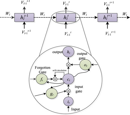
FIGURE 1. LSTM structure diagram.
Where gt is the temporary memory unit, ct is the new memory unit,
The BNN is constructed by integrating the prior distribution over the weight parameters of the LSTM layer in the paper, and its structure is shown in Figure 2. The structure of a Bayesian neural network is similar to that of a traditional deep neural network, which also consists of three layers: input layer, hidden layer, and output layer. However it is different from other types of neural networks in that it has a probability layer, and the weights of the probability layer obey the probability distribution.
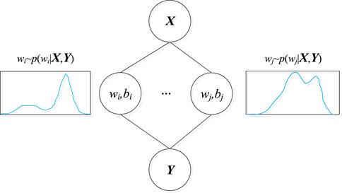
FIGURE 2. Bayesian neural network probability layer structure.
In Figure 2, X is the input of the hidden layer, and Y is the output of the hidden layer; wi and bi are the weight and bias of the ith neuron, respectively, where the weight obeys the probability distribution in the form of p (wi|X,Y).
The unique probability layer of the Bayesian neural network enables the network to express uncertainty, and it has a variety of different output possibilities under specific input. So the Bayesian neural network itself can be regarded as the fusion of infinite sub-networks, similar to the ensemble neural network. However, different from the simple fusion of general neural networks, the sub-networks of Bayesian neural networks are not unrelated to each other. In the actual training process, all sub-networks can be optimized in each round of training. However, in the process of prediction, the final result of prediction can come from several different sub-networks by implementing forward propagation on the same test set several times, so the Bayesian deep network model has a good regularization effect, which can better restrain over-fitting than general neural networks.
Temporal convolutional neural network (TCNN) is designed for sequence modeling tasks and has been widely used in sequence modeling of different data types, including time series prediction (Bai et al., 2018; Chen et al., 2020; Yang et al., 2020). The general architecture of TCNN is shown in Figure 3, which is informed by the CNN architecture and combines autoregressive prediction with long memory. TCNN is a layered architecture, which consists of several convolution hidden layers with the same size as the input layer.
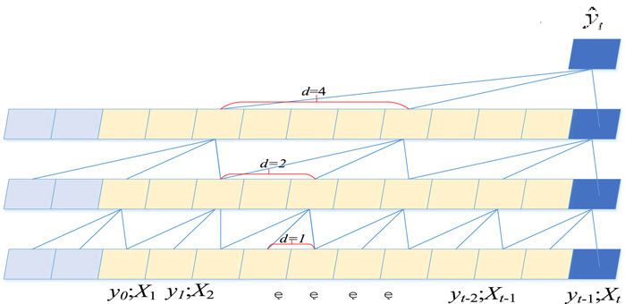
FIGURE 3. TCNN structure.
TCNN includes three parts: causal convolution, dilated convolution, and residual connection. Causal convolution means that the output at time t is only determined by the convolution of the input at time t or earlier in the previous layer, which uses zero padding in the hidden layer to ensure that the hidden layer has the same dimension as the input layer to promote convolution.
Dilated convolution can achieve a larger receptive field to capture long memory. In the dilated convolution operation, the convolution kernels of all layers remain unchanged, but the dilated factor d increases exponentially with the network depth d = 2L, where l is the number of network layers. As shown in Figure 3, Xt is the temporal input variable associated with the predicted output, yt is the temporal prediction output. And d is 1 in the first layer, then increases in each layer, and reaches 4 in the last hidden layer. This pyramid structure and aggregation mechanism effectively increase the receptive field of TCNN, allowing coverage of long input sequences.
TCNN also uses residual connection, as shown in Figure 4. Residual connection helps to overcome the problem of gradient disappearance in multi-layer networks. It has two branches, one of which transforms the input x by a series of stacked layers, including two null causal convolutional layers, and the other is a direct connection of the input x. However, the original input x and the output of the residual block have different widths, and the addition operation cannot be performed. The 1 × 1 convolution layer is used to correct the direct branch to ensure the same width.
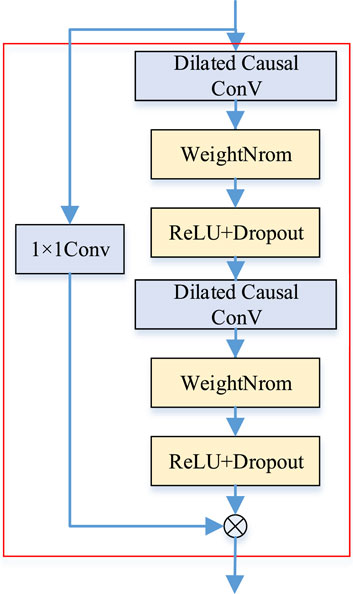
FIGURE 4. Residual connection of TCNN network.
Compared with recurrent architectures such as RNN, LSTM, and GRU, TCNN has the advantages of larger receptive field size, more stable gradient, and stronger parallelism by means of dilated convolution, causal convolution, and residual connection.
In order to fully capture the serial time dependence of wind power historical data and current wind power, this paper adopts TCNN to process the wind power historical time series data, feeding TCNN with the historical power values of the first 24 sampling moments, and feeding the predicted output of TCNN to the BNN-LSTM probabilistic layer.
The Embedding method was originally designed to solve the problem of the sparse matrix of word One-hot representation in natural language processing and the inability to reflect the semantic relationship between words. Paccanaro et al.proposed a word embedding word vector representation method, which can map the original word sparse vector to a low-dimensional dense vector (Paccanaro et al., 2001). Subsequently, the Embedding method has been widely used, and the Embedding method has also become a preprocessing stage of deep learning as a feature engineering (Mikolov et al., 2013). This paper takes the wind power time feature as an entity, performs the Embedding operation on the wind power time, and takes the generated Embedding feature vector as the pre-training vector.
Wind power has the regularity of periodic change with time (such as year, season, etc.). In order to ensure that the constructed wind power prediction network can learn time classification features, such as months in a year, days in a week, days in a month, hours in a day, and minutes in an hour. In this paper, the embedding structure is used to map the discrete features, and the discrete (such as integer years, months, etc.) input is mapped into the geometric vector space. For similar discrete features, they will be embedded into similar vectors, which can well characterize the time periodicity and classification features of wind power, and form the prediction pre-training vector.
The Embedding structure is used to encode each category feature, such as months in 1 year and minutes in 1 hour. These features are then combined and finally connected to a two-layer fully connected layer (FC). The FC layer also adds a residual connection, as shown in Figure 5.
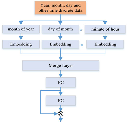
FIGURE 5. Embedding structure of wind power time feature.
Mutual information is a way to measure the degree of information sharing between variables in information theory, which characterizes how well a random variable correlates with information about another random variable (Cao et al., 2012; Feng et al., 2017).
Define the vector X = [x1, x2, … xn], n is the length of X. Normalize X as shown in equation (6).
where X0 is the result of the X-normalization process.
Assuming that B is the group distance of X0, and Ei is the upper and lower limits of the fluctuation interval of X0, the calculation formulas are shown in equations (7) and (8) respectively.
Based on the one-dimensional histogram analysis method, X0 is divided into n fluctuation intervals according to Eq 4, and Xi denotes the i-th fluctuation interval, as shown in Eq 9.
Assuming that p (·) denotes the upper and lower probability density function, the upper and lower bound probability density p (Xi) of each fluctuation interval Xi is:
where ni is the number of data samples of elements in X0 in the fluctuation interval Xi.
The self-information entropy H(Xi) is used to characterize the magnitude of uncertainty in the random fluctuations of X itself, i.e.,
According to Shannon Information Theory, the self-information entropy H(Xi) of a one-dimensional vector is extended to the mutual information I(X;Y), that is:
where Y is a vector different from X, p (Yj) is the upper and lower probability density of the fluctuation interval Yj, and p (XiYj) represents the joint probability density of X0 and Y0 in fluctuation interval Xi and Yj.
I(X;Y) characterizes the degree of information sharing between X and Y, which can be used to measure the correlation between one variable and the other. If vector X and vector Y are independent and unrelated to each other, then vector X will not provide any information to vector Y, and the mutual information between them is zero. on the contrary, if vector X and vector Y are related to each other, then all the information passed between X and Y will be shared, and then the mutual information between them I(X;Y) = 1.
To eliminate the effect of the magnitude, the generalized mutual information I(X;Y) is calculated after normalization to obtain the final MIE correlation coefficient IXY For.
where H(Y) denotes the self-information entropy of the vector Y.
MIE characterizes the statistical properties of the probability distribution between variables, which is always non-negative, i.e., IXY≥0, and is related to the generalized linear correlation coefficient, which can be applied to a wider range. It can better mine the nonlinear correlation between meteorological factors and wind power, and is conducive to the screening of key meteorological features.
Wind power is related to a variety of meteorological factors, such as wind speed, wind direction, temperature, and barometric pressure, but each factor has different degrees of influence on wind power prediction. If all factors are fed into BNN-LSTM, on the one hand, it results in a complex model structure with many parameters and low efficiency, and at the same time, the inclusion of factors that have a low correlation with the wind power is a kind of noise interference to the prediction model, and will bring a negative impact, thus reducing the prediction accuracy of the model. Therefore, a correlation analysis of the wind power dataset is needed to eliminate factors of little value and also to reduce the data dimensionality.
Assuming that each meteorological variable
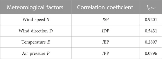
TABLE 1. MIE correlation coefficients of each meteorological factor and wind power.
From Table 1, it can be seen that the MIE correlation coefficients of each meteorological factor with wind power are wind speed, wind direction, temperature and pressure from the largest to the smallest, i.e., wind speed and wind direction have the highest correlation with wind power, which are greater than 0.5. In order to maximize the balance between training accuracy and training efficiency, the top two meteorological factors with high MIE correlation coefficients, wind speed, and wind direction, are finally used as the optimized meteorological input features in this paper.
The improved BNN-LSTM prediction model constructed in this paper includes three components. The TCNN network is utilized to process the wind power historical data and extract the temporal data association features, and then the learned trend feature data is used as one of the BNN-LSTM probabilistic layer input data subsets. The information entropy method is utilized to downscale the wind power related meteorological variables, and the downsized meteorological variables are used as one of the input data subsets of the BNN-LSTM probabilistic layer. Then, the Embedding structure is used to learn the temporal classification features, and the vector encoded by the Embedding structure is used as one of the input data subsets of the BNN-LSTM probability layer, and finally the three subsets are fed into the constructed BNN-LSTM prediction model through fusion, and the model structure is shown in Figure 6.

FIGURE 6. Structure of improved BNN-LSTM wind power prediction model.
The specific steps are as follows.
1) Input data preprocessing and feature engineering. The input features are collected, and the preprocessing and feature extraction of wind power historical data prediction, meteorological data dimension reduction, wind power time discrete feature Embedding are carried out according to the requirements of different input channels.
2) Model training. The data after the preprocessing of the training set is input into the model for training, the Adam method is used to optimize the loss function, and the early termination strategy is used to suppress overfitting.
3) Output of prediction results. The Monte Carlo sampling method is used to predict all the prediction results after several times.
A good prediction error index is helpful for better iterative optimization of the prediction model, and it can also facilitate the comparison between different algorithms. This paper selects the common root mean square error (RMSE), mean absolute error (MAE), mean absolute percentage error (MAPE), and Coefficient of determination (R2) as the point prediction error index, and the specific definitions are as follows.
a) Root mean square error
b) Average absolute error
c) mean absolute percentage error
d) Coefficient of determination
where T is the number of sampling time points. Pi and
For wind power probabilistic prediction, this paper adopts two commonly used probabilistic evaluation methods for wind power probabilistic prediction evaluation. One is the pinball loss score, which can comprehensively indicate reliability and sharpness, and the other is the Winkler score, which can indicate the sharpness and unconditional coverage of the prediction interval.
In this paper, the pinball loss score function used is:
where f(x) are prediction values and y are actual values, and τ∈[0,1]. It can be seen that the pinball loss score function not only penalizes the wrongly classified samples, but also gives an additional penalty to the correctly classified samples; in addition, since the function uses the quantile distance, it is not sensitive to noise, and the data is heavy. Sampling is more stable and does not increase computational cost.
The Winkler Score takes into account the width and coverage of the interval forecast given by the confidence (1-α). At time t, assuming that the confidence (1 − α) × 100% prediction interval [Dt, Ut] corresponds to the true value of Vt, it is defined as:
where δ = Ut− Dt represents the interval width. If the true value is outside the prediction interval, the Winkler score gives a penalty based on α. In the same way, by calculating and summing the Winkler scores of all time points within the prediction time range, the total Winkler score of the prediction results in this interval is obtained. Therefore, a lower Winkler score indicates a better prediction interval.
The dataset used in this paper is from ERCOT Wind power plant data from 2017 to 2019 (Ko et al., 2020), the dataset contains time, meteorological, and wind power data with 1 h interval of data. Of the total dataset, 70%, 20%, and 10% portions are used for the training, testing, and validation sets, respectively. In this paper, we use pytorch1.11 to build the network model, and the GPU model used is GEForce RTX 3060Ti. The BNN-LSTM model was optimized by small-batch gradient descent using the Adam optimizer with a maximum number of 200 iterations and a random search method for hyperparameter optimization selection, which finally determined a learning rate of 0.01 and a batch size of 64. The time series length was searched from {1,6,12,18,24,30,36}, and based on the Winkler score optimization analysis at the 90 % confidence level, the sequence length of 24 is the best, as shown in Figure 7.
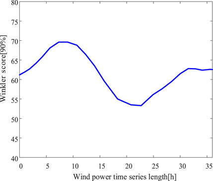
FIGURE 7. Effect of wind power input length on the model.
This paper first establishes a three-layer TCNN wind speed and wind direction prediction model, and predicts the current wind speed and wind direction according to the historical values of wind speed and wind direction. Then, the predicted values of wind speed and wind direction are used as the input of meteorological factors, and based on the method described in Section 2.1, the wind power prediction model is trained in the way of data division in Section 3.1.
After training, 20% of the test set data is fed into the improved BNN-LSTM network for testing, and each prediction point is Monte Carlo sampled 100 times to make a scatter plot of the prediction points and compare the prediction results with those of the CNN without probability layer and BiLSTM methods.
It can be seen from Figure 8, 9 that the trend and size of the predicted value and the actual value of both wind speed and wind direction are basically the same. By using the average absolute error formula summarized in 2.3, the average absolute errors of both are 3.54 m/s and 21.7, respectively, which shows that both are small and the prediction effect is good. Figure 10 shows that the predicted value is close to the actual value, and there is only a large error at individual points.
1) Wind speed forecast
2) Wind direction prediction
3) Wind power forecast
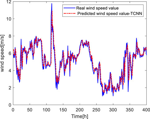
FIGURE 8. Wind speed forecast.
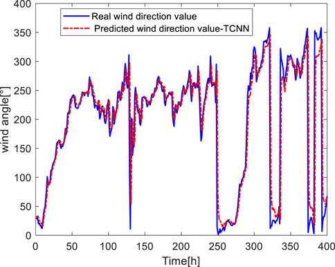
FIGURE 9. Wind direction forecast.
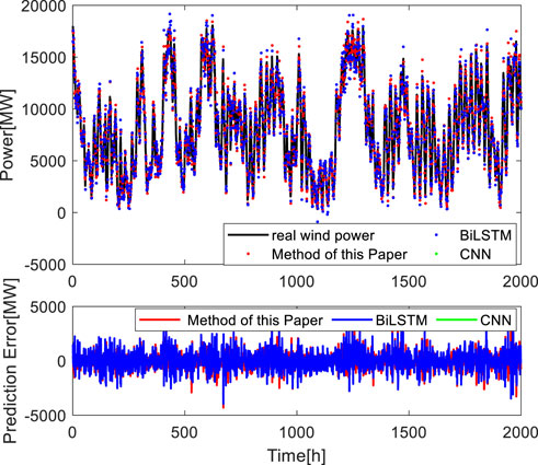
FIGURE 10. Comparison of wind power prediction algorithms.
As can be seen from Figure 10, the predicted value of the algorithm in this paper is close to the actual value, the error value fluctuates around zero, and only a few points have a large error. Table 2 shows the calculation results of RMSE, MAE, MAPE, and R2 indexes of the three algorithms, and the value of each index is the average of each algorithm after 50 times of operation. The results show that the improved BNN-LSTM is dominant in point prediction performance, as indicated by the approximately 13.27%, 13.63%, and 17.42% lower RMSE, MAE, and MAPE respectively and R2 approximately 1.21 % higher, when compared with the method of LSTM. The performance of the improved BNN-LSTM model also dominates when compared with the CNN methods, with approximately 18.48%, 19.78%, 22.81%, and 1.56% improvements in the four evaluation metrics. R2 is a statistical index describing the fitting data of the regression prediction model, which can evaluate the effectiveness and accuracy of the regression prediction model. The better the fitting effect of the prediction model, the higher the R2 evaluation index value. From Table 2, it can be seen that the R2 value of the improved BNN-LSTM is larger and the fitting effect is better. In summary, it can be seen that the prediction model proposed in this paper can better adapt to the actual working conditions of wind turbines and has higher prediction accuracy.
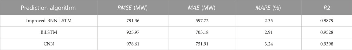
TABLE 2. Comparison of prediction results.
Regarding the computational cost, the times of the training and testing process for all the examined methods are presented in Table 3. It can be seen that the computational complexity of the improved BNN-LSTM is similar to that of the CNN method, and it is faster than the LSTM calculation. The data preprocessing and feature extraction of the proposed method do not bring obvious computational time-consuming increases to the entire network.
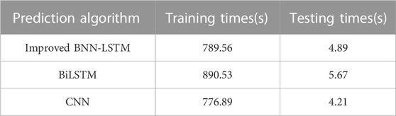
TABLE 3. Comparison of calculation time of different methods.
In order to further test the practical feasibility, superiority, and ability to capture uncertainty of the prediction model described in this paper, the probability prediction of wind power is carried out at 80% and 90% confidence levels, respectively, and the prediction results are shown in Figure 11, 12. At the 80% confidence level, it is compared with the Bayesian neural network and continuous interval prediction method, as shown in Figure 13. Table 4 is the comprehensive probability evaluation index value of different methods. Note that the average of all the Pinball values is calculated to evaluate the overall performance of the probabilistic forecasts for q = 0.01, 0.02,
1) Prediction at 80% confidence level
2) Prediction at 90% confidence level
3) Contrast forecast
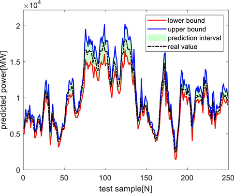
FIGURE 11. Probability prediction of wind power at 80% confidence level.
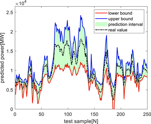
FIGURE 12. Probability prediction of wind power at 90% confidence level.
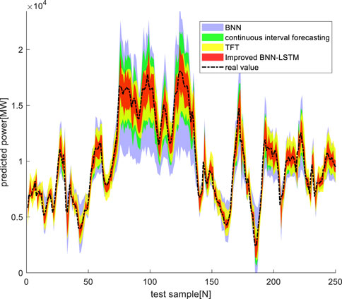
FIGURE 13. Comparison diagram of wind power forecast intervals of different algorithms.
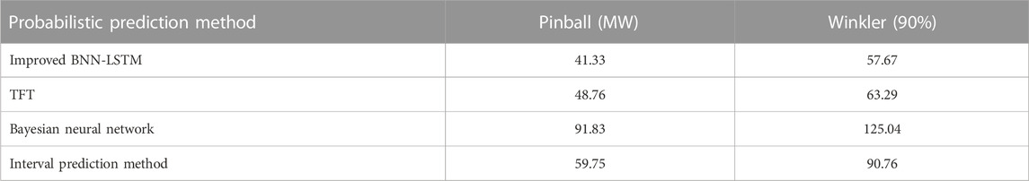
TABLE 4. Comparison of wind power probability prediction performance.
It can be seen from Figure 11, 12 that the improved BNN-LSTM neural network wind power probability prediction model can respond to the power fluctuation in time at different confidence levels, and give the possible power fluctuation range at the next prediction point, with high accuracy.
In general, the probabilistic forecasting performance is evaluated in terms of three primary aspects: reliability, sharpness, and resolution, which have been quantified by the comprehensive evaluation criteria: the pinball loss and the Winkler score. Visually inspecting the results in Figure 13, the probabilistic forecasts generated using the constructed improved BNN-LSTM model present the benefits of a tighter prediction coverage interval, a lower prediction interval that varies over time, and higher unconditional coverage, corresponding to sharpness, resolution, and reliability, respectively (Hong and Fan, 2016).
The pinball index and Winkler index data in Table 4 show that the prediction results obtained by the proposed improved BNN-LSTM have the highest accuracy, followed by Temporal Fusion Transformer (TFT), one of the most advanced temporal prediction networks. The pinball index of the improved BNN-LSTM is 11.3 %, 53.2 %, and 24.4 % smaller than the other three methods, and the Winkler index is 8.2 %, 3.5 % and 34.6 % smaller than the other three methods. The fact that improved BNN-LSTM presents the best predictive capability indicates the significance of capturing both epistemic uncertainty and aleatoric uncertainty.
To further intuitively verify the superiority of the proposed method, based on the comparative simulation experiment in Figure 13, this paper also calculates the prediction interval index of each algorithm, that is, the average interval width in the same prediction period, as shown in Table 5.
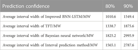
TABLE 5. The index of forecast interval.
It can be seen from Table 5 that the average interval width of the proposed method is smaller under the two confidence levels. Especially when the confidence level reaches 90 %, the average interval width of the proposed method is much smaller than that of the other two traditional methods. Compared with the most advanced time series prediction network TFT, it also has certain advantages, which indicates that the proposed method can predict the wind power probability more accurately and at a lower cost, which verifies the superiority of the proposed method.
Aiming at the problem that wind power uncertainty point prediction cannot predict wind power fluctuation. An improved BNN-LSTM prediction model is constructed based on a Bayesian neural network, combined with the advantages of LSTM in processing time-series data in this paper, and the wind power historical time-series power feature input is optimized by TCNN network first. The correlation calculation of complex meteorological input factors affecting wind power prediction is carried out by the mutual information entropy correlation coefficient method, and the factors with low correlation with wind power are eliminated to reduce the input dimensionality and input noise. The temporal classification features are also extracted by Embedding structure by making full use of the periodic fluctuation feature of wind power prediction in time. Finally, the reduced dimensional meteorological factors, TCNN processed power history time series data, and temporal classification features are used as the final inputs. Through the prediction simulation under 80 % and 90 % confidence levels and the comparison with a Bayesian neural network, continuous interval prediction method, and TFT, it can be seen that this paper has great performance advantages in point prediction evaluation indexes RMSE, MAE, MAPE and R2 and probability prediction evaluation indexes Winkler score and pinball loss score, which can better predict the accuracy and volatility of wind power.
Publicly available datasets were analyzed in this study. This data can be found here: Ko M, Lee K, Kim JK, et al. Deep Concatenated Residual Network With Bidirectional LSTM for One-Hour-Ahead Wind Power Forecasting [J]. IEEE Transactions on Sustainable Energy, 2020, 1(99):1-15.
ZD: Writing–original draft. XZ: Methodology, Writing–review and editing. ZL: Data curation, Writing–review and editing. JY: Investigation, Writing–review and editing. XL: Writing–review and editing. QW: Methodology, Writing–review and editing. BZ: Validation, Writing–review and editing.
The author(s) declare that no financial support was received for the research, authorship, and/or publication of this article.
Author ZL was employed by the Hangzhou Hollysys Automation Co., Ltd. Author JY was employed by the PowerChina Sichuan Electric Power Engineering Co., Ltd.
The remaining authors declare that the research was conducted in the absence of any commercial or financial relationships that could be construed as a potential conflict of interest.
All claims expressed in this article are solely those of the authors and do not necessarily represent those of their affiliated organizations, or those of the publisher, the editors and the reviewers. Any product that may be evaluated in this article, or claim that may be made by its manufacturer, is not guaranteed or endorsed by the publisher.
Alkesaiberi, A., Harrou, F., and Sun, Y. (2022). Efficient wind power prediction using machine learning methods: a comparative study. Energies 15, 2327. doi:10.3390/en15072327
Bai, S., Kolter, J. Z., and Koltun, V. (2018). An empirical evaluation of generic convolutional and recurrent networks for sequence modeling. https://arxiv.org/abs/1803.01271.
Cao, Q., Ewing, B. T., and Thompson, M. A. (2012). Forecasting wind speed with recurrent neural networks. Eur. J. Operational Res. 221 (1), 148–154. doi:10.1016/j.ejor.2012.02.042
Chen, Y., Kang, Y., Chen, Y., and Wang, Z. (2020). Probabilistic forecasting with temporal convolutional neural network. Neurocomputing 399 (1), 491–501. doi:10.1016/j.neucom.2020.03.011
Dong, X., Sun, Y., Pu, T., Wang, X., and Li, Y. (2022). Ultrashort-term wind power probabilistic prediction based on time-series hybrid density network. Power Syst. Autom. 46 (14), 93–100. doi:10.7500/AEPS20211208003
Feng, C., Cui, M., Hodge, B.-M., and Zhang, J. (2017). A data-driven multimodel methodology with deep feature selection for short-term wind forecasting. Appl. Energy 190 (2), 1245–1257. doi:10.1016/j.apenergy.2017.01.043
Feng, S., Guo, J., Fu, H., Guan, Z., and Zhou, W. (2023). Probability density prediction of wind power based on ISSA and GRU quantile regression. New Technol. Electr. Eng. Electr. 42 (10), 55–65. doi:10.12067/ATEEE2203037
Gao, X., Wang, G., Yingjun, G., Jingran, S., and Hexu, S. (2023). Short-term wind power probabilistic prediction based on SSA-VMD-LSTM-NKDE. J. Hebei Univ. Sci. Technol. 44 (04), 323–334. doi:10.7535/hbkd.2023yx0400
Harrou, F., Sun, Y., Dairi, A., Taghezouit, B., and Khadraoui, S. (2023). Editorial: advanced data-driven methods for monitoring solar and wind energy systems. Front. Energy Res. 11, 1147746. doi:10.3389/fenrg.2023.1147746
Hittawe, M. M., Langodan, S., Beya, O., Hoteit, I., and Knio, O. (2022). “Efficient SST prediction in the Red Sea using hybrid deep learning-based approach,” in 2022 IEEE 20th International Conference on Industrial Informatics (INDIN), Perth, Australia, July, 2022. doi:10.1109/INDIN51773.2022.9976090
Hochreiter, S., and Schmidhuber, J. (1997). Long short-term memory. Neural comput., 9 (8-9), 1735–1780. doi:10.1162/neco.1997.9.8.1735
Hong, T., and Fan, S. (2016). Probabilistic electric load forecasting: a tutorial review. Int. J. Forecast. 32 (3), 914–938. doi:10.1016/j.ijforecast.2015.11.011
Ko, M., Lee, K., Kim, J.-K., Hong, C. W., and Hur, K. (2020). Deep concatenated residual network with bidirectional LSTM for one-hour-ahead wind power forecasting. IEEE Trans. Sustain. Energy 1 (99), 1–15. doi:10.1109/TSTE.2020.3043884
Lee, J., Wang, W., Harrou, F., and Sun, Y. (2020). Wind power prediction using ensemble learning-based models. IEEE Access 8, 61517–61527. doi:10.1109/ACCESS.2020.2983234
Li, J., Sang, C., Gan, K., and Pan, Y. (2017). Review of wind power prediction technology. Mod. Electr. Power 34 (03), 1–11. doi:10.19725/j.cnki.1007-2322.2017.03.001
Louka, P., Galanis, G., Siebert, N., Kariniotakis, G., Katsafados, P., Pytharoulis, I., et al. (2018). Improvements in wind speed forecasts for wind power prediction purposes using Kalman filtering. J. Wind Eng. Ind. Aerodyn. 96 (12), 2348–2362. doi:10.1016/j.jweia.2008.03.013
Ma, J., Wang, C., Yang, M., and Lin, Y. (2019). Ultra-short-term probabilistic wind turbine power forecast based on empirical dynamic modeling. IEEE Trans. Sustain. Energy 11 (2), 906–915. doi:10.1109/tste.2019.2912270
Mahmoud, T., Dong, Z. Y., and Ma, J. (2018). An advanced approach for optimal wind power generation prediction intervals by using self-adaptive evolutionary extreme learning machine. Renew. Energy 126 (1), 254–269. doi:10.1016/j.renene.2018.03.035
Mikolov, T., Sutskever, I., Chen, K., Corrado, G., and Dean, J. (2013). Distributed representations of words and phrases and their compositionality (J). Adv. Neural Inf. Process. Syst. 23 (10), 1–9. doi:10.48550/arXiv.1310.4546
Paccanaro, A., and Hinton, G. E. (2001). Learning distribut ed representations of concepts using linear relational embedding [J]. IEEE Trans. Knowl. Data Eng. 13 (2), 232–244. doi:10.1109/69.917563
Su, X., Yu, H., Fu, Y., Tian, S., Li, H., Geng, F., et al. (2023). Offshore wind power probabilistic prediction based on DALSTM and joint quantile loss. China Electr. Power 57 (11), 1–10. doi:10.11930/j.issn.1004-9649.202212011
Sun, R., Zhang, T., He, Q., and Xu, H. (2021). Review of key technologies and applications of wind power forecasting. High. Volt. Technol. 47 (04), 1129–1143. doi:10.13336/j.1003-6520.hve.20201780
Wang, H., Wang, G., Li, G., Peng, J., and Liu, Y. (2016). Deep belief network based deterministic and probabilistic wind speed forecasting approach. Appl. Energy 182, 80–93. doi:10.1016/j.apenergy.2016.08.108
Wang, S., Sun, Y., Hou, D., Zhou, Y., and Zhang, W. (2023). Ultra-short-term adaptive probabilistic prediction of wind power based on multi-window wide kernel density estimation. High. Volt. Technol. 50 (1), 1–10. doi:10.13336/j.1003-6520.hve.20230170
Yang, L., Koprinska, I., and Rana, M. (2020). “Temporal convolutional neural networks for solar power forecasting,” in 2020 International Joint Conference on Neural Networks (IJCNN), Glasgow, UK, July, 2020.
Yu, H., Lu, J., Zeng, Y., Duan, P., Liu, J., and Gou, X. (2019). Nonlinear combination forecasting of wind power based on different optimization criteria and generalized regression neural network. High. Volt. Technol. 45 (03), 1002–1008. doi:10.13336/j.1003-6520.hve.20190226042
Zhang, J., Hua, Y., Song, T., Wang, , Xue, Z., Ma, R., et al. (2022). Improving bayesian neural networks by adversarial sampling. Proc. AAAI Conf. Artif. Intell. 36 (9), 10110–10117. doi:10.1609/aaai.v36i9.21250
Zheng, P., Yu, L., Hou, S., and Wang, C. (2020). Multi-step wind power prediction based on Kalman filter correction. Therm. Power Eng. 35 (04), 235–241. doi:10.16146/j.cnki.rndlgc.2020.04.032
Keywords: Bayesian neural network, BNN-LSTM, temporal convolutional neural network, wind power, mutual information entropy, dimensionality reduction, probabilistic prediction
Citation: Deng Z, Zhang X, Li Z, Yang J, Lv X, Wu Q and Zhu B (2024) Probabilistic prediction of wind power based on improved Bayesian neural network. Front. Energy Res. 11:1309778. doi: 10.3389/fenrg.2023.1309778
Received: 08 October 2023; Accepted: 06 December 2023;
Published: 03 January 2024.
Edited by:
Fouzi Harrou, King Abdullah University of Science and Technology, Saudi ArabiaReviewed by:
Mazen Hittawe, King Abdullah University of Science and Technology, Saudi ArabiaCopyright © 2024 Deng, Zhang, Li, Yang, Lv, Wu and Zhu. This is an open-access article distributed under the terms of the Creative Commons Attribution License (CC BY). The use, distribution or reproduction in other forums is permitted, provided the original author(s) and the copyright owner(s) are credited and that the original publication in this journal is cited, in accordance with accepted academic practice. No use, distribution or reproduction is permitted which does not comply with these terms.
*Correspondence: Zhiguang Deng, ZHpnNzQwMDYxM0AxNjMuY29t
Disclaimer: All claims expressed in this article are solely those of the authors and do not necessarily represent those of their affiliated organizations, or those of the publisher, the editors and the reviewers. Any product that may be evaluated in this article or claim that may be made by its manufacturer is not guaranteed or endorsed by the publisher.
Research integrity at Frontiers
Learn more about the work of our research integrity team to safeguard the quality of each article we publish.