 Kai Zhou
 Hao Han
 Lingxiao Jiao
- State Grid Hubei Extra High Voltage Company, Wuhan, Hubei, China
The wind turbine power curve model is critical to a wind turbine’s power prediction and performance analysis. However, abnormal data in the training set decrease the prediction accuracy of trained models. This paper proposes a sample average approach-based method to construct an interval model of a wind turbine, which increases robustness against abnormal data and further improves the model accuracy. We compare our proposed methods with the traditional neural network-based and Bayesian neural network-based models in experimental data-based validations. Our model shows better performance in both accuracy and computational time.
1 Introduction
Wind power has become a significant renewable power source of global energy systems (Gilbert et al., 2020). To ensure operation safety and high efficiency, it is critical to monitor the operation conditions of wind turbines to predict wind power output and detect potential faults (Wang and Liu, 2021). The Supervisory Control and Data Acquisition (SCADA) system provides wind turbine data, for example, wind speed and power, for establishing models for wind turbine power prediction and fault detection (Y. Wang et al., 2019). A significant proportion of the SCADA data is abnormal due to communication failures, maintenance, and other reasons (Morrison et al., 2022). A model trained by a dataset with abnormal data is biased from a real model and suffers from reduced accuracy (Ye et al., 2021). It is necessary to consider the data cleaning-based method to obtain a model with improved robustness against abnormal data.
Prior results of the data cleaning method were based on clustering algorithms (Zheng et al., 2015; 2010; Yesilbudak, 2016). In clustering algorithm-based methods, k-means, manifold spectral clustering, and other algorithms are applied to separate the wind power curve into partitions and then identify the outliers based on distances to the cluster centers. An alternative method is to determine the upper and lower boundaries of the wind power curve by boundary models. For example, Shen et al. (2019) used change point and quantile to estimate a contour for normal data. However, the aforementioned methods fail to identify the outliers when there are many cluster centers. The setting of the algorithm parameters, for example, cluster number in the clustering algorithm-based method, is also unexplainable. These reasons make the clustering algorithm-based and existing boundary methods suffer from issues of misidentification.
Normal distribution model-based methods, proposed to overcome issues of misidentification, use the normal distribution to fit the power data’s distribution and then calculate the probability contours. Data with low probability are regarded as abnormal data. Ouyang et al. (2017) calculated mean and standard deviation values based on exponential smoothing. Stephen et al. (2011) used bivariate joint distribution to fit the wind power data’s distribution.
However, the aforementioned existing methods for abnormal detection toward improving the model accuracy have the following disadvantages:
• Many real outliers, especially those near the normal region, cannot be recognized.
• There are too many hyperparameters to be set. The performance highly depends on the hyperparameters, while the function of each hyperparameter is unexplainable.
• To ensure performance, the prior information on the normal points should be available, which is not practical in general cases.
Another practical way to quantify uncertainty is to directly use a confidence interval-aware model, known as the interval predictor model (Campi et al., 2009; Garattia et al., 2019). The scenario approach presented by Calafiore and Campi (2006); Campi and Garatti (2019); and (2011); Campi et al. (2015) can be used to establish the interval predictor model. However, the scenario approach cannot give an exact confidence bound since a small number of samples will give a bound with high risk, and a large number of samples will give a conservative bound. Luedtke and Ahmed (2008) proposed a sample average approach to obtain an approximate solution that exactly converges to the original as the sample number increases. In this paper, we propose the sample average approach-based interval models and extend them into extreme learning machines to provide a fast algorithm for training neural networks that can exactly give the desired confidence interval. The proposed interval model solves the abnormal detection and wind power curve regression problems together in a direct way. We implement experimental data-based validation to compare the proposed methods with several existing methods.
The rest of this paper is organized in the following way: Section 2 briefly introduces the wind power curve and then gives a formal problem statement. In Section 3, extreme learning machine and the theory of sample average approach for chance-constrained optimization are briefly reviewed; Section 4 presents the proposed interval models combining the extreme learning machine and sample average approach; and Section 5 presents the results and discussions of experimental data-based validation. Finally, Section 6 concludes the paper.
2 Problem description
As shown in Figure 1, a wind turbine power curve has the following three critical points, namely, A, B, and C, which divide the wind turbine power curve into four segments (Marvuglia and Messineo, 2012; Shokrzadeh et al., 2014). Point A is the cut-in wind speed from where the wind turbine starts to output the power. Point B represents the rated power before which the output power increases as the wind speed increases. Point C is the cut-out speed from where the output wind power decreases even with the increased wind speed.
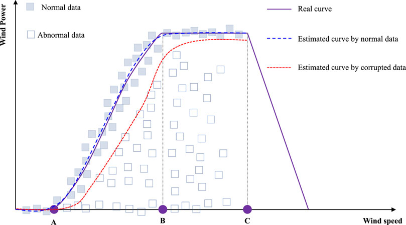
FIGURE 1. Brief illustration of the wind turbine power curve and estimation biases using abnormal data.
The segment between points B and C gives the rated level of the wind power output. The segment between points A and B shows a non-linear correlation between wind speed and power. Let v be the wind speed and P be the wind power. The non-linear correlation can be described approximately by the following equation:
where
A dataset obtained by the SCADA system can be defined by the following equation:
where N is the number of the data samples. As shown in Figure 1, the SCADA system’s data have normal and abnormal data. In other words,
Therefore, it is necessary to investigate a robust power curve estimation method for the abnormal data. In this paper, we address the following problem.
Here, the set
• data cleaning problem to obtain a cleaned data
• regression problem described by (3).
3 Preliminaries
This section briefly reviews the extreme learning machine and sample average approach as a preparation for introducing our proposed interval models.
3.1 Extreme learning machine
Extreme learning machine is a fast algorithm to train a single-layer neural network (Huang et al., 2006). A single-layer neural network has an input layer, a hidden layer, and an output layer. Let a positive integer L be the number of neurons. The hidden layer can be defined as a vector function by the following expression:
Each hi(x), i = 1, …, L is a neuron. Often, we choose the neuron as follows:
where ai, bi are the hyperparameters in the i − th neuron. The neuron can be a sigmoid function or a Gaussian function, etc. Let
be the coefficient of the output layer. Then, we can write the single-layer network as follows:
As a summary, the parameters that need to be trained are coefficient vector β and hyperparameters
The algorithm of the extreme learning machine is summarized as follows:
• randomly generate hyperparameters
• estimate β by solving
which gives the solution as
where
and YN is defined as
Theorem 2.2 of Huang et al. (2006) provides the universal approximation property of an extreme learning machine-based single neural network regarding a dataset
Lemma 1. For any given small ɛ and activation function G(⋅) which is infinitely differentiable in any interval, there exists
Lemma 1 shows that we could use a single-layer neural network to approximate the wind power curve.
3.2 Sample average approach
Chance-constrained optimization seeks to optimize an objective under a stochastic constraint (Campi et al., 2015; Shen et al., 2020; 2021), which is written as follows:
where
The sample-based approximation is a practical way to solve chance-constrained optimization. This paper adopts the sample average approach presented by Luedtke and Ahmed (2008). In the sample average approach, samples are extracted from the sample space Ξ, and then, an approximate problem of the original chance-constrained optimization is established. Let (ξ(1), …, ξ(N)) be an independent Monte Carlo sample set of the random variable ξ. After choosing
where
where Λη(⋅) is defined by the following equation:
Let
The following assumption on G(⋅) holds throughout this paper.
Assumption 1. There exists L > 0 such that
Assumption 1 is reasonable since we could choose an activation function that makes the neural networks satisfy it and also preserve the universal approximation.
The uniform convergence of
Lemma 2. Suppose that Assumption 1 holds as N → ∞, γ → 0, and ϵ → α,
Lemma 2 shows that the approximate problem’s solution converges to one in the solution set of the original problem if the number of samples increases to infinite. In addition, for a certain bounded value, we could use a large enough sample number to ensure that the approximate problem’s solution is within that bound.
4 Proposed method
This section presents the proposed extreme learning machine with a confidence region. The convergence analysis is given. In addition, the proposed algorithm is presented.
4.1 Extreme learning machine with a confidence region
The previous extreme learning machine gives a single prediction value for a given input. In this paper, we investigate a computation method to give a confidence region for a given input with the center of the confidence region as the estimation of the curve and the normal data located in the confidence region with high probability. In this way, we can solve problem (3). The concept of the extreme learning machine with the confidence region is illustrated in Figure 2
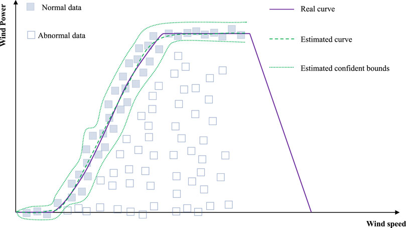
FIGURE 2. Basic concept of the extreme learning machine with a confidence region.
We want to establish an interval model to give a power curve’s interval for any given wind speed and require the correct wind power prediction to be within the interval at a given probability. This interval should be the smallest since a large interval has the issue of being too conservative. An interval model based on a single-layer neural network can be defined by the following equation:
Let
be the parameter vector that specifies the interval. We have a set of θ as
In this paper, we use a ball set for
With
Then, the problem of solving the extreme learning machine with a confidence region is written as follows:
Here, η is a positive number. By using the extreme learning machine algorithm (Lemma 1), we can obtain
Let z and
be the optimal objective value of problem (20) and
be the optimal solution set. Let
4.2 Sample-based approximation and proposed algorithm
Due to chance constraints, problem (20) is not intractable. With the sample set
Here,
Theorem 1. As N → ∞ and ɛ′ → ɛ,
Proof. Theorem 1 can be proved by directly applying Lemma 2 since problem (20) satisfies Assumption 1.
The proposed algorithm of the extreme learning machine with a confidence region is presented as follows.
Algorithm 1.Proposed algorithm of the extreme learning machine with a confidence region.
Inputs: Dataset
1: Solve Problem (23) to obtain
2: Abnormal data detection
3: Estimated curve
Output:
Notice that (25) gives the estimated curve. The confidence bound (upper and lower bounds) can be given using the interval obtained by solving Problem (23).
5 Experimental data-based validation
This section presents the results of experimental data-based validations. First, the experimental dataset is introduced. Then, the results given by the proposed method and several existing methods are compared.
5.1 Experimental data and settings
Figure 3 plots the data used in this validation. The dataset was collected from a wind farm in Hubei, China. Figure 3A shows all data, including abnormal data and normal data. Specialists were approached to give labels on the data set. The data with labels are plotted in Figure 3B.
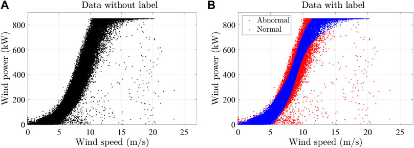
FIGURE 3. Experimental dataset: (A) data without labels and (B) data with labels.
In this paper, we compare the performance of the following methods:
• TrueELM: extreme learning machine using normal data;
• SSELM: the proposed extreme learning machine combined with the sample average approach;
• ELM: extreme learning machine without data cleaning;
• BELM: Bayesian extreme learning machine proposed by Soria-Olivas et al. (2011);
• SNN: Neural network trained by the scenario approach presented by Sadeghi et al. (2019).
In BELM, the parameter β is assumed to obey some predefined distribution. First, a prior distribution is set. With new data, the prior distribution is adjusted to a posterior distribution so that the data have maximum likelihood. Then, the corresponding output will also have a conditional probability, from which the confidence interval can be calculated. In addition, SNN can be regarded as a special case of SSELM with ɛ′ = 0.
We evaluate the mean square error (MSE) and mean absolute error (MAE) regarding the normal data in the evaluations.
5.2 Results and discussions
Figure 4 gives the examples of boundaries estimated by SSELM, BELM, and SNN. For each method, 10,000 samples are used. For SSELM, the probability threshold is set as 0.09. Each method also gives a corresponding center point of the confidence region. The abnormal data detection performance of different methods is summarized in Table 1. SSELM shows a better performance than other methods. The reason that SNN shows a poor performance is that it includes more abnormal data since it essentially gives a completely robust interval.
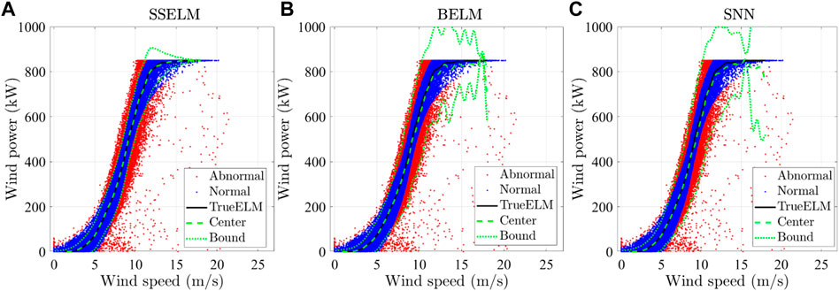
FIGURE 4. Examples of boundaries: (A) SSELM, (B) BELM, and (C) SNN.

TABLE 1. Abnormal data detection accuracy (%) of different methods.
The results of wind power predictions on a text set are plotted in Figure 5. Note that the proposed method, SSELM, gives a prediction that concentrates around the real value with a shorter distance. More comprehensive results of error statistics are summarized in Table 2, which shows that the proposed method, SSELM, performs very close to the results the method gave using normal data. This shows the effectiveness of the proposed method. The proposed method increases the robustness of the regression against the abnormal data since it can clean the abnormal data effectively and thus increases the accuracy of regression.
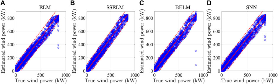
FIGURE 5. Results of wind power predictions on a test set by different methods: (A) ELM, (B) SSELM, (C) BELM, and (D) SNN.

TABLE 2. Error statistics of different methods.
6 Conclusion
This paper proposes an interval model of wind turbine power curves to improve the accuracy of wind power prediction. The interval model combines an extreme learning machine and the sample average approach. Thus, the proposed interval model can give a confidence region and center point of the wind power prediction for a given wind speed. The confidence region can be used for abnormal data detection, and the center point can be used as the estimation of the wind turbine power curve point. Experimental data-based validations have been conducted to compare the proposed method with several existing methods. The results show that the proposed method improves the accuracy of both abnormal detection and wind power curve estimation.
Data availability statement
The original contributions presented in the study are included in the article/Supplementary Material, further inquiries can be directed to the corresponding author.
Author contributions
KZ: conceptualization, methodology, project administration, writing–original manuscript, and writing–review and editing. HH: data curation, formal analysis, software, supervision, validation, and writing–review and editing. JL: data curation, investigation, methodology, and writing–review and editing. YW: investigation, validation, visualization, and writing–review and editing. WT: data curation, formal analysis, resources, and writing–review and editing. FH: formal analysis, supervision, validation, and writing–review and editing. YL: methodology and writing–review and editing. RB: data curation, formal analysis, resources, and writing–review and editing. HZ: data curation, investigation, validation, and writing–review and editing. LJ: methodology, supervision, and writing–review and editing.
Funding
This work was supported by the Science and Technology Project of State Grid Hubei Electric Power Company (52152020003K).
Conflict of interest
Authors KZ, HH, JL, YW, WT, FH, YL, RB, HZ, and LJ were employed by State Grid Hubei Extra High Voltage Company.
Publisher’s note
All claims expressed in this article are solely those of the authors and do not necessarily represent those of their affiliated organizations, or those of the publisher, the editors, and the reviewers. Any product that may be evaluated in this article, or claim that may be made by its manufacturer, is not guaranteed or endorsed by the publisher.
References
Calafiore, G., and Campi, M. C. (2006). The scenario approach to robust control design. IEEE Trans. Autom. Control 51, 742–753. doi:10.1109/tac.2006.875041
Campi, M., Garatti, S., and Ramponi, F. (2015). A general scenario theory for nonconvex optimization and decision making. IEEE Trans. Automatic Control 63, 4067–4078. doi:10.1109/tac.2018.2808446
Campi, M. C., Calafiore, G., and Garatti, S. (2009). Interval predictor models: identification and reliability. Automatica 45, 382–392. doi:10.1016/j.automatica.2008.09.004
Campi, M. C., and Garatti, S. (2011). A sampling-and-discarding approach to chance-constrained optimization: feasibility and optimality. J. Optim. Theory Appl. 148, 257–280. doi:10.1007/s10957-010-9754-6
Campi, M. C., and Garatti, S. (2019). Introduction to the scenario approach. Philadelphia: MOS-SIAM Series on Optimization.
Garattia, S., Campib, M., and Care, A. (2019). On a class of interval predictor models with universal reliability. Automatica 110, 108542. doi:10.1016/j.automatica.2019.108542
Gilbert, C., Browell, J., and McMillan, D. (2020). Leveraging turbine-level data for improved probabilistic wind power forecasting. IEEE Trans. Sustain. Energy 11, 1152–1160. doi:10.1109/tste.2019.2920085
Huang, G., Zhu, Q. Y., and Siew, C. K. (2006). Extreme learning machine: theory and applications. Neurocomputing 70, 489–501. doi:10.1016/j.neucom.2005.12.126
Luedtke, J., and Ahmed, S. (2008). A sample approximation approach for optimization with probabilistic constraints. SIAM J. Optim. 19, 674–699. doi:10.1137/070702928
Marvuglia, A., and Messineo, A. (2012). Monitoring of wind farms’ power curves using machine learning techniques. Appl. Energy 98, 574–583. doi:10.1016/j.apenergy.2012.04.037
Morrison, R., Liu, X., and Lin, Z. (2022). Anomaly detection in wind turbine scada data for power curve cleaning. Renew. Energy 184, 473–486. doi:10.1016/j.renene.2021.11.118
Ouyang, T., Kusiak, A., and He, Y. (2017). Modeling wind-turbine power curve: a data partitioning and mining approach. Renew. Energy 102, 1–8. doi:10.1016/j.renene.2016.10.032
Sadeghi, J., Angelis, M., and Patelli, E. (2019). Efficient training of interval neural networks for imprecise training data. Neural Netw. 118, 338–351. doi:10.1016/j.neunet.2019.07.005
Shen, X., Fu, X., and Zhou, C. (2019). A combined algorithm for cleaning abnormal data of wind turbine power curve based on change point grouping algorithm and quartile algorithm. IEEE Trans. Sustain. Energy 10, 46–54. doi:10.1109/tste.2018.2822682
Shen, X., Ouyang, T., Yang, N., and Zhuang, J. (2021). Sample-based neural approximation approach for probabilistic constrained programs. IEEE Trans. Neural Netw. Learn. Syst. 34, 1058–1065. doi:10.1109/tnnls.2021.3102323
Shen, X., Ouyang, T., Zhang, Y., and Zhang, X. (2020). Computing probabilistic bounds on state trajectories for uncertain systems. IEEE Trans. Emerg. Top. Comput. Intell. early access 7, 285–290. doi:10.1109/TETCI.2020.3019040
Shokrzadeh, S., Jafari Jozani, M., and Bibeau, E. (2014). Wind turbine power curve modeling using advanced parametric and nonparametric methods. IEEE Trans. Sustain. Energy 5, 1262–1269. doi:10.1109/tste.2014.2345059
Soria-Olivas, E., Gomez-Sanchis, J., Martin, J. D., Vila-Frances, J., Martinez, M., Magdalena, J. R., et al. (2011). Belm: Bayesian extreme learning machine. IEEE Trans. Neural Netw. 22, 505–509. doi:10.1109/tnn.2010.2103956
Stephen, B., Galloway, S. J., McMillan, D., Hill, D. C., and Infield, D. G. (2011). A copula model of wind turbine performance. IEEE Trans. Power Syst. 26, 965–966. doi:10.1109/tpwrs.2010.2073550
Wang, Y., Srinivasan, D., and Wang, Z. (2019). Wind power curve modeling and wind power forecasting with inconsistent data. IEEE Trans. Sustain. Energy 10, 16–25. doi:10.1109/tste.2018.2820198
Wang, Z., and Liu, C. (2021). Wind turbine condition monitoring based on a novel multivariate state estimation technique. Measurement 168, 108388. doi:10.1016/j.measurement.2020.108388
Ye, Z., Chen, Y., and Zheng, H. (2021). Understand the effect of bias in deep anomaly detection. Proc. 30th Int. Conf. Artif. Intell., 3314–3320. doi:10.48550/arXiv.2105.07346
Yesilbudak, M. (2016). “Partitional clustering-based outlier detection for power curve optimization of wind turbines,” in Proc. IEEE Int. Conf. Renewable Energy Res. Appl, Birmingham, UK, 20-23 November 2016, 1080–1084.
Zheng, L., Hu, W., and Min, Y. (2010). Short-horizon prediction of wind power: a data-driven approach. IEEE Trans. Energy Convers 25, 1112–1122. doi:10.1109/tec.2010.2043436
Keywords: abnormal detection, data cleaning, wind power prediction, prediction accuracy, stochastic optimization
Citation: Zhou K, Han H, Li J, Wang Y, Tang W, Han F, Li Y, Bi R, Zhao H and Jiao L (2023) Interval model of a wind turbine power curve. Front. Energy Res. 11:1305612. doi: 10.3389/fenrg.2023.1305612
Received: 02 October 2023; Accepted: 31 October 2023;
Published: 24 November 2023.
Edited by:
Xun Shen, Osaka University, JapanReviewed by:
Hardeep Singh, University of Windsor, CanadaShuang Zhao, Hefei University of Technology, China
Yikui Liu, Stevens Institute of Technology, United States
Copyright © 2023 Zhou, Han, Li, Wang, Tang, Han, Li, Bi, Zhao and Jiao. This is an open-access article distributed under the terms of the Creative Commons Attribution License (CC BY). The use, distribution or reproduction in other forums is permitted, provided the original author(s) and the copyright owner(s) are credited and that the original publication in this journal is cited, in accordance with accepted academic practice. No use, distribution or reproduction is permitted which does not comply with these terms.
*Correspondence: Lingxiao Jiao, MTA2MjQ5NTAxN0BxcS5jb20=