Planning model for rural distribution networks with integrated energy stations via robust optimization method

With the modernization and intelligent development of agriculture, the energy demand in rural areas continues to increase, which leads to an increased operational burden on the existing rural distribution network. Integrated energy stations (IESs), in rural areas, use renewable energy sources such as biogas, wind power, and photovoltaic as energy inputs, which can fully improve energy efficiency and help reduce the operating load and peak valley difference of rural distribution networks. In this paper, a multistage planning model is proposed for rural distribution networks with IESs based on the robust optimization method. Firstly, a rural distribution network operation framework with IESs is proposed, and a mathematical model of rural IESs is built based on the energy hub (EH). Then, the multistage robust planning model of rural distribution net-works with IESs is developed and typical scenarios of stochastic source and load are generated based on improved k-means. An iterative solution method for a two-stage robust optimization method is proposed based on the nested column constraint generation (NC&CG) algorithm. Finally, the effectiveness of the presented model and solution approach is assessed through case studies on a modified IEEE 33-node distribution network and a real 152-node distribution network.

1 Introduction

With the continuous construction of modern agriculture in rural areas, the demand for electricity among residents has increased rapidly (Han, Zhang and Li, 2022). The air conditioning load is one of the primary causes of the constant rise in power consumption. Additionally, because of the air-conditioning load’s focused energy demand, the power grid’s peak and valley differences are becoming more significant (International Energy Agency, 2015). In this context, the development and construction of the distribution network framework are facing new challenges. Therefore, it is crucial to help rural distribution network planning and construction through the multi-energy complementary advantages of integrated energy stations.

In response to the increasing load growth, conventional distribution network planning usually determines what type of lines to build, the capacity and location of transformer substation (TS) based on the peak value of load forecast. As proposed in reference (Heidari and Fotuhi-Firuzabad, 2019), a distribution network planning model suitable for multiple power sources is proposed. The objective of minimizing the investment cost and operation cost is to determine the conventional lines of the distribution network. Ref (Dong et al., 2022). considers the correlation and timing of the outputs of distributed power sources in the distribution network, and conducts collaborative planning between the distribution network structure and distributed power sources, taking into account load growth. Ref (Li, Wang and Xia, 2017). proposes an active distribution network collaborative planning method considering energy storage devices and distributed power sources. Although the implementation of these planning approaches has the potential to enhance the operational adaptability of the distribution network, their practical application is hindered by the issue of substantial investment expenses. Additionally, it is worth noting that the majority of the aforementioned research focuses on urban distribution network planning, leaving the exploration of rural distribution networks in its nascent stage.

The concept of IES has been pioneered in Europe and the United States in order to address the challenges posed by the energy transition. By coordinating and integrating various energy systems, such as cooling, electricity, heat, and gas, through collaborative planning and synergistic operations, the aim is to overcome the current limitations of separate operations and enhance the overall efficiency and utilization of energy systems (Wu et al., 2016). Ref (Wu et al., 2017). utilizes the time-delay characteristics of heat networks and the thermal inertia of buildings in different regions to promote the optimal operation of multi-region electricity-heat. A multistage planning approach for IES for converged distribution networks is proposed in (Li et al., 2022a) to minimize the total costs. Ref (Ge, Liu and Ge, 2018). considered the participation of electricity, heat, and cold storage in interaction in IES planning, and compared the differences in planning capacity among the three under different objectives such as economy and energy conversion efficiency. In contrast to power storage devices, cold and heat storage devices have achieved a higher level of development and are more cost-effective, rendering them more viable for the implementation of energy storage in rural areas. However, most of the above references focuses on IES as the main body and distribution networks and other energy networks as the component elements to achieve the overall system planning. Less attention has been paid to the application value of IES as an energy coupling node for distribution network planning.

IES also faces uncertainty in the operation of multi-energy loads and renewable energy output. The different methods of handling random variable prediction errors, it is mainly divided into scenario method (Li et al., 2022b), chance-constrained programming (Huo et al., 2021), robust optimization (Gan et al., 2021), etc. A scenario-generation based approach for integrated regional energy expansion planning was proposed in (Lei et al., 2020). The method considers the temporal, autocorrelation and inter-correlation properties of renewable energy sources and multi-energy loads. Based on the spatial and temporal correlation of PV output, ref (Koutsoukis and Georgilakis, 2019). established a multi-objective distributed power grid-connected planning model by utilizing opportunity constraint planning, taking into account the total cost of PV and the cost of grid operation. A robust return on investment oriented optimal allocation method is proposed in (Jiang et al., 2020) to address the uncertainty of wind power output and multi-energy load. In which, the planning method based on robust optimization fully considers the possible worst scenarios of random variables in the planning stage, which can ensure the robustness of the planning scheme and has a wide range of application scenarios. The typical scenarios in existing scenario methods and the basic scenarios in robust planning methods are usually obtained by clustering algorithms such as k-means. However, the clustering number of existing k-means is artificially given and has a certain degree of subjectivity.

In summary, existing research on urban distribution network planning is relatively rich, but rural distribution network planning is still in its early stages. There exist notable disparities in terms of source and load characteristics between rural and urban regions, and existing plans for urban distribution networks do not apply to rural areas. In addition, it is also necessary to conduct research on distribution network planning with the distribution network as the main body and IES as the means of distribution network regulation. Therefore, the main contributions of this article are as shown below.

1) A multistage planning model for rural distribution network with integrated energy stations is proposed. The primary focus of the model is the distribution network, with the IES serving as a regulatory entity to address the increasing demand in rural areas and mitigate fluctuations in load levels. The model implements a multistage rolling plan that encompasses various aspects such as distribution line management, TS expansion, and investment and construction of the IES.

2) Utilizing an enhanced k-means clustering algorithm to derive multiple representative daily load patterns from projected annual load data. The method aims to improve clustering efficiency by calculating clustering performance evaluation indicators to ascertain the most suitable number of clusters, thereby solving the problem of traditional k-means algorithms being unable to determine the optimal number of clusters.

The subsequent organization of this article is outlined as follows. Section 2 provides an introduction to the operational framework of rural distribution networks incorporating integrated energy stations. In section 3, a multistage robust planning model for rural distribution networks with integrated energy stations is proposed. Section 4 elaborates on the solution methods for robust programming models. Section 5 presents the simulation results. Section 6 summarizes the entire text.

2 Operational framework for rural distribution networks with IES

2.1 Structure of the rural distribution network with IES

In this paper, we consider the current situation that in the development of biogas in rural, biogas projects with a variety of feedstock substrates are gradually formed, and the gas production capacity increases year after year (Yan et al., 2021). Therefore, biogas is used as the gas input for IES in the IES configuration. In addition, the main focus of this article is on the planning method of rural distribution networks. Therefore, non-distribution network structures such as gas networks have been weakened and set to have gas source points at the construction site of IES to meet the gas demand of IES.

The structure of the rural distribution network with IES is depicted in Figure 1. The voltage level of the rural distribution network shown in Figure 1 is 10kV, with IES built on some network nodes. The Integrated Energy System comprises a diverse range of equipment, encompassing combined heat and power (CHP), gas boilers (GB), electric refrigeration (ER), absorption refrigeration (AR), cold energy storage (CES), and thermal energy storage (TES). The specific direction of energy flow is shown in Figure 1, where the CHP consumes biogas to generate electricity and purchases electricity from the distribution network to transmit to the load and ER. The thermal load and AR are sup-plied by TES heat release, CHP, and GB consumption of biogas, while the excess thermal energy is stored in TES. The cooling load is jointly supplied by CES cooling, ER, and AR cooling, and the excess cold energy is stored in CES.

FIGURE 1

FIGURE 1. Energy flow structure of rural distribution network with integrated energy stations.

2.2 Modeling of rural integrated energy stations based on EH

After the IES is connected to the rural distribution system, there are multiple energy coupling relationships within the system. Considering the energy supply perspective, the rural integrated energy station (RIES) generally includes energy supply means such as TS, GB, CHP, and ER. The EH-based model, as depicted in Figure 2, is commonly employed to describe the multi-energy attributes of RIES (Moazeni, Miragha and Defourny, 2018).

FIGURE 2

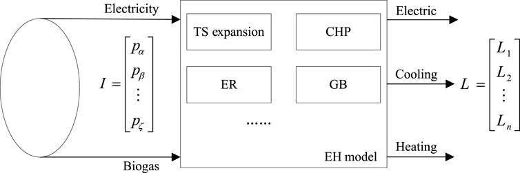
FIGURE 2. Typical EH-based RIES.

EH takes into account various forms of energy input and output, and represents its energy conversion relationship through a set of linear equations.

$L=\left[\begin{array}{c}{L}_1\\ L_2\\ ⋮\\ L_n\end{array}\right]=\left[\begin{array}{cccc}{\mathfrak{R}}_{\alpha ,1}& {\mathfrak{R}}_{\beta ,1}& \cdots & {\mathfrak{R}}_{\zeta ,1}\\ {\mathfrak{R}}_{\alpha ,2}& {\mathfrak{R}}_{\beta ,2}& \cdots & {\mathfrak{R}}_{\zeta ,2}\\ ⋮& ⋮& \ddots & ⋮\\ {\mathfrak{R}}_{\alpha ,n}& {\mathfrak{R}}_{\beta ,n}& \cdots & {\mathfrak{R}}_{\zeta ,n}\end{array}\right]\left[\begin{array}{c}{p}_{\alpha }\\ p_{\beta }\\ ⋮\\ p_{\zeta }\end{array}\right]=UI(1)$

where $L={\left[L_1,L_2,\cdots ,L_n\right]}^T$ represents the output part of EH, and subscript $\mathrm{1,2},\cdots ,n$ represents different forms of energy demand on the load side, such as electrical load, heating load, cooling load, etc.; $I={\left[p_{\alpha },p_{\beta },\cdots ,p_{\zeta }\right]}^T$ represents the input part of EH, where subscript $\alpha ,\beta ,\cdots ,\zeta$ represents different types of energy input forms, such as electricity, heat, biogas, etc.; $U$ is the energy conversion coefficient matrix, where ${\mathfrak{R}}_{\alpha ,1},{\mathfrak{R}}_{\beta ,1},\cdots ,{\mathfrak{R}}_{\zeta ,1}$ is the conversion coefficient.

In general, EH is used to summarize the overall “energy” input and output of RIES. However, because since most devices in RIES have input and output characteristics. Therefore, this article will use the EH model to model each type of equipment separately, to construct a planning model for RIES. Unless otherwise specified in the following text, the subscripts p, s, and t respectively represent the corresponding parameters for the current planning stage, scenario, and period time; i and j represent nodes i and j respectively, and their corresponding sets are labeled in the following formulas.

The constraints of the RIES internal model based on EH for modeling various multi-functional devices are as follows.

1) Constraints for Multi-energy Load Balancing

Assuming that the type set of energy conversion equipment contained in RIES is m and the set of energy storage equipment is denoted as n, then the multi-energy load balance is

$L_{i,t,p,s}={\displaystyle \sum _{m\in \mathrm{\Omega }}}{U}^m{I}_{i,t,p,s}^m+{\displaystyle \sum _{n\in \mathrm{\Psi }}}{W}_{i,t,p,s}^n(2)$

where $L_{i,t,p,s}$ represents the overall multi-energy load demand of RIES at stage p, time t, and node i in operating scenario s; $U^m$ indicates the conversion coefficient matrix of the mth energy conversion device; $I_{i,t,p,s}^m$ represents the energy input matrix of the mth energy conversion device; $W_{i,t,p,s}^n$ represents the energy storage power of the nth type of energy storage device.

2) Constraints for Energy Conversion Equipment

The energy conversion equipment considered in this article includes CHP, GB, ER, and AR, which are represented by the following general models.

${\stackrel{⌢}{P}}_{i,t,p,s}^m={\displaystyle \sum _{m\in \mathrm{\Omega }}}{U}^m{I}_{i,t,p,s}^m(3)$

where ${\stackrel{⌢}{P}}_{i,t,p,s}^m$ is the output matrix of the mth energy conversion device.

Taking CHP as an example, its energy conversion coefficient matrix is

$U^{CHP}=\left[\begin{array}{ccc}{\mathfrak{R}}_{G-E}^{CHP}& {\mathfrak{R}}_{E-E}^{CHP}& {\mathfrak{R}}_{H-E}^{CHP}\\ {\mathfrak{R}}_{G-C}^{CHP}& {\mathfrak{R}}_{E-C}^{CHP}& {\mathfrak{R}}_{H-C}^{CHP}\\ {\mathfrak{R}}_{G-H}^{CHP}& {\mathfrak{R}}_{E-H}^{CHP}& {\mathfrak{R}}_{H-H}^{CHP}\end{array}\right](4)$

The energy input matrix is

$I_{i,t,p,s}^{CHP}=\left[\begin{array}{l}{P}_{i,t,p,s}^{CHP,G}\\ P_{i,t,p,s}^{CHP,E}\\ P_{i,t,p,s}^{CHP,H}\end{array}\right](5)$

The energy output matrix is

${\stackrel{⌢}{P}}_{i,t,p,s}^{CHP}=\left[\begin{array}{l}{\stackrel{⌢}{P}}_{i,t,p,s}^{CHP,E}\\ {\stackrel{⌢}{P}}_{i,t,p,s}^{CHP,C}\\ {\stackrel{⌢}{P}}_{i,t,p,s}^{CHP,H}\end{array}\right](6)$

where $G-E$, $G-C$ and $G-H$ respectively represent the conversion coefficients of gas-to-electricity, gas-to-cooling, and gas-to-heat, and the meanings of the other parameters are analogous; CHP consumes biogas to produce heat and electricity, then only ${\mathfrak{R}}_{G-E}^{CHP}$ and ${\mathfrak{R}}_{G-H}^{CHP}$ are non-zero elements in the matrix, and all the other elements are zero; $P_{i,t,p,s}^{CHP,G}$, $P_{i,t,p,s}^{CHP,E}$ and $P_{i,t,p,s}^{CHP,H}$ respectively indicate the biogas, electricity, and heat inputs to the CHP, and only $P_{i,t,p,s}^{CHP,G}$ is a non-zero element, and all the other elements are zero; ${\stackrel{⌢}{P}}_{i,t,p,s}^{CHP,G}$, ${\stackrel{⌢}{P}}_{i,t,p,s}^{CHP,E}$ and ${\stackrel{⌢}{P}}_{i,t,p,s}^{CHP,H}$ respectively represent the biogas, electricity and heat outputs of the CHP, and only ${\stackrel{⌢}{P}}_{i,t,p,s}^{CHP,E}$ and ${\stackrel{⌢}{P}}_{i,t,p,s}^{CHP,H}$ are non-zero elements, and all the other elements are zero.

Similarly, similar models can be established for GB, ER, and AR. Other related constraints of energy conversion equipment can be expressed as

$0\le U^m{I}_{i,t,p,s}^m\le Z_{i,t,p,s}^{RIES}{P}_{rated}^m(7)$

where $Z_{i,t,p,s}^{RIES}$ denotes a binary variable that represents the construction status of RIES. When set to 1, it indicates construction at node i, and when set to 0, it indicates no construction at node i; $P_{rated}^m$ represents the rated operating power of the mth type of energy transformation equipment.

3) Constraints for Energy Storage Device

The energy storage devices considered are CES and TES in this paper. In the case of CES, its energy storage properties can be described in the following manner.

$\begin{array}{cc}{W}_{i,t,p,s}^n=0,t=t_0& \\ W_{i,t,p,s}^n={\mu }^n{W}_{i,t-1,p,s}^n+P_{i,t,p,s}^{n,ch}{u}_{ch}^n-P_{i,t,p,s}^{n,dis}/u_{dis}^n& i\in {\mathrm{\Omega }}_{RIES}\\ 0\le W_{i,t,p,s}^n\le Z_{i,t,p,s}^{RIES}{W}_{rated}^n& \end{array}(8)$

$\begin{array}{cc}0\le P_{i,t,p,s}^{n,ch}\le Z_{i,t,p,s}^{RIES}{P}_{rated}^n{X}^n& \\ 0\le P_{i,t,p,s}^{n,dis}\le Z_{i,t,p,s}^{RIES}{P}_{rated}^n{Y}^n& i\in {\mathrm{\Omega }}_{RIES}\\ X^n+Y^n\le 1& \end{array}(9)$

where $t_0$ denotes the initial moment of the energy storage charging and discharging cycle, and the cycle set in this paper is 24h; ${\mu }^n$ is the energy dissipation coefficient; $P_{i,t,p,s}^{n,ch}$ and $P_{i,t,p,s}^{n,dis}$ mean the storing and discharging power, respectively; $u_{ch}^n$ and $u_{dis}^n$ respectively indicate the storing efficiency and discharging efficiency; $P_{rated}^n$ and $W_{rated}^n$ respectively indicate the rated operating power and installed capacity; The variables $X^n$ and $Y^n$ are binary variables that are employed to impose constraints on the upper and lower boundary of the power for charging and discharging. Additionally, they serve to restrict the occurrence of simultaneous charging and discharging operations; ${\mathrm{\Omega }}_{RIES}$ is the set of installation candidate nodes for RIES; The bivariate nonlinear term in Eq. 9 can be treated using the big-M method in reference (Kou and Li, 2018).

3 Multistage robust planning model for rural distribution network with IES

The model proposed in this article takes the rural medium and low voltage distribution network as the planning object, to respond to load growth and alleviate load peak valley differences. The planning content considers the upgrading and renovation of grid lines, the increase of TS main transformer capacity, and the construction of RIES. The overall planning is divided into multiple stages and rolling.

3.1 Objective function

To achieve the above goals and fully consider the actual operation situation, this paper proposes a two-layer multistage planning model for distribution network planning and operation. The planning strategy of the distribution network is determined by the upper-level problem, as depicted in Eq. 10.

$\left\{\begin{array}{l}\min f\left(Z_p^{inv}\right)=\gamma \left(F^{INV}+F^{OPE}\right)\\ s.t.G\left(Z_p^{inv}\right)\le 0\\ \gamma ={\left(1+\kappa \right)}^{-Y}\end{array}\right.(10)$

The lower-level model solves the optimal operational mode of the distribution network based on the planning strategy of the upper-level model, as depicted in formula (11).

$\left\{\begin{array}{l}\min f\left(Z_p^{inv},X_{p,s}^{ope}\right)=F_p^{OPE}\\ s.t.\left\{\begin{array}{l}{g}_1\left(Z_p^{inv},X_{p,s}^{ope}\right)\le 0\\ g_2\left(Z_p^{inv},X_{p,s}^{ope}\right)\le 0\end{array}\right.\end{array}\right.(11)$

where $F^{INV}$ denotes the investment planning cost; $Z_p^{inv}$ represents the planning decision variable for stage p; $X_{p,s}^{ope}$ is the operating variable under scenario s of stage p; $F_p^{OPE}$ represents the operating cost of stage p; $\gamma$ denotes the present value coefficient; $\omega$ indicate the Bank rate, which is 5% in this paper; $Y$ denote the total number of years of investment period; $G$ and $g_1、g_2$ are constraints for the upper and lower models, respectively.

1) Investment Planning Cost

The planned investment cost includes the investment cost of line expansion, TS investment cost, and RIES construction investment cost, as shown in Eqs. 12–16.

$F^{INV}={\displaystyle \sum _{p\in D}}\left(F_p^L+F_p^{sub}+F_p^{RIES}\right)(12)$

$F_p^L={\displaystyle \sum _{l\in {\mathrm{\Omega }}_L}}{c}_l^L{z}_{l,p}^L{h}_l{\varpi }^L(13)$

$F_p^{sub}={\displaystyle \sum _{i\in {\mathrm{\Omega }}_{SUB}}}{c}_i^{sub}{z}_{i,p}^{sub}{\varpi }^{sub}(14)$

$F_p^{RIES}={\displaystyle \sum _{i\in {\mathrm{\Omega }}_{RIES}}}{z}_{i,d}^{RIES}{\varpi }^{RIES}\left(c_i^{ER}{P}_{rated}^{ER}+c_i^{AR}{P}_{rated}^{AR}+c_i^{CHP}{P}_{rated}^{CHP}+c_i^{GB}{P}_{rated}^{GB}+c_i^{CES}{P}_{rated}^{CES}+c_i^{TES}{P}_{rated}^{TES}+c_i^{CES}{W}_{rated}^{CES}+c_i^{TES}{W}_{rated}^{TES}\right)(15)$

${\varpi }^{\mathcal{l}}=\frac{\kappa {\left(1+\kappa \right)}^{L^{\mathcal{l}}}}{{\left(1+\kappa \right)}^{L^{\mathcal{l}}}-1}\mathcal{l}=L,sub(16)$

where ${\varpi }^{\mathcal{l}}$ represents the investment recovery coefficient of equipment $\mathcal{l}$; $L^{\mathcal{l}}$ denotes the life cycle of equipment $\mathcal{l}$; $P_{rated}^{ER}$, $P_{rated}^{AR}$, $P_{rated}^{CHP}$, $P_{rated}^{GB}$, $P_{rated}^{CES}$ and $P_{rated}^{TES}$ respectively represent the rated operating power of ER, AR, CHP, GB, CES, TES equipment; $W_{rated}^{CES}$ and $W_{rated}^{TES}$ respectively represent the Nameplate capacity of CES and TES equipment; $c_l^L$ and $c_i^{sub}$ respectively represent the unit construction cost of the line and TS; $c_i^{ER}$, $c_i^{AR}$, $c_i^{CHP}$, $c_i^{GB}$, $c_i^{CES}$, $c_i^{TES}$ respectively represent the unit power construction costs of ER, AR, CHP, GB, CES, TES equipment; $c_i^{CES}$ and $c_i^{TES}$ respectively represent the unit capacity construction cost of CES and TES equipment; $z_{l,p}^L$, $z_{i,p}^{sub}$ and $z_{i,p}^{RIES}$ are binary variables, indicating the construction status of the line, TS, and RIES; $h_l$ represents the length of line l; ${\mathrm{\Omega }}_L$ is the set of candidate lines; ${\mathrm{\Omega }}_{SUB}$ represent the set of installation candidate nodes for TS.

2) Operating Cost

The operating cost includes the benefits of RIES flexible regulation, the expenses associated with purchasing energy, and the operating cost of RIES, as indicated in equations Eqs. 17–20.

$F^{OPE}={\displaystyle \sum _{p\in D}}{\displaystyle \sum _{s\in S}}{\displaystyle \sum _{t\in T}}\left(F_{p,s}^E+F_{t,p,s}^{pur}+f_{t,p,s}^{RIES}\right)(17)$

$F_{p,s}^E=\frac{1}{24}{\tau }^p{\displaystyle \sum _{t\in T}}{\left[{\displaystyle \sum _{i\in {\mathrm{\Omega }}_{EL}}}{P}_{i,t,p,t}^E+{\displaystyle \sum _{i\in {\mathrm{\Omega }}_{RIES}}}\left(P_{i,t,p,s}^{EC,E}-{\stackrel{⌢}{P}}_{i,t,p,s}^{CHP,E}\right)-P^{av}\right]}^2(18)$

$F_{t,p,s}^{pur}={\displaystyle \sum _{i\in {\mathrm{\Omega }}_{SUB}}}{P}_{i,t,p,s}^{sub}{\rho }_{i,t,p,s}^e+{\displaystyle \sum _{i\in {\mathrm{\Omega }}_{RIES}}}{P}_{i,t,p,s}^{bio}{\rho }_{i,t,p,s}^g(19)$

$\begin{array}{l}{f}_{t,p,s}^{RIES}={\displaystyle \sum _{i\in {\mathrm{\Omega }}_{RIES}}}[{\tau }_{i,t,p,s}^c\left(1-{\mu }^c\right)W_{i,t,p,s}^{CES}/u_{ch}^{CES}+\\ {\tau }_{i,t,p,s}^h\left(1-{\mu }^h\right)W_{i,t,p,s}^{TES}/u_{ch}^{TES}]\end{array}(20)$

where $P_{i,t,p,s}^E$ is the active load; ${\stackrel{⌢}{P}}_{i,t,p,s}^{CHP,E}$ denotes the active output of CHP; $P_{i,t,p,s}^{EC,E}$ represents the power consumption of ER; $P^{av}$ is the daily average electrical load; ${\tau }^p$ indicates the penalty factor for peak valley load difference; $P_{i,t,p,s}^{sub}$ and $P_{i,t,p,s}^{bio}$ respectively denote the electricity and biogas purchased; ${\rho }_{i,t,p,s}^e$ and ${\rho }_{i,t,p,s}^g$ indicate real-time electricity prices and biogas prices, respectively; ${\tau }_{i,t,p,s}^c$ and ${\tau }_{i,t,p,s}^h$ mean the penalty costs per unit loss of cold energy and thermal energy, respectively; ${\mu }^c$ and ${\mu }^h$ are the energy loss coefficients of CES and TES, respectively; $W_{i,t,p,s}^{CES}$ and $W_{i,t,p,s}^{TES}$ respectively represent the energy storage of CES and TES; $u_{ch}^{CES}$ and $u_{ch}^{TES}$ respectively represent the charging efficiency of CES and TES; ${\mathrm{\Omega }}_{EL}$ is the set of electrical load nodes.

3.2 Constraints

1) Planning and Construction Constraints

$z_{l,p}^L\le z_{l,p+1}^{L}l\in {\mathrm{\Omega }}_L(21)$

$0\le z_{i,p}^{sub}i\in {\mathrm{\Omega }}_{SUB}(22)$

$z_{i,p}^{RIES}\le z_{i,p+1}^{RIES}i\in {\mathrm{\Omega }}_{RIES}(23)$

In the above formula, RIES and routes can only be made based on the previous stage planning, and TS depends on the needs of each stage.

2) Power Flow Constraints in Distribution Networks

$\begin{array}{l}{\displaystyle \sum _{i\in {\mathrm{\Omega }}_{\text{EL}}}}{P}_{i,t,p,s}^{\mathrm{E}}={\displaystyle \sum _{i\in {\mathrm{\Omega }}_{SUB}}}{P}_{i,t,p,s}^{sub}+{\displaystyle \sum _{i\in {\mathrm{\Omega }}_{\text{RIES}}}}\left({\stackrel{⌢}{P}}_{i,t,p,s}^{\text{CHP},\mathrm{E}}-P_{i,t,p,s}^{\text{ER},E}\right)-\\ {\displaystyle \sum _{l\in Ls\left(i\right)}}{P}_{l,t,p,s}+{\displaystyle \sum _{l\in Le\left(i\right)}}\left(P_{l,t,p,s}-r_l{I}_{l,t,p,s}^2\right)\end{array}(24)$

$\begin{array}{l}{\displaystyle \sum _{i\in {\mathrm{\Omega }}_{\text{EL}}}}{Q}_{i,t,p,s}^{\mathrm{E}}={\displaystyle \sum _{i\in {\mathrm{\Omega }}_{SUB}}}{Q}_{i,t,p,s}^{sub}+{\displaystyle \sum _{i\in {\mathrm{\Omega }}_{\text{RIES}}}}{\stackrel{⌢}{Q}}_{i,t,p,s}^{\text{CHP},\mathrm{E}}-\\ {\displaystyle \sum _{l\in Ls\left(i\right)}}{Q}_{l,t,p,s}+{\displaystyle \sum _{l\in Le\left(i\right)}}\left(Q_{l,t,p,s}-x_l{I}_{l,t,p,s}^2\right)\end{array}(25)$

$\begin{array}{cc}\begin{array}{l}{U}_{e\left(l\right),t,p,s}^2=U_{s\left(l\right),t,p,s}^2-2\left(r_l{P}_{l,t,p,s}+x_l{Q}_{l,t,p,s}\right)\\ +I_{l,t,p,s}^2\left(r_l^2+x_l^2\right)\end{array}& \begin{array}{l}l\in {\mathrm{\Omega }}_L\end{array}\end{array}(26)$

$\begin{array}{l}{U}_{e\left(l^{\prime }\right),t,p,s}^2+M\left({\alpha }_{l^{\prime },t,p,s}-1\right)⩽U_{s\left(l^{\prime }\right),t,p,s}^2-2\left(r_{l^{\prime }}{P}_{l^{\prime },t,p,s}+x_{l^{\prime }}{Q}_{l^{\prime },t,p,s}\right)\\ +I_{l^{\prime },t,p,s}^2\left(r_{l^{\prime }}^2+x_{l^{\prime }}^2\right)⩽U_{e\left(l^{\prime }\right),t,p,s}^2+M\left(1-{\alpha }_{l^{\prime },t,p,s}\right)l^{\prime }\in {\mathrm{\Omega }}_{sw}\end{array}(27)$

where $r_l$ and $x_l$ mean the resistance and reactance of line l, respectively; $P_{l,t,p,s}$ and $Q_{l,t,p,s}$ respectively represent the active and reactive power of line l; $Q_{i,t,p,s}^{sub}$ denotes the reactive power of transformer station; $Q_{i,t,p,s}^{\mathrm{E}}$ is the reactive load; ${\stackrel{⌢}{Q}}_{i,t,p,s}^{\text{CHP},\mathrm{E}}$ represents the reactive output of the CHP; $Ls\left(i\right)$ and $Le\left(i\right)$ respectively represent the set of lines starting and ending with node i; $s\left(l\right)$ and $e\left(l\right)$ respectively indicate the start and end nodes of line l; $I_{l,t,p,s}$ indicates the current flowing through line l; $U_{i,t,p,s}$ means the voltage of node i; ${\alpha }_{l^{\prime },t,p,s}$ represents a binary variable that indicates the switching state of the switching branch $l^{\prime }$. When 0 or 1 is taken, it indicates that the branch is disconnected or connected; ${\mathrm{\Omega }}_{sw}$ is the set of switch branches; $M$ is a large number.

Since the inclusion of nonlinear terms $U_{i,t,p,s}^2$ and $I_{l,t,p,s}^2$ in Eqs. 24–27, the solver cannot directly solve. Firstly, phase angle relaxation is used to ignore the phase angles of voltage and current, making them $U_{i,t,p,s}^{sq}$ and $I_{l,t,p,s}^{sq}$, respectively.

$I_{l,t,p,s}^{sq}=\frac{P_{l,t,p,s}^2+Q_{l,t,p,s}^2}{U_{s\left(l\right),t,p,s}^{sq}}l\in {\mathrm{\Omega }}_L\cup {\mathrm{\Omega }}_{sw}(28)$

Then the second-order cone relaxation is used to convert the above nonconvex quadratic equation constraints to second-order cone constraints.

${‖\begin{array}{c}2P_{l,t,p,s}\\ 2Q_{l,t,p,s}\\ I_{l,t,p,s}^{sq}-U_{s\left(l\right),t,p,s}^{sq}\end{array}‖}_2\le I_{l,t,p,s}^{sq}+U_{s\left(l\right),t,p,s}^{sq}l\in {\mathrm{\Omega }}_L\cup {\mathrm{\Omega }}_{sw}(29)$

3) Network Operation Security Constraints

The node voltage constraint is

${\underset{\_}{U}}_i\le U_{i,t,p,s}\le {\overline{U}}_{i}i\in {\mathrm{\Omega }}_{EL}(30)$

The non-switching branch current constraint is

$\left|I_{l,t,p,s}\right|\le \left(1-z_{l,t,p,s}^L\right){\overline{I}}_l+z_{l,t,p,s}^L{\overline{I}}_l^{\prime }l\in {\mathrm{\Omega }}_L(31)$

The switch branch current constraint is

$\left|I_{l,t,p,s}\right|\le {\alpha }_{l^{\prime },t,p,s}{\overline{I}}_l{l}^{\prime }\in {\mathrm{\Omega }}_{sw}(32)$

where ${\overline{U}}_i$ and ${\underset{\_}{U}}_i$ respectively denote the maximum and minimum bounds of the node i voltage; ${\overline{I}}_l$ indicates the upper limit of the original distribution grid branch current; ${\overline{I}}_l^{\prime }$ represents the maximum value of the current flowing through the upgraded branch.

4) Network Reconstruction Constraints

${\displaystyle \sum _{l^{\prime }\in {\mathrm{\Omega }}_{sw}}}{\alpha }_{l^{\prime },t,p,s}=N^{nod}-N^{sub}-N^L(33)$

where $N^{nod}$ indicates the total number of nodes present within the network; $N^{sub}$ denotes the aggregate quantity of TS; $N^L$ denotes the total number of branches without contact switches in the network; Due to the presence of CHP in RIES, even under the constraints of Eq. 31, the distribution network may experience isolated operation (Li et al., 2023). Therefore, assuming that a node that is not TS has a very small power $P_{i,t,p,s}^{*}$ with a value of $\mathfrak{I}$, the connectivity between the non-TS node and the TS node is ensured through the following power flow constraints Eqs 34–36.

${\displaystyle \sum _{l\in Ls\left(i\right)}}{P}_{l,t,p,s}^{*}-{\displaystyle \sum _{l\in Le\left(i\right)}}{P}_{l,t,p,s}^{*}=P_{i,t,p,s}^{*}=\mathfrak{I}i\in {\mathrm{\Omega }}_{\mathrm{L}}\cup {\mathrm{\Omega }}_{\text{sw}}(34)$

$-{\alpha }_{l^{\prime },t,p,s}{\overline{P}}_{l,t,p,s}⩽P_{l,t,p,s}^{*}⩽{\alpha }_{l^{\prime },t,p,s}{\overline{P}}_{l,t,p,s}{l}^{\prime }\in {\mathrm{\Omega }}_{\text{sw}},l\in {\mathrm{\Omega }}_L(35)$

$-{\overline{P}}_{l,t,p,s}⩽P_{l,t,p,s}^{*}⩽{\overline{P}}_{l,t,p,s}l\in {\mathrm{\Omega }}_{\mathrm{L}}(36)$

where ${\overline{P}}_{l,t,p,s}$ indicates the maximum value of the active power of line l; $P_{l,t,p,s}^{*}$ denotes the auxiliary power flow active power of line l, rather than the actual transmitted active power.

5) RIES Load Balance Constraints and Operational Constraints

For detailed constraints, please refer to Eqs. 2–9 above.

6) TS Operational Constraints

${\left(P_{i,t,p,s}^{sub}\right)}^2+{\left(Q_{i,t,p,s}^{sub}\right)}^2\le {\left(z_{i,t,p,s}^{sub}{S}_i^{sub}\right)}^{2}i\in {\mathrm{\Omega }}_{SUB}(37)$

where $S_i^{sub}$ indicates the Nameplate capacity of TS. Since Eq. 37 is still nonlinear, the second-order cone relaxation method is also used to process it, and it will not be repeated here.

Therefore, the multistage planning model for rural distribution networks with IES can be expressed as

$\begin{array}{l}\min F^{INV}\left(Z\right)+F^{OPE}\left(X\right)\\ \begin{array}{cc}s.t.& \left(2\right)-\left(9\right),\left(12\right)-\left(37\right)\end{array}\end{array}(38)$

3.3 Multistage robust planning of rural distribution network with IES

Considering the uncertainty of multi-energy loads in operational scenarios, this paper proposes to establish a robust programming model for the original problem model Eq. 38. By incorporating adjustable robust measures to characterize the variations of uncertain parameters, decision-makers in planning can modify these measures according to their risk preferences. A higher value indicates a more cautious planning approach, while a lower value signifies a riskier strategy. The uncertain parameter set is denoted as $\mathrm{\Phi }$, and its specific form is outlined below.

$\left\{\begin{array}{l}\mathrm{\Phi }=\left[{\widehat{L}}_{s,t}-\Delta L_{s,t}^{\max },{\widehat{L}}_{s,t}+\Delta L_{s,t}^{\max }\right]\\ L_{s,t}={\widehat{L}}_{s,t}+B_{s,t}\Delta L_{s,t}^{\max }\\ {\displaystyle \sum _{s\in S}}{\displaystyle \sum _{t\in T}}{B}_{s,t}\le \mathrm{\Gamma }\end{array}\right.(39)$

where ${\widehat{L}}_{s,t}$ indicates the representative daily load for multiple energy loads; $\Delta L_{s,t}^{\max }$ is the maximum fluctuation deviation of multi-energy load; $B_{s,t}$ represents a binary variable that takes on a value of 1 when the multi-energy load of the corresponding period is brought to the boundary of the interval; $\mathrm{\Gamma }$ is an uncertainty adjustment parameter, with values ranging from 0 to T as integers.

Correspondingly, the multistage robust planning model for rural distribution networks with IES considering the uncertainty of multi-energy loads is

$\begin{array}{l}\underset{Z_p}{\min }{F}^{INV}+\underset{L_p\in \mathrm{\Phi }}{\max }\underset{X_p\in \mathrm{\Omega }\left(Z_p,L_p\right)}{\min }{F}^{OPE}\\ \begin{array}{cc}s.t.& \left(2\right)-\left(9\right),\left(12\right)-\left(37\right)\end{array}\end{array}(40)$

where the minimization on the left-hand side represents the first-stage issue, with the optimization variables denoted as $Z_p$. On the other hand, the maximum-minimization on the right-hand side corresponds to the second-stage issue, with the optimization variables $L$ and $X_p$.

3.4 Scenarios generation based on improved k-means

It aims at the characteristics of large amounts of data and high similarity between data in the joint scenario of cooling/heating/electrical loads. This section proposes an improved k-means clustering algorithm to improve clustering efficiency. By calculating clustering performance evaluation indicators, the most suitable number of clusters is determined, thereby solving the limitation of traditional k-means algorithms in determining the most suitable number of clusters.

Assuming the total number of samples in the dataset is m, the most suitable number of clusters is usually defined as an integer within the range $\left[2,\sqrt{m}\right]$ (Kim and Ramakrishna, 2005). The optimal number of clusters is determined by the Calinski-Harabasz (CH) (Feng et al., 2023) index, and the definition formula is as follows.

$CH\left(k\right)=\frac{tr\left({\mathbb{R}}_k\right)\times \left(m-k\right)}{tr\left({\mathbb{Z}}_k\right)\times \left(k-1\right)}(41)$

where $tr$ represents the trace of the matrix; $k$ denote the number of categories; ${\mathbb{R}}_k$ denote the Covariance matrix between different categories; ${\mathbb{Z}}_k$ indicates the Covariance matrix of internal data of the same category. As the k value increases, $tr\left({\mathbb{Z}}_k\right)$ decreases and $tr\left({\mathbb{R}}_k\right)$ increases. If there is a k value that maximizes the value of CH (k), this value is the most suitable number of clusters.

Assuming a group sample group $N=\left\{N_1,N_2,\dots ,N_m\right\}$, in the case of high sample density, the higher density area is usually selected as the initial clustering center. The density coefficient d of the sample group can be expressed as:

$d\left(N_m,d_{ave}\right)={\displaystyle \sum _{m_1=1}^m}\vartheta \left(d_{ave}-d_{\mathrm{E}}\left(N_m,N_{m_1}\right)\right)(42)$

where $d_{ave}$ denotes the average distance of the sample; $\vartheta$ represents a Sign function; $d_E$ is a Euclidean distance function. The density coefficient d refers to the number of samples with an average distance $d_{ave}$ in an area centered on $N_m$. When the density coefficients of multiple samples are equal, select the sample with higher cohesion as the clustering center.

Therefore, the improved k-means algorithm flow is explained as follows:

Step 1: Input the sample dataset based on historical data.

Step 2: Generate the optimal initial clustering center based on the sample dataset.

Step 3: Set k = 2 and call the traditional k-means algorithm subroutine to cluster the dataset.

Step 4: Determine if k is less than int. If so, make k = k+1 and skip back to step 3; If not, then call the traditional k-means algorithm subroutine again to cluster the dataset.

Step 5: Calculate the CH (k) based on the clustering results to obtain typical scenarios of cooling/heating/electrical loads.

4 Planning model solution

This paper uses the NCCG algorithm (Zeng and Zhao, 2013; Yan et al., 2019) to solve the robust optimization model Eq. 40 established earlier. The algorithm includes an inner loop and an outer loop. Considering that this article is multistage planning, we will use stage p as an example when introducing the NCCG algorithm. To facilitate the description of the solution process, first, write Eq. 40 in the following compact form.

$\begin{array}{l}\underset{Z_p}{\min }{c}^T\cdot Z_p+\underset{L_p\in \mathrm{\Phi }}{\max }\underset{X_p\in \mathrm{\Omega }\left(Z_p,L_p\right)}{\min }{b}^T\cdot X_p\\ \begin{array}{cc}s.t.& \phi \cdot Z_p\le h\\ & \kappa \cdot Z_p+\sigma \cdot U_p+\upsilon \cdot X_p\le e\\ & {‖J\cdot X_p‖}_2\le H\cdot X_p+w\end{array}\end{array}(43)$

where $Z_p$ represents the upper-level model’s decision variable in stage p; $X_p$ indicates the lower-level model’s operational variable in stage p; $\phi Z_p\le h$ represents the constraint of the upper-level issue; $\kappa Z_p+\sigma U_p+\upsilon X_p\le e$ is the linear constraint of the lower-level problem; $U_p$ is the binary variable in the lower-level problem; ${‖J\cdot X_p‖}_2\le H\cdot X_p+w$ indicates the second-order cone constraint in the lower-level model; $e$ is a variable that reflects uncertainty.

Decompose Eq. 43 into the master problem and subproblem, represented as Eqs. 44, 45 respectively.

$\begin{array}{ccc}MP:& & \underset{Z_p}{\min }{c}^T\cdot Z_p+\varphi \\ & s.t.& \phi \cdot Z_p\le h\\ & & \varphi \ge 0\end{array}(44)$

$\begin{array}{ccc}SP:& & \underset{L_p\in \mathrm{\Phi }}{\max }\underset{X_p\in \mathrm{\Omega }\left(Z_p^{*},L_p\right)}{\min }{b}^T\cdot X_p\\ & s.t.& \kappa \cdot Z_p^{*}+\sigma \cdot U_p+\upsilon \cdot X_p\le e\\ & & {‖J\cdot X_p‖}_2\le H\cdot X_p+w\end{array}(45)$

where $\varphi$ means the auxiliary variable; $Z_p^{*}$ indicates the optimal solution get by solving the master problem Eq. 44.

1) Outer Circulation

i: Set the maximum limit $U{B}_p^{MP}=+\infty$ and minimum limit $L{B}_p^{MP}=-\infty$ of the master problem, with initial iteration k = 0.

ii: Address Eq. 44 to get $Z_p^{*}$ and $\varphi$, and set the lower limit $L{B}_p^{MP}=\varphi$ of the master problem.

iii: Use the inner loop to solve the subproblem and obtain the bottom scenario $e^{*}$ and the upper limit $U{B}_p^{MP}$ of the master problem.

iv: Assuming k = k+1, determine whether $U{B}_p^{MP}$ and $L{B}_p^{MP}$ satisfy Eq. 46. If not, add constraints Eqs 44–47 and start a new cycle; If satisfied, break the cycle and obtain the most suitable solution of the planning model.

$\left|U{B}_p^{MP}-L{B}_p^{MP}\right|\le o(46)$

$\begin{array}{c}\kappa \cdot Z_p^{*}+\sigma \cdot U_p^k+\upsilon \cdot X_p^k\le e^{*}\\ \varphi \ge b^T\cdot X_p\end{array}(47)$

2) Inner Circulation

i: Set the maximum limit $U{B}_p^{SP}=+\infty$ and minimum limit $L{B}_p^{SP}=-\infty$ of the subproblem, with initial iteration a = 0 and initial binary variable $U_p=U_p^{a*}$.

ii: Solve Eq. 48 to obtain the upper limit of the subproblem and the bottom scenario $e^{*}$.

$\begin{array}{cc}& \underset{\mathrm{\Phi }}{\max }\theta \\ s.t.& \theta \le {\left(e-\kappa \cdot Z_p^{*}-\sigma \cdot U_p^{a*}\right)}^T{\kappa }^a\\ & {\upsilon }^T{\kappa }^a+J^T{\pi }^a=b,{‖{\pi }^a‖}_2\le {\chi }^a\\ & \theta \ge 0\end{array}(48)$

where $a$ is the current number of iterations; $\kappa$ represents the dual variable introduced regarding the linear constraints of the lower-level model; $\chi$ and $\pi$ are dual variables introduced regarding second-order cone constraints. Update the upper bound $U{B}_p^{SP}=\theta$ of the subproblem.

$\begin{array}{cc}& \underset{X_p,U_p}{\min }{b}^T\cdot X_p\\ s.t.& \kappa \cdot Z_p^{*}+\sigma \cdot U_p+\upsilon \cdot X_p\le e^{*}\\ & {‖J\cdot X_p‖}_2\le H\cdot X_p\end{array}(49)$

iii: Solve Eq. 49 to get the lower limit of the subproblem.

By solving Eq. 49, the optimal solution $X_p^{*}$ can be obtained and the lower bound $L{B}_p^{SP}=\max \left\{b^T\cdot X_p^{*},L{B}_p^{SP}\right\}$ of the subproblem can be updated.

$\left|U{B}_p^{SP}-L{B}_p^{SP}\right|\le o(50)$

$\begin{array}{l}\theta \le {\left(e-\kappa \cdot Z_p^{*}-\sigma \cdot U_p^{a*}\right)}^T{\kappa }^a\\ {\upsilon }^T\cdot {\kappa }^a+J^T\cdot {\pi }^a=b,{‖{\pi }^a‖}_2\le {\chi }^a\\ \varphi \ge b^T\cdot X_p^a\end{array}(51)$

iv: Let a = a+1 to get a new binary variable $U_p^{a*}$, and determine whether $U{B}_p^{SP}$ and $L{B}_p^{SP}$ satisfy Eq. 50. If so, break the inner loop, let $U{B}_p^{MP}=U{B}_p^{SP}$, and return $e^{*}$ as the bottom scenario for the master problem; If not, add Eqs. 48–51 and return to step ii.

There is a nonlinear term $e\cdot {\kappa }^a$ in Eq. 51, and the big-M method is also used for linearization, which will not be repeated here.

The NCCG algorithm’s flowchart is displayed in Figure 3. Firstly, solve the master problem of the external loop and determine the investment decision $Z_p^{*}$. In an iterative manner, Eqs 48, 49 are solved, subsequently, $e^{*}$ and $U_p^{*}$ are updated. The bottom scenario is determined by considering the convergence of the inner loop and $e^{*}$ is set accordingly. Then, the bottom scenario is returned to the master problem. When the outer loop satisfies convergence, the algorithm terminates.

FIGURE 3

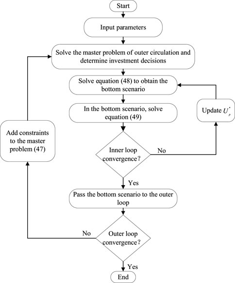
FIGURE 3. NCCG algorithm flowchart.

5 Case study

5.1 Parameter settings

In this article, it is first tested in a modified IEEE 33-node distribution system (Zhou et al., 2019) and then further applied in a 152-node 10 kV distribution system in a region. The example grid structure is shown in Figure 4 and Figure 5. The planning period is set to three stages, each lasting for 3a. The initial capacity of TS in the modified IEEE 33-node distribution system is 3.15 MVA, and the candidate main transformer capacities are 3.15MVA, 6.3 MVA, and 10 MVA; The initial capacity of TS in the 152-node distribution system is 10 MVA, and the candidate main transformer capacities are 6.3 MVA, 10 MVA, and 20 MVA; The cost of TS capacity increase is 500,000$/(MVA). The parameters of RIES candidate nodes and candidate equipment (Ehsan and Yang, 2019) can be found in Table 1 and Table 2. There are already biogas supply points built at the candidate nodes. The candidate lines and the parameters of the selected models are shown in Table 3 and Table 4, with a lifespan of 25a. Procurement of electricity from the power grid through the utilization of time-of-use tariffs can be observed in detail in Table 5 (Subramanian and Das, 2019) The constant price of biogas is set at 0.193 $/(kWh).

FIGURE 4

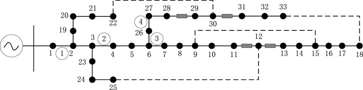
FIGURE 4. Modified IEEE 33-node system network structure.

FIGURE 5

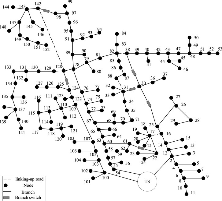
FIGURE 5. 152-node system network structure.

TABLE 1

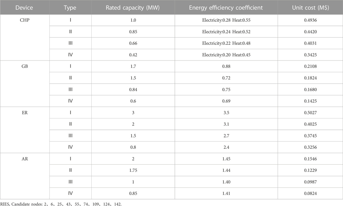
TABLE 1. Parameters of energy conversion equipment in RIES.

TABLE 2

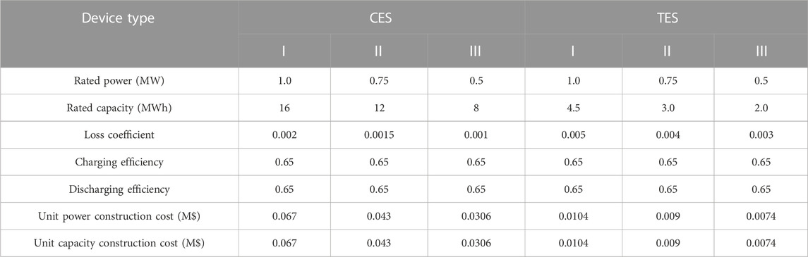
TABLE 2. Parameter of energy storage equipment in RIES.

TABLE 3

TABLE 3. Information of candidate lines.

TABLE 4

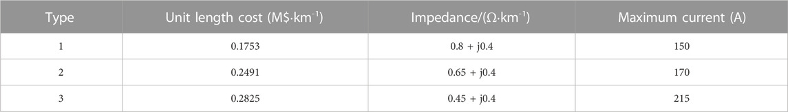
TABLE 4. Parameter of a line candidate model.

TABLE 5

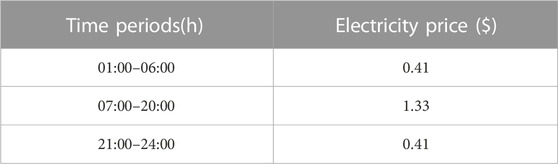
TABLE 5. Peak Valley electricity prices.

5.2 Scenario generation results

The setting of load parameters needs to take into account the impact of load development, seasonal factors, and other factors at each planning stage. Firstly, obtain the 8760h cold/hot/electrical load of a certain region through DesT software (DeST introduction, 2023). Then, a total of 1000 sets of data are generated through the implementation of Monte Carlo simulation. Subsequently, the enhanced k-means clustering methodology is employed to get the cooling, heating, and electricity loads for four representative days. The curves are depicted in Figure 6. Where Figure 6B and Figure 6D show significant changes in cold and heat loads, with high peaks and load-saving characteristics in summer and winter, respectively; The changes in cooling and heating loads in Figure 6A and Figure 6C are relatively gentle, with characteristics of spring and autumn loads. In terms of describing load uncertainty, this article considers that the maximum deviation of various load fluctuations is 10%, and the parameter $\mathrm{\Gamma }$ is set to 6.

FIGURE 6

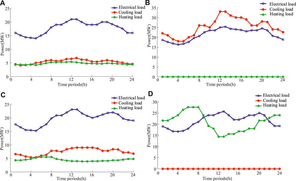
FIGURE 6. (A) Typical scenario 1; (B) Typical scenario 2; (C) Typical scenario 3; (D) Typical scenario 4.

5.3 Planning results

5.3.1 Modified IEEE 33-node example

This article sets up two comparative schemes based on whether to consider RIES or not. Among them, without considering RIES, the cooling and heating loads are converted into electrical loads using a thermoelectric energy efficiency coefficient of 2.5; When considering RIES, the optimized configuration combination of RIES devices is shown in Table 6. Based on four typical daily load scenarios, the proposed rural distribution network planning method with RIES was first tested in the modified IEEE 33-node system. The planning and operation outcomes of each stage are presented in Table 7. Where the numbers inside and outside the parentheses of the RIES column represent the configuration combination number and installation location of the RIES equipment; The numbers inside and outside the parentheses of the line represent the combination number and installation position of the line configuration; /represents no investment, the same applies later.

TABLE 6

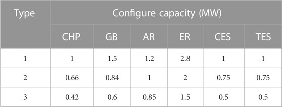
TABLE 6. Planning results of RIES equipment combination configuration.

TABLE 7

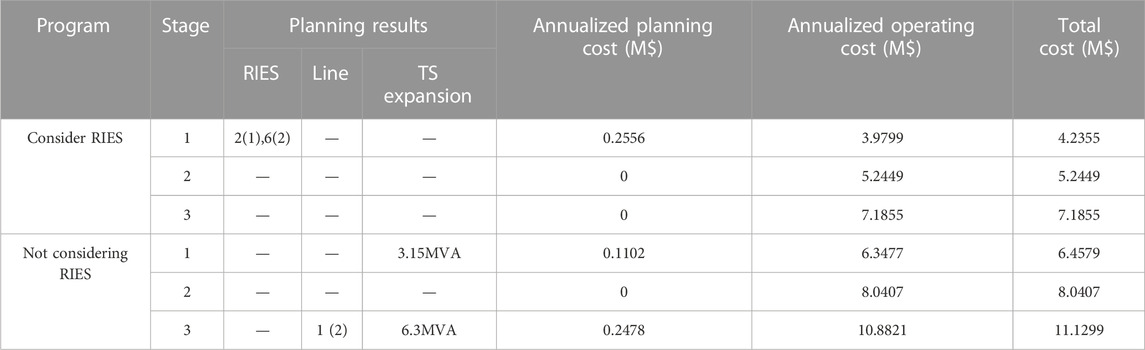
TABLE 7. Comparison of planning results for modified IEEE 33-node system.

When considering RIES, there is no need to expand or renovate the line and TS, and only two RIES were invested in planning phase 1; Without considering RIES, TS was increased by 3.15MVA in planning stage 1, and both the line and TS were upgraded and renovated in planning stage 3. After considering RIES, the total annualized planning cost has slightly decreased by approximately 13.2%. In terms of operational efficiency, considering RIES, the annual operating costs of each planning stage have decreased by approximately 35.35% compared to not considering RIES.

5.3.2 152-Node system calculation example

Based on four typical scenarios, further application is carried out in a 152-node system. The distribution network planning and operation results of each planning stage are depicted in Table 8.

TABLE 8

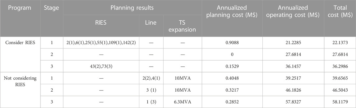
TABLE 8. Comparison of planning results for the 152-node system.

As can be seen from the planning results in Table 8, when considering RIES, it is only planned in stages 1 and 3, and the investment is mainly in stage 1, accounting for 85.59%; Without considering RIES, there are investments in line and TS expansion at all stages. The total annualized planning cost when considering RIES is approximately 1.05 times that when not considering RIES. The annualized cost during the initial planning stage (stage 1) is approximately 2.245 times that without considering RIES. In the sub-sequent planning stages (planning stages 2 and 3), under the same load growth rate, the annualized planning cost is about 25.2% of that without considering RIES, and the in-vestment period is delayed by one stage. It can be seen that when considering RIES, there is only a significant investment in the initial stage, and the subsequent investment reduction effect is significant. There are two main reasons for this. 1) Before the construction of RIES, the cooling and heating loads in rural areas were mainly supplied by electricity, and the absence of energy storage devices was observed in the system. Therefore, after considering the construction of RIES, the initial investment is large, but it also effectively transfers some of the power supply pressure of the distribution net-work; Without considering RIES, the initial stage is based on the planning of the existing power grid, so the investment is relatively low; 2) After the distribution network planning, due to the regulatory role of RIES, the energy supply curve has been effectively smoothed. And the supply pressure of various loads was allocated to corresponding equipment, alleviating the pressure of electricity load growth.

As can be noticed from the operational results in Table 8, the distribution network operation economy after considering RIES has shown good results. The total annualized operating cost decreased by approximately 41.16% compared to when RIES was not considered. RIES can store energy during electricity price valleys and release energy during peak hours while using biogas to replace a portion of electricity during peak hours can further reduce operating costs; When not taking into account the RIES, the operating cost of the system is solely dependent on the load and electricity price, resulting in reduced economic efficiency.

Furthermore, with regard to the regulation of the disparity between peak and valley levels in the power grid, a comparison is made between the electricity load curves before and after the planning. The results are shown in Figure 7 and Figure 8. The peak-to-valley ratio of Scenarios 1 and 3 has increased from 66.67% to 65.80% before planning to 83.07% and 83.51% after planning; The peak to valley ratio of scenarios 2 and 4 has increased from 64.98% to 64.85% before planning to 84.14% and 80.87% after planning. The peak-to-valley ratio of four typical scenarios has been improved to varying degrees.

FIGURE 7

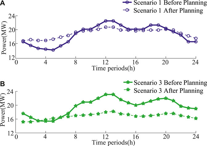
FIGURE 7. (A) Scenario 1 load comparison results in a 152-node system; (B) Scenario 3 load comparison results in a 152-node system.

FIGURE 8

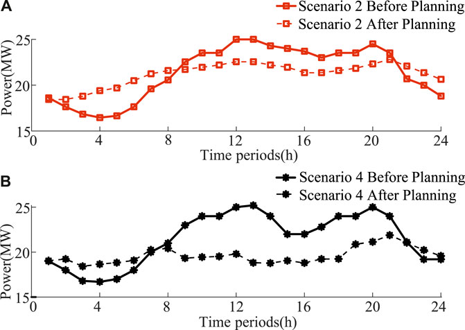
FIGURE 8. (A) Scenario 2 load comparison results in a 152-node system; (B) Scenario 4 load comparison results in a 152-node system.

Take Scenario 1 as an example to conduct a detailed analysis of the operating mechanism of RIES. Figure 9 and Figure 10 depict the cooling and heating output of RIES subsequent to the implementation of the planning phase. From Figure 9, it can be seen that 01:00 to 05:00 are the low periods of cooling load, during which AR is not activated and ER output is relatively high; Starting from 06:00, CES stops cold storage and ER output decreases to cooperate with AR cooling; CES starts cooling from 07:00, and after reaching a peak at 19:00, the cooling load begins to decrease. At 22:00, CES stops cooling and starts cooling storage again, resulting in a decrease in AR output and an increase in ER output.

FIGURE 9

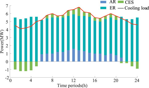
FIGURE 9. The cooling output of RIES after planning.

FIGURE 10

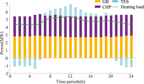
FIGURE 10. Heating output of RIES after planning.

As can be noticed from Figure 10, the heat load curve is relatively flat, and due to the fixed price of biogas. Therefore, there is almost no significant fluctuation in the output of GB and CHP. TES stores heat from 01:00 to 06:00 and 21:00 to 24:00 and begin to release heat from 07:00 to 20:00 to cooperate with GB, CHP for heating load, and AR heating.

5.4 Comparison with traditional solutions

Table 9 presents a comparison of the results between the robust planning scheme considering RIES and the traditional planning scheme in the IEEE 33-node scenario. From Table 9, it can be seen that: 1) The robust model incurs higher investment and operational costs in comparison to the deterministic model. This is because the robust model takes into account the uncertainty of the cooling/heating/electricity loads in the planning process and the planning decisions made are more conservative than the deterministic model. Similarly, there is an increase in operational expenses. The increase in operating cost is mainly in the area of energy purchase; 2) The robust model reduces the cost of regulation of the distribution network compared to the deterministic model. This is because there are more RIES inputs, and the operational cost of the grid can be effectively reduced by energy storage and peak shifting, and energy substitution. Therefore, the robust planning model presented in this article can not only play a good effect on peak and valley difference regulation but also has a certain resistance to fluctuation risk.

TABLE 9

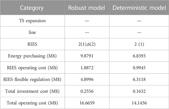
TABLE 9. Comparison of results between robust planning schemes considering RIES and traditional planning schemes.

5.5 Impact of uncertain parameters

To evaluate the flexibility of the proposed approach in relation to the cautiousness of planning schemes, five different sets of uncertain adjustment parameters were chosen for comparative simulation. The specific configurations of these parameters and the corresponding outcomes of the simulations are displayed in Table 10.

TABLE 10

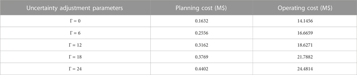
TABLE 10. Comparison of planning scheme results under different uncertainty adjustment parameters.

The data presented in Table 10 demonstrates that when the uncertainty adjustment parameter is set to 0, the robust planning model is equal to the Deterministic system. As the uncertainty parameters increase, the corresponding planning and operating costs increase. That is to say, when formulating the planning plan, more uncertainty is taken into account, resulting in a more conservative plan. With the increase of RIES in the planning scheme, the corresponding operating costs are also increasing.

6 Conclusion

In this article, a multistage robust planning approach is introduced for rural distribution networks that incorporate integrated energy stations. The method takes the distribution network as the main body, and the integrated energy station plays the role of regulation to alleviate the pressure of power supply in rural areas; the improved k-means clustering algorithm is employed to obtain multiple typical scenarios to improve the clustering efficiency. The method’s feasibility and effectiveness were evaluated using a modified version of the IEEE 33-node system, and then further based on a 152-node distribution system in a local area for practical application, the following conclusions are obtained.

1) The distribution network planning method proposed in this article, which takes into account RIES, has the advantage of reducing investment cycle and planning costs, although it has a relatively large investment in the initial planning stage. And as the planning period increases, its investment economy will also become more apparent. In terms of load regulation, RIES can effectively improve the peak-to-valley ratio of loads through the strategy of energy storage equipment storing energy during valley hours and releasing energy during peak hours.

2) The proposed model incorporates the consideration of load uncertainty. By continuously changing uncertainty parameters, the conservatism of the entire planning scheme can be flexibly adjusted. It is beneficial for planners to make a reasonable choice between operating costs and operational risks.

Data availability statement

The original contributions presented in the study are included in the article/Supplementary material, further inquiries can be directed to the corresponding author.

Author contributions

ZY: Conceptualization, Investigation, Resources, Software, Writing–original draft. HM: Conceptualization, Formal Analysis, Investigation, Resources, Visualization, Writing–original draft. FY: Methodology, Resources, Validation, Writing–review and editing. YLi: Software, Validation, Writing–original draft. YS: Data curation, Project administration, Writing–review and editing. BZ: Funding acquisition, Investigation, Writing–review and editing. ZZ: Investigation, Supervision, Writing–original draft. WH: Software, Writing–original draft. YLe: Software, Validation, Writing–original draft.

Funding

The author(s) declare that no financial support was received for the research, authorship, and/or publication of this article.

Conflict of interest

Authors ZY, HM, FY, YLi, YS, WH, and YLe were employed by Electric Power Research Institute of State Grid Hubei Co., Ltd. Authors BZ and ZZ were employed by State Grid Hubei Electric Power Co., Ltd.

Publisher’s note

All claims expressed in this article are solely those of the authors and do not necessarily represent those of their affiliated organizations, or those of the publisher, the editors and the reviewers. Any product that may be evaluated in this article, or claim that may be made by its manufacturer, is not guaranteed or endorsed by the publisher.

References

DeST introduction (2023). DeST introduction. Available at: http://dest.tsinghua.edu.cn/(Accessed July 4, 2023).

Google Scholar

Dong, F., Hou, Y., Li, W., and Wang, Y. (2022). Intelligent decision-making of distribution network planning scheme with distributed wind power generations. Int. J. Electr. Power and Energy Syst. 136, 107673. doi:10.1016/j.ijepes.2021.107673

CrossRef Full Text | Google Scholar

Ehsan, A., and Yang, Q. (2019). Scenario-based investment planning of isolated multi-energy microgrids considering electricity, heating and cooling demand. Appl. energy 235, 1277–1288. doi:10.1016/j.apenergy.2018.11.058

CrossRef Full Text | Google Scholar

Feng, Y., Zhang, W., Yin, S., Tang, H., Xiang, Y., and Zhang, Y. (2023). A collaborative stealthy DDoS detection method based on reinforcement learning at the edge of internet of things. IEEE Internet Things J. 10, 17934–17948. doi:10.1109/JIOT.2023.3279615

CrossRef Full Text | Google Scholar

Gan, W., Yan, M., Yao, W., Guo, J., Ai, X., Fang, J., et al. (2021). Decentralized computation method for robust operation of multi-area joint regional-district integrated energy systems with uncertain wind power. Appl. Energy 298, 117280. doi:10.1016/j.apenergy.2021.117280

CrossRef Full Text | Google Scholar

Ge, S., Liu, X., and Ge, L. (2018). Planning method of regional integrated energy system considering demand side uncertainty. Int. J. Emerg. Electr. Power Syst. 20 (1), 20180195. doi:10.1515/ijeeps-2018-0195

CrossRef Full Text | Google Scholar

Han, J., Zhang, L., and Li, Y. (2022). Spatiotemporal analysis of rural energy transition and upgrading in developing countries: the case of China. Appl. Energy 307, 118225. doi:10.1016/j.apenergy.2021.118225

CrossRef Full Text | Google Scholar

Heidari, S., and Fotuhi-Firuzabad, M. (2019). Integrated planning for distribution automation and network capacity expansion. IEEE Trans. Smart Grid 10 (4), 4279–4288. doi:10.1109/tsg.2018.2855218

CrossRef Full Text | Google Scholar

Huo, D., Gu, C., Greenwood, D., Wang, Z., Zhao, P., and Li, J. (2021). Chance-constrained optimization for integrated local energy systems operation considering correlated wind generation. Int. J. Electr. Power and Energy Syst. 132, 107153. doi:10.1016/j.ijepes.2021.107153

CrossRef Full Text | Google Scholar

International Energy Agency (2015). Air conditioning use emerges as one of the key drivers of global electricity-demand growth. Available at: https://www.iea.org/news/air-conditioning-use-emerges-as-one-of-the-key-drivers-ofglobal-electricity-demand-growth (Accessed July 4, 2023).

Google Scholar

Jiang, M., Liu, T., Goh, H., Zhang, D., Dai, W., Liu, J., et al. (2020). Estimation of operation cost of residential multiple energy system considering uncertainty of loads and renewable energies. IEEE Access 9, 4874–4885. doi:10.1109/access.2020.3046621

CrossRef Full Text | Google Scholar

Kim, M., and Ramakrishna, R. S. (2005). New indices for cluster validity assessment. Pattern Recognit. Lett. 26 (15), 2353–2363. doi:10.1016/j.patrec.2005.04.007

CrossRef Full Text | Google Scholar

Kou, X., and Li, F. (2018). Interval optimization for available transfer capability evaluation considering wind power uncertainty. IEEE Trans. Sustain. Energy 11 (1), 250–259. doi:10.1109/tste.2018.2890125

CrossRef Full Text | Google Scholar

Koutsoukis, N., and Georgilakis, P. (2019). A chance-constrained multistage planning method for active distribution networks. Energies 12 (21), 4154. doi:10.3390/en12214154

CrossRef Full Text | Google Scholar

Lei, Y., Wang, D., Jia, H., Chen, J., Li, J., Song, Y., et al. (2020). Multi-objective stochastic expansion planning based on multi-dimensional correlation scenario generation method for regional integrated energy system integrated renewable energy. Appl. energy 276, 115395. doi:10.1016/j.apenergy.2020.115395

CrossRef Full Text | Google Scholar

Li, H., Ren, Z., Fan, M., Li, W., Xu, Y., Jiang, Y., et al. (2022b). A review of scenario analysis methods in planning and operation of modern power systems: methodologies, applications, and challenges. Electr. Power Syst. Res. 205, 107722. doi:10.1016/j.epsr.2021.107722

CrossRef Full Text | Google Scholar

Li, H., Ren, Z., Trivedi, A., Srinivasan, D., and Liu, P. (2023). Optimal planning of dual-zero microgrid on an island towards net-zero carbon emission. IEEE Trans. Smart Grid, 1. doi:10.1109/TSG.2023.3299639

CrossRef Full Text | Google Scholar

Li, H., Ren, Z., Trivedi, A., Verma, P., Srinivasan, D., and Li, W. (2022a). A noncooperative game-based approach for microgrid planning considering existing interconnected and clustered microgrids on an island. IEEE Trans. Sustain. Energy 13 (4), 2064–2078. doi:10.1109/tste.2022.3180842

CrossRef Full Text | Google Scholar

Li, R., Wang, W., and Xia, M. (2017). Cooperative planning of active distribution system with renewable energy sources and energy storage systems. IEEE Access 6, 5916–5926. doi:10.1109/access.2017.2785263

CrossRef Full Text | Google Scholar

Moazeni, S., Miragha, A. H., and Defourny, B. (2018). A risk-averse stochastic dynamic programming approach to energy hub optimal dispatch. IEEE Trans. Power Syst. 34 (3), 2169–2178. doi:10.1109/tpwrs.2018.2882549

CrossRef Full Text | Google Scholar

Subramanian, V., and Das, T. K. (2019). A two-layer model for dynamic pricing of electricity and optimal charging of electric vehicles under price spikes. Energy 167, 1266–1277. doi:10.1016/j.energy.2018.10.171

CrossRef Full Text | Google Scholar

Wu, C., Gu, W., Jiang, P., Li, Z., Cai, H., and Li, B. (2017). Combined economic dispatch considering the time-delay of district heating network and multi-regional indoor temperature control. IEEE Trans. Sustain. Energy 9 (1), 118–127. doi:10.1109/tste.2017.2718031

CrossRef Full Text | Google Scholar

Wu, J., Yan, J., Jia, H., Hatziargyriou, N., Djilali, N., and Sun, H. (2016). Integrated energy systems. Appl. Energy 167, 155–157. doi:10.1016/j.apenergy.2016.02.075

CrossRef Full Text | Google Scholar

Yan, B., Yan, J., Li, Y., Qin, Y., and Yang, L. (2021). Spatial distribution of biogas potential, utilization ratio and development potential of biogas from agricultural waste in China. J. Clean. Prod. 292, 126077. doi:10.1016/j.jclepro.2021.126077

CrossRef Full Text | Google Scholar

Yan, M., Ai, X., Shahidehpour, M., Li, Z., Wen, J., Bahramira, S., et al. (2019). Enhancing the transmission grid resilience in ice storms by optimal coordination of power system schedule with pre-positioning and routing of mobile DC de-icing devices. IEEE Trans. Power Syst. 34 (4), 2663–2674. doi:10.1109/tpwrs.2019.2899496

CrossRef Full Text | Google Scholar

Zeng, B., and Zhao, L. (2013). Solving two-stage robust optimization problems using a column-and-constraint generation method. Operations Res. Lett. 41 (5), 457–461. doi:10.1016/j.orl.2013.05.003

CrossRef Full Text | Google Scholar

Zhou, Q., Shahidehpour, M., Yan, M., Wu, X., Alabdulwahab, A., and Abusorrah, A. (2019). Distributed secondary control for islanded microgrids with mobile emergency resources. IEEE Trans. Power Syst. 35 (2), 1389–1399. doi:10.1109/tpwrs.2019.2942269

CrossRef Full Text | Google Scholar