An adaptive time stepping stiffness confinement method for solving reactor dynamics equations

The stiffness confinement method (SCM) is frequently employed to solve the reactor dynamics equations because it confines the stiffness of the problem by frequency transformation. However, the balance between the error and efficiency of the SCM has not been well studied. This paper reports the error analysis of the SCM. The error by SCM is derived mathematically and written as integral error, driven by the integral of the frequency interpolation function. An easy-to-implement adaptive time-stepping (ATS) algorithm is proposed based on the error analysis by controlling the neutron flux amplitude error. First, a fine-step PKE is leveraged to estimate the second-order derivative of the flux amplitude-frequency, which is used to predict the error of the neutron flux amplitude. The low cost of solving the PKE incurs a negligible effect on the algorithm’s efficiency. Second, based on the error analysis, an error estimator proposed to determine an optimal time-step size for the neutron temporal-spatial equation. With a pre-set error tolerance, the ATS algorithm is exempted from the empirical selection of the time-step size in transient simulations. Numerical tests with TWIGL and modified 2D LMW benchmark problems show that the optimal time-step size effectively confines the local truncation error of the flux amplitude within the pre-set tolerance. The ATS algorithm yields a higher accuracy at a commensurate computational cost than calculations with fixed time-steps.

1 Introduction

Reactor dynamics equations (NDEs), such as the neutron temporal-spatial equation (NTSE) and the point kinetics equation (PKE), are employed to predict the transient behaviors of the neutron flux and precursors in a nuclear reactor. In the NDEs, the generation time of prompt and delayed neutrons involves multiple time scales. As these different time scales bring stiffness in the NDE, the time-step size must be sufficiently small to yield accurate results. The fine time-step causes a significant computational burden to the reactor dynamics calculations. Therefore, the stiffness confinement method (SCM) was proposed. In doing so, the SCM introduces the flux frequency and the precursor frequency to decouple the precursor equation from the NDE, thus confining the stiffness to the prompt neutron equation (Chao and Attard, 1985). Next, an exponential solution assumption decomposes the flux amplitude-frequency into the amplitude and shape frequencies (Park and Joo, 2015). By these means, the problem is transformed into a dynamic eigenvalue problem (EVP) that exhibits a similar equation form as that for the steady-state eigenvalue problem. Therefore, the dynamic EVP can be solved efficiently by power iteration and the non-linear iteration algorithm.

The SCM has already been applied in the PKE and the diffusion and transport NTSEs (Park and Joo, 2015; Tang et al., 2019). It has been demonstrated that the SCM can provide accurate and stable solutions. However, although the SCM enables solving the NTSE with a large time-step size, the computational cost of the NTSE at each time step is still high, especially for transport calculations. The adaptive time-stepping (ATS) algorithm has received much attention for further reducing computational costs. It allows transient solvers to optimally determine the time-step sizes according to the current transient state and the pre-set error tolerance. The algorithm improves the computational efficiency by allocating more time steps in time intervals where necessary. In addition, the ATS algorithm saves the trouble of empirically selecting the time-step size in transient simulations. Hence, ATS algorithms have been applied in solution methods to NTSE, such as the implicit Euler method, the quasi-static method, and the PKE-based SCM (Caron et al., 2017). However, an effective ATS algorithm for the three-dimensional SCM has yet to be developed because of the lack of comprehensive error analysis.

ATS algorithms are generally based on estimating and controlling of the local truncation error. Classically, the local truncation error $\epsilon$ of a numerical method of order $q$ can be expressed as (Tang et al., 2019):

$\epsilon \left(t\right)=\mathit{\Theta }\left(t\right)h^{q+1}+\mathit{O}\left(h^{q+2}\right)(1)$

where $t$ denotes the time, $\mathrm{\Theta }$ is the norm of the principal error function, and $h$ is the time-step size. Generally, $\mathrm{\Theta }$ is estimated with an error bound. The error bound is appropriated via the high-order derivative or even the Jacobian matrix of the solution. For lower complexity, $\mathrm{\Theta }$ can be assumed as constant between successive time steps and calculated by numerical differentiation. The numerical differentiation is computed using solutions from previous time steps (Caron et al., 2017). This approach does not require extra computation, but the predicted error may deviate significantly from the actual error. The deviation leads to a non-optimal time-step size and affects the efficiency of the ATS algorithm. Another practical ATS algorithm estimates the error by comparing the solution with a reference solution. With gradually reduced time-step size, the solution is rejected until the error between the computed solution and the reference solution reaches the pre-set tolerance. The adaptive time-step size is found by successively comparing solutions with two different time-step sizes and choosing the finer step solution as the reference one (Boffie and Pounders, 2018). Another approach is the embedded pair, which selects the time-step size by embedding low-order methods in the high-order method. For instance, a generalized Runge-Kutta method of fourth-order accuracy embeds a third-order solution to estimate the adaptive time-step size (Zimin and Ninokata, 1998). Although these ATS algorithms are easy to implement, the rejection-acceptance procedure calls for extra computation. Therefore, it is beneficial to develop an ATS algorithm that can efficiently and accurately control the time-step size for the SCM.

In this work, a theoretical error analysis of the SCM is performed. The theoretical analysis produces a mathematical error expression of the SCM. Further, an ATS algorithm is proposed by controlling the error of the neutron flux amplitude. In doing so, a fine-step PKE solver is used to evaluate high order derivatives of the neutron flux amplitude in the error expression. In addition, an error estimator based on the error expression is proposed and examined using benchmark problems. It is demonstrated that the ATS algorithm yields a higher accuracy at a commensurate computational cost than calculations with fixed time-steps.

The remainder of the paper proceeds as follows. Section 2 briefly describes the frequency-transformed NTSE and PKE. Solution methods to these equations are introduced in Section 3. In Section 4, the SCM's theoretical error analysis is performed, and an ATS algorithm based on the error analysis is proposed. Section 5 elaborates the coupling between the NTSE solver with the PKE solver. Section 6 illustrates the performance of error estimators and offers comparisons of the efficiency and accuracy between ATS and fixed time-stepping (FTS). Section 7 concludes the paper and points to directions for future research.

2 Frequency-transformation of dynamics models

The derivation of the SCM starts with the definition of the dynamic frequency. The dynamic frequency $\alpha \left(r,t\right)$ of a physical quantity $f\left(r,t\right)$ is defined as (Chao and Attard, 1985):

$\alpha \left(r,t\right)=\frac{1}{f\left(r,t\right)}\frac{\partial f\left(r,t\right)}{\partial t}r\in {\mathbb{R}}^3,t\in \mathbb{R}(2)$

where $r$ is the spatial variable and $t$ is the time variable. By introducing the dynamic frequency, a composite exponential function is employed to describe $f\left(r,t\right)$. Thus, the following exponential form of the solution is obtained:

$f\left(r,t\right)=f\left(r,t_0\right)e^{{\displaystyle \underset{t_0}{\overset{t}{\mathit{\int }}}}d{t}^{\prime }\alpha \left(r,t^{\prime }\right)}(3)$

Transient equations imposed with the dynamic frequency are called frequency-transformed equations. The frequency-transformed equations are solved by discretizing the time variable and searching $\alpha \left(r,t\right)$ iteratively.

For simplicity, we investigate the application of the SCM to the NTSE with diffusion approximation. Extending the methodology to neutron transport problems is not arduous (Park and Joo, 2015). Transient multi-group neutron diffusion equations with delayed neutron precursors are given as:

$\frac{1}{v_g}\frac{d{\phi }_g\left(r,t\right)}{dt}+\left[-\nabla \cdot D_g\left(r,t\right)\nabla +{\mathrm{\Sigma }}_{t,g}\left(r,t\right)\right]{\phi }_g\left(r,t\right)=\left[{\chi }_g\left(r\right)\left(1-\beta \right)Q\left(r,t\right)+{\displaystyle {\sum }_{g^{\prime }=1}^G}{\mathrm{\Sigma }}_{g^{\prime }-g}\left(r,t\right){\phi }_{g^{\prime }}\left(r,t\right)\right]+{\displaystyle {\sum }_{i=1}^I}{\chi }_{ig}{\lambda }_i{C}_i\left(r,t\right)g=1,\cdots ,G(4)$

$\frac{d{C}_i\left(r,t\right)}{dt}={\beta }_{i}Q\left(r,t\right)-{\lambda }_i{C}_i\left(r,t\right)i=1,\cdots ,I(5)$

where ${\phi }_g\left(r,t\right)$ represents the neutron flux of group $g$, $C_i\left(r,t\right)$ is the delayed neutron precursor concentration of precursor family $i$, and other notations are conventional. The fission source $Q$ is defined as:

$Q\left(r,t\right)={\displaystyle {\sum }_{g^{\prime }=1}^G}\nu {\mathrm{\Sigma }}_{f,g^{\prime }}\left(r,t\right){\phi }_{g^{\prime }}\left(r,t\right)(6)$

The neutron flux frequency is introduced to derive the frequency-transformed dynamics model:

${\omega }_g\left(r,t\right)\equiv \frac{1}{{\phi }_g\left(r,t\right)}\frac{\partial }{\partial t}{\phi }_g\left(r,t\right)(7)$

where ${\omega }_g\left(r,t\right)$ represents the neutron flux frequency which can be further split as ${\omega }_g\left(r,t\right)={\omega }_{S,g}\left(r,t\right)+{\omega }_T\left(t\right)$. The flux amplitude-frequency ${\omega }_T\left(t\right)$ represents a global quantity and is dependent only on time; the flux shape-frequency ${\omega }_{S,g}\left(r,t\right)$ is dependent on space, time, and energy. For normalization, a physics-based constraint on the shape-frequency is introduced as (Chao and Attard, 1985):

${\displaystyle \sum _{g=1}^G}{\displaystyle {\int }_V}dr\kappa {\mathrm{\Sigma }}_{f,g}\left(r,t\right){\phi }_g\left(r,t_0\right)e^{{\displaystyle \underset{t_0}{\overset{t}{\int }}}d{t}^{\prime }{\omega }_{S,g}\left(r,t^{\prime }\right)}=P\left(t_0\right)(8)$

where, $\kappa$ is the heat release per fission reaction, and $P\left(t_0\right)$ is the initial total power of the nuclear reactor. The constraint guarantees that the shape-frequency affects only the flux shape, not the total power. The power distribution $q\left(r,t\right)$ is defined as:

$q\left(r,t\right)={\displaystyle \sum _{g=1}^G}\kappa {\mathrm{\Sigma }}_{f,g}\left(r,t\right){\phi }_g\left(r,t_0\right)(9)$

The precursor concentration frequency is defined as:

${\mu }_i\left(r,t\right)\equiv \frac{1}{C_i\left(r,t\right)}\frac{\partial }{\partial t}{C}_i\left(r,t\right)(10)$

Introducing the frequency-transformation, the transient multi-group neutron diffusion equations and associated delayed neutron precursor equations are rewritten as:

$\left[-\nabla \cdot D_g\left(r,t\right)\nabla +{\mathrm{\Sigma }}_{t,g}\left(r,t\right)\right]{\phi }_g\left(r,t\right)+\frac{{\omega }_{S,g}\left(r,t\right)+{\omega }_T\left(t\right)}{v_g}{\phi }_g\left(r,t\right)=\left[{\chi }_g\left(r\right)\left(1-\beta \right)+{\displaystyle {\sum }_{i=1}^I}\frac{{\chi }_{ig}{\beta }_i{\lambda }_i}{{\mu }_i\left(r,t\right)+{\lambda }_i}\right]Q\left(r,t\right)+{\displaystyle {\sum }_{g^{\prime }=1}^G}{\mathrm{\Sigma }}_{g^{\prime }-g}\left(r,t\right){\phi }_{g^{\prime }}\left(r,t\right)g=1,...,G(11)$

${\mu }_i\left(r,t\right)C_i\left(r,t\right)={\beta }_{i}Q\left(r,t\right)-{\lambda }_i{C}_i\left(r,t\right)i=1,...,I(12)$

Equation 11 is the frequency-transformed temporal-spatial equation. Taking all frequencies in Eq. 11 to be zeros yields the static neutron diffusion equation:

$\left[-\nabla \cdot D_g\left(r,t_0\right)\nabla +{\mathrm{\Sigma }}_{t,g}\left(r,t_0\right)\right]{\phi }_g\left(r,t_0\right)=\frac{{\chi }_g\left(r\right)}{k_{\text{eff}}}{\displaystyle {\sum }_{g^{\prime }=1}^G}\nu {\mathrm{\Sigma }}_{f,g^{\prime }}\left(r,t_0\right){\phi }_{g^{\prime }}\left(r,t_0\right)+{\displaystyle {\sum }_{g^{\prime }=1}^G}{\mathrm{\Sigma }}_{g^{\prime }-g}\left(r,t_0\right){\phi }_{g^{\prime }}\left(r,t_0\right)g=1,\cdots ,G(13)$

The adjoint equations corresponding to Eq. 13 are:

$\left[-\nabla \cdot D_g\left(r,t_0\right)\nabla +{\mathrm{\Sigma }}_{t,g}\left(r,t_0\right)\right]{\phi }_g^{†}\left(r,t_0\right)=\frac{\nu {\mathrm{\Sigma }}_{f,g}\left(r,t_0\right)}{k_{\text{eff}}}{\displaystyle {\sum }_{g^{\prime }=1}^G}{\chi }_{g^{\prime }}\left(r\right){\phi }_{g^{\prime }}^{†}\left(r,t_0\right)+{\displaystyle {\sum }_{g^{\prime }=1}^G}{\sum }_{g-g^{\prime }}\left(r,t_0\right){\phi }_{g^{\prime }}^{†}\left(r,t_0\right)g=1,\cdots ,G(14)$

The left-hand side of Eq. 14 is the adjoint diffusion-absorption operator, which is self-adjoint, and the right-hand side is the adjoint fission-scattering operator. Eqs 13, 14 are both EVPs, which can be solved by power iteration.

The PKE is a lumped-parameter model used to analyze the dynamic behaviors of the flux amplitude while neglecting the flux shape. As will be shown, this model is beneficial in the error analysis of the SCM. The PKE results by integrating Eqs 4, 5 weighted with the initial adjoint flux. The resulting equations are:

$\frac{\mathrm{d}n\left(t\right)}{\mathrm{d}t}=\frac{\rho \left(t\right)-\beta }{\mathrm{\Lambda }}n\left(t\right)+{\displaystyle \sum _{i=1}^I}{\lambda }_i{C}_i\left(t\right)(15)$

$\frac{\mathrm{d}{C}_i\left(t\right)}{\mathrm{d}t}=\frac{{\beta }_i}{\mathrm{\Lambda }}n\left(t\right)-{\lambda }_i{C}_i\left(t\right)i=\mathrm{1,2},...,I(16)$

in which the notations are conventional thus are neglected for brevity. Readers can find detailed definitions of the dynamic parameters in Appendix-A. Correspondingly, the neutron density frequency for the PKE is be given by:

$\omega \left(t\right)\equiv \frac{1}{n\left(t\right)}\frac{\mathrm{d}n\left(t\right)}{\mathrm{d}t}(17)$

which can also be called the amplitude-frequency. The frequency-transformed point kinetics model is expressed as:

$\omega \left(t\right)=\frac{\rho \left(t\right)-\beta }{\mathrm{\Lambda }}+\frac{1}{n\left(t\right)}{\displaystyle \sum _{i=1}^I}{\lambda }_i{C}_i\left(t\right)(18)$

The precursor concentration equations are identical to Eq. 16.

3 Solution method for frequency-transformed equations

Introducing the dynamic eigenvalue $k_{\mathrm{D}}$ in Eq. 11, the equation can be transformed into an EVP:

$\left[-\nabla \cdot D_g\left(r,t\right)\nabla +{\mathrm{\Sigma }}_{t,g}^{\prime }\left(r,t\right)\right]{\phi }_g\left(r,t\right)=\frac{{\chi }_g^{\prime }\left(r\right)}{k_D}Q\left(r,t\right)+{\displaystyle {\sum }_{g^{\prime }=1}^G}{\mathrm{\Sigma }}_{g^{\prime }-g}\left(r,t\right){\phi }_{g^{\prime }}\left(r,t\right)g=1,...,G(19)$

where, ${\mathrm{\Sigma }}_{t,g}^{\prime }\left(r,t\right)$ is the dynamic total cross-section, and ${\chi }_g^{\prime }\left(r\right)$ is the dynamic fission spectrum, which are respectively defined as:

${\sum }_{t,g}^{\prime }\left(r,t\right)\equiv {\mathrm{\Sigma }}_{t,g}\left(r,t\right)+\frac{{\omega }_{S,g}\left(r,t\right)+{\omega }_T\left(t\right)}{v_g}(20)$

${\chi }_g^{\prime }\left(r\right)\equiv {\chi }_g\left(r\right)\left(1-\beta \right)+{\displaystyle {\sum }_{i=1}^I}\frac{{\chi }_{ig}{\beta }_i{\lambda }_i}{{\mu }_i\left(r,t\right)+{\lambda }_i}(21)$

The dynamic frequencies rendering the maximum eigenvalue $k_{\mathrm{D}}$ equal to 1are the solutions to Eq. 19. It is noted that the dynamic eigenvalue $k_{\mathrm{D}}$ can be expressed as a non-linear function of the flux amplitude-frequency ${\omega }_T$. Thus, the dynamic frequencies are solved iteratively using power iteration and the non-linear iteration algorithms. The non-linear iteration algorithm employed in this paper is the $k-\omega$ iteration, as shown in Algorithm 1:

Algorithm 1. SCM for time-spatial equations.

function SpatialSolverSCM(t_N, h, XS)

 {tn}←{0 : h : t_N } Time steps

 ${\stackrel{\sim }{\phi }}_g\left(r,t_0\right)$,k_eff ← EVPSolver(XS(t₀))

 ${\stackrel{\sim }{\phi }}_g\left(r,t_0\right)\leftarrow \frac{P_0}{{\int }_{V}dr\stackrel{\sim }{q}\left(r,t_0\right)}{\stackrel{\sim }{\phi }}_g\left(r,t_0\right)$ Normalize initial flux

 $C_i\left(r,t_0\right)\leftarrow \frac{{\beta }_i}{{\lambda }_i}Q\left(r,t_0\right)$

 ${\omega }_T\left(t_0\right),{\omega }_{S,g}\left(r,t_0\right),{\mu }_i\left(r,t_0\right)\leftarrow 0$

 while n ≤ N do

    ${\omega }_T^{\left(0\right)}\left(t_n\right)\leftarrow {\omega }_T\left(t_{n-1}\right)$

    ${\omega }_{S,g}^{\left(0\right)}\left(r,t_n\right)\leftarrow {\omega }_{S,g}\left(r,t_{n-1}\right)$

    $C_i^{\left(0\right)}\left(r,t_n\right)\leftarrow C_i\left(r,t_{n-1}\right)$

   KOmegaIteration(··· )

   $P_n\leftarrow {\int }_{V}drq\left(r,t_n\right)$

 end while

 return $\left\{{\phi }_g\left(r,t_n\right)\right\},\left\{C_i\left(r,t_n\right)\right\},\left\{\omega \left(r,t_n\right)\right\}$

end function

function EVPSolver(XS)

 % Any existing neutron transport or diffusion EVP solver

 return ${\stackrel{\sim }{\phi }}_g\left(r\right)$,k_eff

end function

function KOmegaIteration( )

 % Input and output variables are omitted

 while m≤M do

  ${\stackrel{\sim }{\phi }}_g^{\left(m\right)}\left(r,t_n\right),k_D^{\left(m+1\right)}$←EVPSolver(XS′(t₀))

  ${\omega }_T^{\left(m+1\right)}\left(t_n\right)\leftarrow \text{Update\hspace{0.17em}}{\omega }_T^{\left(m+1\right)}\left(t_n\right)$ based on Eq. 22

  ${\stackrel{\sim }{\phi }}_g^{\left(m+1\right)}\left(r,t_n\right)\leftarrow \frac{P_{n-1}}{{\int }_{V}dr\overline{q}\left(r,t_n\right)}{\stackrel{\sim }{\phi }}_g^{\left(m\right)}\left(r,t_n\right)$

  ${\omega }_{S,g}\left(t_n\right)\leftarrow \frac{1}{h}\mathit{ln}\left(\frac{{\phi }_g^{\left(m+1\right)}\left(r,t_n\right)}{{\phi }_g\left(r,t_{n-1}\right)}\right)$

  ${\phi }_g\left(r,t_n\right)\leftarrow {\widehat{\phi }}_g^{\left(m+1\right)}\left(r,t_n\right)e^{\frac{{\omega }_T^{\left(m+1\right)}\left(t_n\right)+{\omega }_T\left(t_{n-1}\right)}{2}}h$

  $C_i^{\left(m+1\right)}\left(r,t_n\right)\leftarrow \text{Update\hspace{0.17em}}{C}_i^{\left(m\right)}\left(r,t_n\right)$ based on Eq. 26

  ${\mu }_i^{\left(m+1\right)}\left(r,t_n\right)\leftarrow \text{Update\hspace{0.17em}}{\mu }_i^{\left(m\right)}\left(r,t_n\right)$ based on Eq. 28

  if $\left|k_D^{\left(m+1\right)}-1\right|<\epsilon$ then

   break

  end if

  XS′(tn)← Update dynamics cross-sections based Eqs. 20 and 21

 end while

end function

where $XS$ denotes all coefficients in Eqs 11, 12, including cross-sections and dynamic parameters, $h$ is the time step size, and $t_N$ is the last time point. If not otherwise specified, $n$ and $m$ denote the time step index and iteration index, respectively. In this study, the finite difference method (FDM) is applied to solve the EVP of the neutron diffusion equation, and the solutions are ${\stackrel{\sim }{\phi }}_g\left(r,t\right)$ and the associated eigenvalue $k_{\mathrm{D}}$. Besides, other spatial discretization algorithms are also applicable, such as the nodal method (Abo et al., 2008) and the finite element method.

The amplitude-frequency is updated using the secant method (Chao and Attard, 1985):

${\omega }_T^{\left(m+1\right)}\left(t_n\right)={\omega }_T^{\left(m\right)}\left(t_n\right)+\left[{\omega }_T^{\left(m-1\right)}\left(t_n\right)-{\omega }_T^{\left(m\right)}\left(t_n\right)\right]\frac{1-k_{\mathrm{D}}^{\left(m\right)}}{k_{\mathrm{D}}^{\left(m-1\right)}-k_{\mathrm{D}}^{\left(m\right)}}(22)$

The iteration continues until the dynamic eigenvalue converges to 1. According to Eq. 8, normalization is necessary to update the shape-frequency with the normalized neutron flux ${\widehat{\phi }}_g\left(r,t_n\right)$:

${\widehat{\phi }}_g\left(r,t_n\right)=\frac{P\left(t_{n-1}\right)}{\sum _{g=1}^G{\int }_{V}dr\kappa {\mathrm{\Sigma }}_{f,g}\left(r,t_n\right){\stackrel{\sim }{\phi }}_g\left(r,t_n\right)}{\stackrel{\sim }{\phi }}_g\left(r,t_n\right)(23)$

Such a normalization enforces the total power contributed by the normalized flux to equal the power of the previous time step, which ensures that the shape-frequency is independent of the flux amplitude. Thus, the update formula of the shape-frequency is:

${\overline{\omega }}_{S,g}\left(r,t_n\right)=\frac{1}{\Delta t_n}\ln \left[\frac{{\widehat{\phi }}_g\left(r,t_n\right)}{{\phi }_g\left(r,t_{n-1}\right)}\right](24)$

where $\Delta t_n=t_n-t_{n-1}$, and ${\overline{\omega }}_{S,g}\left(r,t_n\right)$ is the average shape-frequency in $\left[t_{n-1},t_n\right]$. According to Eq. 3, the update formula for the actual neutron flux is:

${\phi }_g\left(r,t_n\right)={\phi }_g\left(r,t_{n-1}\right)e^{\frac{{\omega }_T\left(t_n\right)+{\omega }_T\left(t_{n-1}\right)}{2}\Delta t_n+{\overline{\omega }}_{S,g}\left(r,t_n\right)\Delta t_n}={\widehat{\phi }}_g\left(r,t_n\right)e^{\frac{{\omega }_T\left(t_n\right)+{\omega }_T\left(t_{n-1}\right)}{2}\Delta t_n}(25)$

When the actual neutron flux is solved, the precursor concentration is calculated by:

$C_i\left(r,t_n\right)=C_i\left(r,t_{n-1}\right)e^{-{\lambda }_i\Delta t_n}+{\beta }_i{e}^{-{\lambda }_i\Delta t_n}{\displaystyle {\int }_{t_{n-1}}^{t_n}}\Delta Q\left(r,t\right)e^{{\lambda }_{i}t}dt(26)$

Suppose that the fission source changes linearly within $\left[t_{n-1},t_n\right]$, the expression of the fission source is given by:

$Q\left(r,t\right)=Q\left(r,t_{n-1}\right)+\frac{Q\left(r,t_n\right)-Q\left(r,t_{n-1}\right)}{\Delta t_n}\left(t-t_{n-1}\right)(27)$

According to Eq. 12, the precursor frequency is calculated by:

${\mu }_i\left(r,t\right)=\left\{\begin{array}{ll}{\beta }_i\frac{Q\left(r,t\right)}{C_i\left(r,t\right)}-{\lambda }_i& C_i\left(r,t\right)\ne 0\\ 0& C_i\left(r,t\right)=0\end{array}\right.(28)$

The resulting flux and precursor frequencies are then used to update the dynamic cross-section. For the case of the PKE, the non-linear frequency-transformed equations can be solved using Algorithm 2:

Algorithm 2. SCM for PKE.

function PKESolverSCM(t_N, h, IC, DP)

 $\left\{t_n\right\}\leftarrow \left\{0:h:t_N\right\}$ Time steps

 $n\left(t_0\right),C_i\left(t_0\right),\omega \left(t_0\right)\leftarrow IC$ Initial conditions

 while n ≤ N do

  ${\omega }^{\left(0\right)}\left(t_n\right)\leftarrow \omega \left(t_n-1\right)$

   $C_i^{\left(0\right)}\left(t_n\right)\leftarrow C_i\left(t_{n-1}\right)$

  while m≤M do

   $n^{\left(m+1\right)}\left(t_n\right)\leftarrow n\left(t_n\right)e^{\frac{{\omega }^{\left(m\right)}\left(t_n\right)+\omega \left(t_{n-1}\right)}{2}h}$

   ω^(m+1)(tn)←Update ω^(m)(tn) based on Eq. 31

   C(m+1)(tn)←Update $C_i^{\left(m\right)}\left(t_n\right)$ based on Eq. 33

   if $\left|f\right|<\epsilon$ then

    break

   end if

  end while

 end while

 return {n(tn)}, {Ci(tn)}, {ω(tn)}

end function

where $IC$ represents the initial conditions, and $DP$ is the dynamic parameters in Eqs 16, 18. With a linear approximation of the neutron density frequency, the neutron density can be updated by:

$n\left(t_n\right)=n\left(t_{n-1}\right)e^{\frac{\omega \left(t_n\right)+\omega \left(t_{n-1}\right)}{2}h}(29)$

in which $\omega$ is solved iteratively. According to Eq. 18, function $f$ is introduced:

$f\left(t_n\right)=-\omega \left(t_n\right)+\frac{\rho \left(t_n\right)-\beta }{\mathrm{\Lambda }}+\frac{1}{n\left(t_{n-1}\right)e^{\frac{\omega \left(t_n\right)+\omega \left(t_{n-1}\right)}{2}h}}{\displaystyle \sum _{i=1}^I}{\lambda }_i{C}_i\left(t_n\right)(30)$

In this case, $\omega$ is solved with the secant method until $f\left(t_n\right)=0$:

${\omega }^{\left(m\right)}\left(t_n\right)={\omega }^{\left(m-1\right)}\left(t_n\right)-\frac{\left[{\omega }^{\left(m-1\right)}\left(t_n\right)-{\omega }^{\left(m-2\right)}\left(t_n\right)\right]}{\left[f^{\left(m-1\right)}\left(t_n\right)-f^{\left(m-2\right)}\left(t_n\right)\right]}{f}^{\left(m-1\right)}\left(t_n\right)(31)$

The precursor concentration $C_i\left(t_n\right)$ can be determined using the analytical solution to Eq. 16:

$C_i\left(t_n\right)=C_i\left(t_{n-1}\right)e^{-{\lambda }_i\Delta t_n}+\frac{{\beta }_i}{\mathrm{\Lambda }}{e}^{-{\lambda }_i\Delta t_n}{\displaystyle {\int }_{t_{n-1}}^{t_n}}n\left(t\right)e^{{\lambda }_{i}t}dt(32)$

Assuming that the neutron density changes linearly with time, Eq. 32 is transformed into:

$C_i\left(t_{n+1}\right)=C_i\left(t_n\right)e^{-{\lambda }_i\Delta t_n}+\frac{\beta }{\mathrm{\Lambda }{\lambda }_i^2\Delta t_n}\left\{\begin{array}{l}\left[-\Delta t_n{\lambda }_{i}n\left(t_n\right)-n\left(t_n\right)+n\left(t_{n+1}\right)\right]e^{-{\lambda }_i\Delta t_n}\\ +\Delta t_n{\lambda }_{i}n\left(t_{n+1}\right)+n\left(t_n\right)-n\left(t_{n+1}\right)\end{array}\right\}(33)$

4 Error analysis and error estimator

In the SCM, polynomial functions are used to interpolate the exact frequency. The interpolation points are frequencies obtained by solving frequency-transformed equations at different time points. Figure 1 offers a schematic view of errors in the numerical integral. As shown in the figure, when a polynomial interpolation function ${\omega }^{\prime }$ replaces the original function ${\omega }^{*}$, error is introduced when integrating over the time interval. The error can be estimated by the difference in the covered area between the original function and the interpolation function in Figure 1.

FIGURE 1

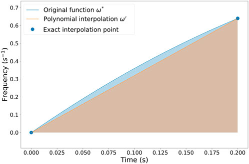
FIGURE 1. Illustration of integral error and zero-point bias with linear approximation.

With the foregoing considerations, we define the integral error contributing to truncation error in the SCM:

Definition 1. (Integral error): The integral error ${\epsilon }_{\mathit{int}}$ is defined as the difference between the integral using the original function ${\omega }^{*}$ and the integral using the polynomial interpolation ${\omega }^{\prime }$ of ${\omega }^{*}$:

${\epsilon }_{\mathit{int}}\equiv {\displaystyle {\int }_{\Delta t}}{\omega }^{*}\left(t\right)dt-{\displaystyle {\int }_{\Delta t}}{\omega }^{\prime }\left(t\right)dt(34)$

The interpolation error at $t$ is ${\omega }^{*}\left(t\right)-{\omega }^{\prime }\left(t\right)$, which is the difference between the original function providing the interpolation points and the interpolating polynomial. Assume that ${\omega }^{\prime }\left(t\right)$ is the (degree $n$ or less) interpolating polynomial fitting the $n+1$ points $\left\{\left(t_0,{\omega }^{*}\left(t_0\right)\right),\cdots ,\left(t_n,{\omega }^{*}\left(t_n\right)\right)\right\}$. Without loss of generality, it is assumed that the frequency is $\left(n+1\right)$-order differentiable due to the smooth variation of reactivity $\rho$ in Eq. 18. The interpolation error is then (Zhang et al., 2017):

${\omega }^{*}\left(t\right)-{\omega }^{\prime }\left(t\right)=\frac{1}{\left(n+1\right)!}{\omega }^{*\left(n+1\right)}\left({\xi }_t\right){\displaystyle {\prod }_{i=0}^n}\left(t-t_i\right)(35)$

where ${\xi }_t$ lies between $\left[t_0,t_n\right]$, and ${\omega }^{*\left(n+1\right)}$ is the $\left(n+1\right)$-order derivative of the frequency. When the neutron density frequency is interpolated with a linear function within a time step, by applying the mean value theorem of integrals, the integral error in $\left[t_{n-1},t_n\right]$ is obtained as:

${\epsilon }_{\mathit{int}}={\displaystyle {\int }_{t_{n-1}}^{t_n}}{\omega }^{*}\left(t\right)dt-{\displaystyle {\int }_{t_{n-1}}^{t_n}}{\omega }^{\prime }\left(t\right)dt=-\frac{1}{12}{\omega }^{*\left(2\right)}\left(\xi \right){\left(t_n-t_{n-1}\right)}^3\xi \in \left[t_{n-1},t_n\right](36)$

Because the exact value of $\xi$ is uncertain, Eq. 36 can be used to provide error bounds to the solutions. Hence, the optimal time step is given using the error estimator:

$h\text{′}=\sqrt[3]{\frac{12{\epsilon }_{tol}}{{\omega }^{\left(2\right)}\left(\xi \right)}}h\text{′}\in {\mathbb{R}}^{+}(37)$

5 Coupling of the NTSE solver with the PKE predictor

Based on the above discussions, one can select the optimal time steps for the SCM based on Algorithms 3, 4:

Algorithm 3. Adaptive time stepping SCM based on PKE predictor.

function SpatialSolverAdaptiveSCM(t_N, h_max, h_min, ε_tol, XS)

 t₀←0

 ϕ˜_g(r,t₀),k_eff ← EVPSolver(XS(t₀))

 ${\phi }_g\left(r,t_0\right)\leftarrow \frac{P_0}{{\int }_{V}dr\stackrel{\sim }{q}\left(r,t_0\right)}{\stackrel{\sim }{\phi }}_g\left(r,t_0\right)$ Normalize initial flux

 $C_i\left(r,t_0\right)\leftarrow \frac{{\beta }_i}{{\lambda }_i}Q\left(r,t_0\right)$

 ω_T (t0),ω_S,g (r,t0),µi(r,t0)←0

 for t_n ≤t_N do n++

  $t_n^{\prime }\leftarrow t_{n-1}+h_{\max }$

  ICn−1,DPn−1← Initialized IC and DP

  h_n←TimeStepSelection(ε_tol,h_max,h_min,IC_n−1,DP_n−1)

  tn←tn−1 +hn

  ${\omega }_T^{\left(0\right)}\left(t_n\right)\leftarrow {\omega }_T\left(t_{n-1}\right)$

  ${\omega }_{S,g}^{\left(0\right)}\left(r,t_n\right)\leftarrow {\omega }_{S,g}\left(r,t_{n-1}\right)$

  $C_i^{\left(0\right)}\left(r,t_n\right)\leftarrow C_i\left(r,t_{n-1}\right)$

  KOMegaIteration(···)

  $P_n\leftarrow {\int }_{V}drq\left(r,t_n\right)$

 end for

 return {ϕg {r,tn},{Ci(r,tn)}, {ω(r,tn)}

end function

Algorithm 4. Adaptive time step selection based on PKE.

function TimeStepSelection(ε_tol, h_max, h_min, IC, DP)

 $h_{sub}\leftarrow \frac{h_{\max }}{K}\text{Sub}-\text{step\hspace{0.17em}for\hspace{0.17em}PKE}$

 {ω_k}←PKESolverSCM(h_max,h_sub,IC, DP)

 $\left\{{\omega }_k^{\left[2\right]}\right\}\leftarrow \frac{{\omega }_{k-1}2{\omega }_k+{\omega }_{k+1}}{h_{sub}^2}$

 ${\omega }^{\left[2\right]}\leftarrow \mathit{max}\left\{\left|{\omega }_k^{\left[2\right]}\right|\right\}$

 h′←ErrorControl(ε_tol,ω^[2])

 h←max{hmin, min{h′, hmax}}

 return h

end function

function ErrorControl(ε_tol, ω^[2])

 $h\sqrt[3]{\frac{12{\epsilon }_{tol}}{{\omega }^{\left[2\right]}}}$

 return h′

end function

Algorithm 4 shows the time-step selection subroutine with the error estimator demonstrated in Eq. 37. An optimal time-step size is chosen using the error estimator to control the local error within the pre-set error tolerance in this subroutine. Algorithm 3 is obtained by embedding Algorithm 4 in Algorithm 1.

The key to the ATS algorithm is to solve the PKE in the time interval $\left[t_{n-1},t_{n-1}+h_{\max }\right]$ before solving the NTSE. In solving the PKE, dynamic parameters and initial conditions are generated using the solution of the NTSE and the initial adjoint flux. To make appropriate predictions, the following assumptions are used for solving the PKE:

• The flux shape is fixed in the prior interval and the solution ${\phi }_g\left(r,t_{n-1}\right)$ is used to evaluate all necessary parameters and initial conditions;

• All dynamic parameters are constant in the prior interval except the reactivity $\rho \left(t\right)$;

• $\rho \left(t\right)$ is a linear function in the prior interval, while $\rho \left(t_{n-1}\right)$ and $\rho \left(t_{n-1}+h_{\max }\right)$ are evaluated based on Supplementary Eq. 4.

The SCM is also applied to solve the PKE because it directly provides the frequency for error estimation.

6 Numerical Results

In this section, the efficiency and accuracy of the ATS algorithm are tested by comparing it with FTS calculation. We examine the time stepping algorithm in the TWIGL problem and the modified LMW-2D problem. The TWIGL problem represents a transient case with step perturbation, and the LMW problem involves smooth reactivity insertions with more complicated geometrical layout that that of the TWIGL problem. The combination of the two problems can be utilized to examine the performance of the ATS algorithm under different transient scenarios.

The cross-sections and dynamic parameters of the two problems are presented in Appendix-B. The reference solutions are obtained by fine time-step size calculations. We apply the ATS algorithm to the problems with specified error tolerance. For comparisons, we also adopt FTS calculations with the same number of time steps as those used to produce the ATS results to evaluate the accuracy improvements of using the ATS algorithm. For ease of description, in these discussions we denote ATS with a tolerance of x% as ATS-x%, and denote FTS with the time step of y ms as FTS-y ms.

6.1 TWIGL

The TWIGL benchmark problem is one quarter of a 2D reactor core consisting of three kinds of fuel materials, as shown in Figure 2 (Kennedy and Riley, 2012).

FIGURE 2

FIGURE 2. Layout of TWIGL benchmark problem.

The TWIGL benchmark problem includes two different reactivity insertion cases: a simple ramp case and a composite case. The composite case is adopted to validate the ATS algorithm, which is shown in Table 1. The transient durations for both cases are 0.5 s. Note that perturbations occur only in Material 1; the other materials remain in their initial conditions. The initial power distribution is shown in Figure 3.

TABLE 1

TABLE 1. Transient cases in TWIGL benchmark problem.

FIGURE 3

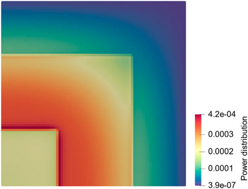
FIGURE 3. Initial power distribution for TWIGL.

In the TWIGL problem, the pre-set maximum and minimum time-step sizes are chosen as 50 and 1 ms, respectively. Figure 4A compares ATS-0.5% and FTS-20 ms. Figure 4B presents the adaptive time-step size. As shown in Figure 4A, the power curve of ATS agrees well with the reference solution, especially shortly after the step points. Step perturbations are introduced at 0.2 and 0.4 s. Accordingly, the ATS algorithm automatically refines step sizes shortly after step points but otherwise uses a coarse step size. Such a time step adjustment intelligently allocates time steps and spends more computational resources on the interval with rapid changes.

FIGURE 4

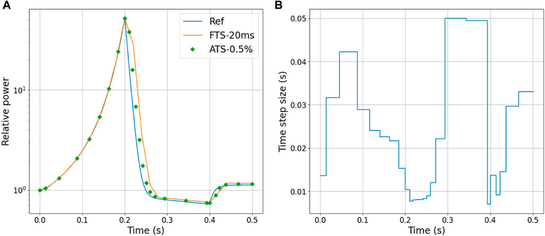
FIGURE 4. Comparison of ATS-0.5% and FTS-20 ms in TWIGL (A) Core power (B) Time-variant adaptive time-step size.

Figure 5A, B compare the results of ATS-0.1% and FTS-12.5 ms. The performance is similar to that in the previous error tolerance setting.

FIGURE 5

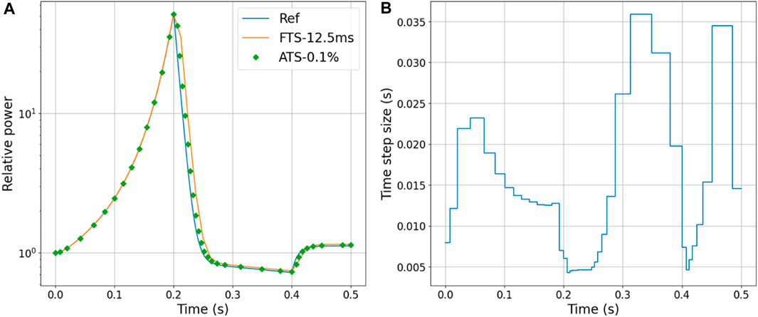
FIGURE 5. Comparison of ATS-0.1% and FTS-12.5 ms in TWIGL (A) Core power (B) Time-variant adaptive time-step size.

Table 2 summarizes the global core power error at different time step points. The ATS algorithm significantly improves the computational accuracy when the same number of time steps is used, with an error reduction of up to 40∼50%. The comparison of ATS-0.5% and FTS-12.5 ms in Table 2 indicates that the ATS algorithm can reduce by 37% the computational time of the FTS calculation with similar numerical accuracy. More significant gains can be expected for large-scale neutron transport problems.

TABLE 2

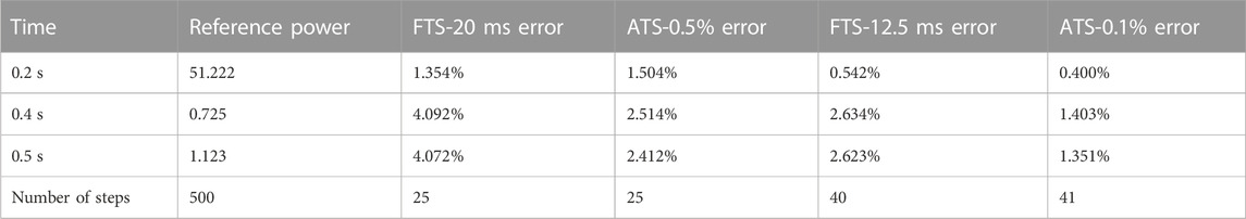
TABLE 2. Comparison of global amplitude error between ATS and FTS in TWIGL.

6.2 Modified 2D-LMW

The second 2D benchmark problem is modified from the 3D LMW (Langenbuch, Maurer, Werner) problem without thermal-hydraulic feedback to match the simulation code used in the paper (Kennedy and Riley, 2012). The reactor core is a simplified pressurized water reactor containing two kinds of fuel assemblies and two groups of control rods (CR), as shown in Figure 6.

FIGURE 6

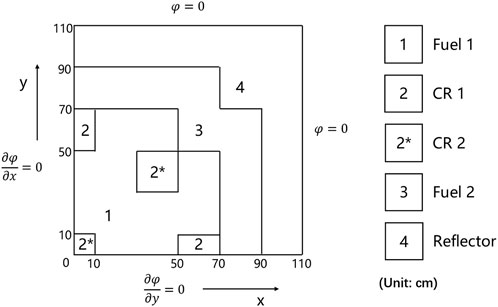
FIGURE 6. Layout of modified LMW-2D benchmark problem.

The modified 2D LMW problem is designed to model a reactivity insertion case, as shown in Table 3. This case is the superposition of ramp perturbations in different regions, by perturbing materials in CR 1 and CR 2. The initial power distribution is illustrated in Figure 7.

TABLE 3

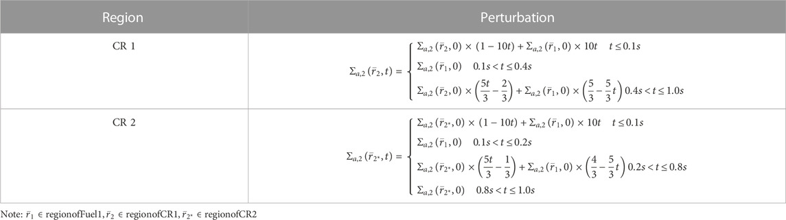
TABLE 3. Perturbations in modified LMW-2D benchmark problem.

FIGURE 7

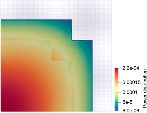
FIGURE 7. Initial power distribution for modified 2D-LMW (Only non-zero power displayed).

For the modified 2D-LMW, Figures 8, 9 present a comparison between the results of the ATS and FTS calculations. In Figure 8A, the error of the power peak, which appears at 0.4 s, is 905.02 and 3344.92 for ATS and FTS, respectively. In Figure 9A, the error of the power peak is 316.87 and 2219.20. The noticeable improvement in the accuracy of the power peak demonstrates the efficacy of the ATS algorithm.

FIGURE 8

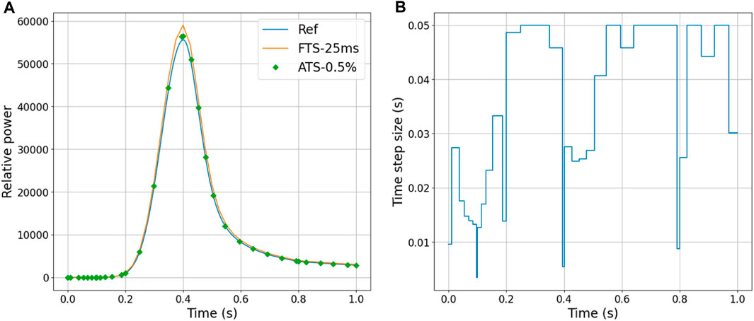
FIGURE 8. Comparison of ATS-0.5% and FTS-25 ms in modified 2D-LMW (A) Core power (B) Time-variant adaptive time-step size.

FIGURE 9

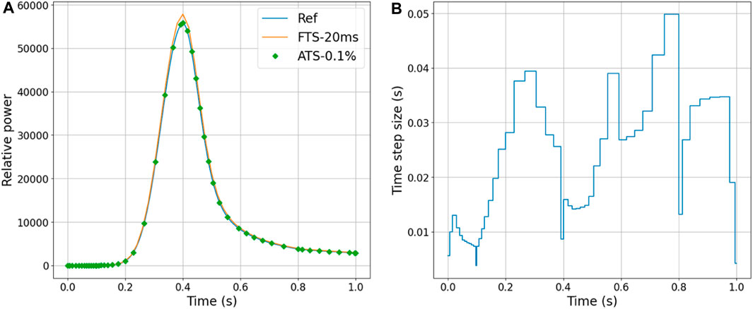
FIGURE 9. Comparison of the ATS-0.1% and FTS-20 ms in modified 2D-LMW (A) Core power (B) Time-variant adaptive time-step size.

Figure 10 presents the relative spatial error at 0.4s for ATS and FTS. We can observe that the error distribution is fairly uniform in both cases, but the accuracy of ATS is higher than that of FTS.

FIGURE 10

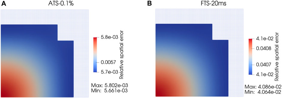
FIGURE 10. Comparison of relative spatial error at 0.4 s between ATS-0.1% and FTS-20 ms. (A) ATS-0.1%; (B) FTS-20 ms.

Table 4 summarizes the global core power error. The results show that the numerical accuracy can be improved significantly. For example, comparing FTS-20 ms and ATS-0.1%, the error reduction can be up to 90%∼95%. The core power increases by more than four orders of magnitudes from the initial power, whose variation is much wider than that in the TWIGL problem, but there is no step perturbation. Thus, continuity of frequency enables superior error control.

TABLE 4

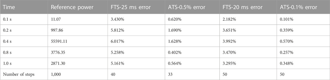
TABLE 4. Comparison of global amplitude error between ATS and FTS in modified 2D-LMW.

7 Conclusion

In this work, we perform theoretical and numerical error analyses of the SCM. By expressing the error term using integral error, the mathematical expression of the amplitude error is derived. The integral error is caused by using a polynomial function to represent the exact solution. Based on theoretical analysis, we develop an efficient and easy-to-implement ATS algorithm based on the PKE predictor. A fine-step PKE solver is used to rapidly evaluate high order derivatives of the neutron flux amplitude in the theoretical error expression. The high-order derivatives are used to determine the optimal time-step size for the NTSE. A time step error-estimator for this ATS algorithm is derived, and numerical validation indicates that the ATS is satisfactory in performance and easy to implement.

The accuracy and computational cost of ATS and FTS are examined using benchmark problems. Comparisons show that the ATS algorithm can achieve higher accuracy with the same number of time steps, and significantly improve computational efficiency in the NTSE. It was found that the ATS algorithm significantly improves the computational accuracy when the same number of time steps is used, with error reductions of up to 40%∼50% for the TWIGL benchmark and up to 90%∼95% for the LMW benchmark. With similar numerical accuracy, the ATS algorithm can reduce by 37% the computational time of the FTS calculation. Future work is to apply the adaptive SCM to 3D neutron transport problems.

Data availability statement

The raw data supporting the conclusion of this article will be made available by the authors, without undue reservation.

Author contributions

DW: Conceptualization, Formal analysis, Methodology, Validation, Writing–original draft. WX: Formal analysis, Methodology, Resources, Writing–review and editing. ZD: Supervision, Writing–review and editing. TZ: Conceptualization, Funding acquisition, Methodology, Writing–review and editing.

Funding

The authors declare that no financial support was received for the research, authorship, and/or publication of this article.

Conflict of interest

The authors declare that the research was conducted in the absence of any commercial or financial relationships that could be construed as a potential conflict of interest.

Publisher’s note

All claims expressed in this article are solely those of the authors and do not necessarily represent those of their affiliated organizations, or those of the publisher, the editors and the reviewers. Any product that may be evaluated in this article, or claim that may be made by its manufacturer, is not guaranteed or endorsed by the publisher.

Supplementary material

The Supplementary Material for this article can be found online at: https://www.frontiersin.org/articles/10.3389/fenrg.2023.1284230/full#supplementary-material

References

Aboanber, A. E., and Hamada, Y. M. (2008). Generalized Runge–Kutta method for two-and three-dimensional space–time diffusion equations with a variable time step. Ann. Nucl. Energy 35 (6), 1024–1040. doi:10.1016/j.anucene.2007.10.008

CrossRef Full Text | Google Scholar

Ban, Y., Endo, T., and Yamamoto, A. (2012). A unified approach for numerical calculation of space-dependent kinetic equation. J. Nucl. Sci. Technol. 49 (5), 496–515. doi:10.1080/00223131.2012.677126

CrossRef Full Text | Google Scholar

Boffie, J., and Pounders, J. M. (2018). An adaptive time step control scheme for the transient diffusion equation. Ann. Nucl. Energy 116, 280–289. doi:10.1016/j.anucene.2018.02.044

CrossRef Full Text | Google Scholar

Caron, D., Dulla, S., and Ravetto, P. (2017). Adaptive time step selection in the quasi-static methods of nuclear reactor dynamics. Ann. Nucl. Energy 105, 266–281. doi:10.1016/j.anucene.2017.03.009

CrossRef Full Text | Google Scholar

Chao, Y. A., and Attard, A. (1985). A resolution of the stiffness problem of reactor kinetics. Nucl. Sci. Eng. 90 (1), 40–46. doi:10.13182/nse85-a17429

CrossRef Full Text | Google Scholar

Kennedy, D., and Riley, D. (2012). Romes Desert Frontiers. Routledge.

Google Scholar

Park, B. W., and Joo, H. G. (2015). Improved stiffness confinement method within the coarse mesh finite difference framework for efficient spatial kinetics calculation. Ann. Nucl. Energy 76, 200–208. doi:10.1016/j.anucene.2014.09.029

CrossRef Full Text | Google Scholar

Tang, C., Bi, G., and Yang, B. (2019). Application of stiffness confinement method in transient neutron transportation calculation. Atomic Energy Sci. Technol. 53 (7), 1202. doi:10.7538/yzk.2018.youxian.0836

CrossRef Full Text | Google Scholar

Wanner, G., and Hairer, E. (1996). Solving ordinary differential equations II, 375. New York: Springer Berlin Heidelberg.

Google Scholar

Zhang, T., Wang, Y., Lewis, E. E., Smith, M. A., Yang, W. S., and Wu, H. (2017). A three-dimensional variational nodal method for pin-resolved neutron transport analysis of pressurized water reactors. Nucl. Sci. Eng. 188 (2), 160–174. doi:10.1080/00295639.2017.1350002

CrossRef Full Text | Google Scholar

Zimin, V. G., and Ninokata, H. (1998). Nodal neutron kinetics model based on nonlinear iteration procedure for LWR analysis. Ann. Nucl. Energy 25 (8), 507–528. doi:10.1016/s0306-4549(97)00078-9

CrossRef Full Text | Google Scholar