Scheduling of the HVAC system in a real commercial building considering equipment cycling and rebound effects

Commercial buildings consume a large portion of energy and the heating, ventilation, and air conditioning (HVAC) system is the major contributor to this high consumption. Though there are many reported works on the optimal scheduling of HVAC systems, practical considerations such as equipment cycling and possible rebound effects are rarely considered. This paper provides insights into the optimal scheduling of the HVAC system in an actual 3-floor commercial building where the cycling and rebound effects are addressed in the optimization. The experimental results prove that energy cost reduction can be achieved while ensuring temperature comfort and longer life expectancy of the HVAC. The results also show that considering the cycling and rebounds will affect the potential cost reduction.

1 Introduction

Buildings’ energy consumption has increased in recent years to represent a major part of the primary energy consumption. According to the latest statistics from U.S. Energy Information Administration (EIA), the combined residential and commercial buildings are estimated to consume around 40% of the total primary energy (EIA, 2023). The Heating, Ventilation, and Air Conditioning (HVAC) is the main reason that drives the consumption, accounting for about 44% of the building energy consumption (Tian, 2022). Therefore, modeling and optimizing HVAC systems have drawn attention.

The Building models can be generally classified into physics-based models (white box), data-driven models (black box), and hybrid models (gray box). In physics-based models, underlying first principles are used to model the building dynamics while in data-driven models, sensor data from the building automation systems are used. In hybrid models, simplified physics-based methods are used where the parameters of the models are identified using empirical data.

Physics-based models usually require the identification of physical parameters that range from the identification of equivalent lumped parameters in simplified models to complex parameter identification via the use of building geometry layouts, material types, equipment types, and operational schedules in detailed building models. In Jindal et al. (2018), simplified heat balance equations, characterizing the operation of fan coil units,were used to form the bases of a mixed integer linear programming (MILP) problem that minimizes the energy cost of a university building. Other researchers used detailed physics-based model predictive controller (MPC) for HVAC scheduling (Žáčeková et al., 2014; Sturzenegger et al., 2015). It was found that the challenge against the deployment of physics-based MPC is the time, cost, and effort to capture the dynamic features of the building. In addition, the demanding process of building model and calibration must be repeated for each building if more than one building will be controlled (Žáčeková et al., 2014). The significant modeling effort explains the reason why unoptimized rule-based methods are the most common scheduling mechanisms in commercial building automation systems.

Due to these reasons, some researchers tried to develop and use data-driven models for the control of commercial HVAC systems. In Smarra et al. (2018), regression trees and random forests were used as data-driven models for building energy optimization. The authors showed that data-driven predictive control can provide comparable performance with respect to control based on a perfectly known mathematical model. Linear regression and cubic functions were used in Hao et al. (2016) to approximate the temperature dynamics and fan power consumption of a variable air volume box. The models were used in setting the bidding strategies of a commercial building participating in the market.

In an attempt to combine the virtues of both methods and to compensate for the inaccuracy of data-driven models, some researchers explored the use of hybrid models (Ma et al., 2014; Kannan et al., 2019; Vishwanath et al., 2019). In Ma et al. (2014), the authors developed simplified nonlinear models for the thermal zones of the building. Then, state feedback linearization was used to develop a linear model that can be used by the model predictive controller (MPC). In Vishwanath et al. (2019), the authors deployed their prior knowledge of some physical parameters of the system as well as data coming from the building management system to formulate a MILP problem to optimize the cooling consumption of a large commercial building.

With the fast development of demand response programs for commercial buildings, the rebound effect has become a practical issue (Tian et al., 2021). Grid-interactive building refers to those that temporarily raise their HVAC temperature setpoints to reduce power consumption in response to grid signals. The rebound effect is the high power rebound that occurs after the setpoint is restored to the nominal value. The rebound effect of multiple buildings can be stacked when the coordination of cycling is lacking. These practical issues can have a great effect on the lifetime of the equipment and demand response performances, yet, proper cycling strategies are rarely studied. In addition, if not properly addressed, they can counter-affect the resulting cost reduction which is the main objective of the reported work. This happens because the rebound effect might introduce load peaks that in turn can increase the total consumption cost of the building operator, given the fact that many building managers are subjected to monthly peak time-of-use tariffs, known as demand charge costs (DukeEnergy, 2020).

Therefore, this paper presents a low-dimensional data-driven model and conventional optimal scheduling formulation of an actual 3-floor building to minimize the energy cost. The conventional formulation might result in cycling and system peak problems. So, the paper presents a potential solution to these problems while resulting in cost minimization as well. Real-world results of both cases are provided and discussed.

2 Building modeling

Building modeling is an important step for the optimization of the HVAC system. Usually, building models are used to mimic and generate the temperature and consumption dynamics of the building, that is, used as an oracle/model for the optimizer while evaluating different possible decision variables. The building under consideration is an actual 3-floor office/classroom building. According to the DOE classification, the building is considered a medium office building. The building has more than 100 offices that are distributed among different floors. The test building structure, including both the room sectioning and the thermal zone sectioning, is shown in Figure 1. It is equipped with advanced chilled-beam technology as the main air distribution system. Each group of rooms is supplied by pre-processed air coming from the variable air volume box (VAV) and the VAV boxes of each floor are supplied from an air handling unit (AHU). The scheduling of the AHUs controls the building’s temperature. Finally, the AHUs are fed from the central chiller of the university campus.

FIGURE 1

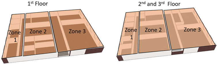
FIGURE 1. Floor plan and thermal zone sectioning of the test building.

As most commercial buildings are equipped with a building management system that stores historical data of different sensors of the building and HVAC system, data-based models arise as viable options that can be developed directly without the need to have in-depth knowledge about the different components of the building and HVAC system. Linear models are adopted in this work. The advantages of linear data-driven models include reduced complexity and compatibility with numerical optimization. Two data-driven models are developed to mimic the behavior of in-door building temperature and energy consumption. The control input to the system is the HVAC schedule O.

2.1 In-door temperature model

A linear regression model is used to develop the building temperature. The adopted features for the models are the HVAC schedule O, outside ambient temperature T_amb and the building temperature at the previous time step $T_{\mathit{BLD}}^{t-1}$. Though the selected features do not directly include the set-point temperature, it is implicitly included in the schedule O. In commercial buildings, the schedule O reflects a temperature set point that the chiller and the cooling coil should achieve. According to the (ASHRAE) standards, the On status can mean a working hour temperature set-point of 74°F or 75°F while the Off status means a setback temperature of 80°F. The temperature model is illustrated by (1) where β_i represents the temperature regression coefficients and β₀ is the intercept.

$T_{\mathit{BLD}}^t=T_{\mathit{BLD}}^{t-1}\cdot {\beta }_1+T_{\mathit{amb}}^t\cdot {\beta }_2+O^t\cdot {\beta }_3-{\beta }_0(1)$

2.2 HVAC consumption model

A similar model for the HVAC consumption is adopted and the consumption model is described by (2) where γ_i represents the power consumption regression coefficients and γ₀ is the intercept.

$P^t=T_{\mathit{BLD}}^{t-1}\cdot {\gamma }_1+T_{\mathit{amb}}^t\cdot {\gamma }_2+O^t\cdot {\gamma }_3-{\gamma }_0(2)$

3 Optimal HVAC scheduling

3.1 Basic formulation—Synchronized scheduling

First, a formulation is used where the objective is to minimize the electricity cost of the building by controlling the switching on/off status O of the AHUs. In this section, the monitored variable is the building temperature which represents the average temperature of all rooms in the building T_BLD. It is assumed that the AHUs work in a synchronous way (following the same schedule). These assumptions are common practices in many university campuses around the United States. Thus, the problem is formulated as an integer linear programming where the optimization problem is formulated as follows:

$\underset{O}{\min }{\displaystyle \sum _{t=1}^T}{c}^t\cdot P^t(\mathrm{3a})$

$s.t.T_{\mathit{lower}}\le T_{\mathit{BLD}}^t\le T_{\mathit{upper}}(\mathrm{3b})$

$O^{t+1}\ge O^t-O^{t-1}(\mathrm{3c})$

$1-O^{t+1}\ge O^{t-1}-O^t(\mathrm{3d})$

Where: Eq. 3a represents the objective of minimizing the energy cost where c is the time of use (ToU) tariff and P is the power consumed per unit of time by the HVAC system. Constraint (3b) states that the average building temperature should be always maintained between a lower comfort level and an upper comfort level. The comfort bounds are different during the day between working and non-working hours. Constraints (3c) and (3d) put limits on the minimum up and down times to reduce the wear and tear due to the switching on/off. These constraints are commonly used in the literature (Vrettos and Andersson, 2015; Tian et al., 2020). 30 min was set as the minimum up/down times. The temperature and power consumption at the next time step are obtained using the regression model as described by (1, 2).

3.2 Practical asynchronous formulation

The previous formulation may cause several practical issues which are: Rebound effect: the commonly used synchronized operation of the AHUs can cause power spikes. When all the AHUs are turned off simultaneously, the temperature in all rooms will increase simultaneously, and when the AHUs are turned on in the next time step, a large increase in the chilled water consumption will be induced to maintain the temperature within the bounds. This is similar to the typical rebound phenomenon observed in demand response programs when a larger peak is introduced in the system when the off-peak signal is sent. The presence of power spikes can have negative consequences on the mechanical equipment as well as the electrical equipment. In addition, the presence of power spikes can eliminate the savings generated during the turn-off periods and may increase the demand charge costs of the building. Temperature deviations: Since different parts of the buildings are subjected to different heat gains and may have different wall structures, using the same schedule might result in temperature deviations. For example, the upper floor receives a direct hit from the Sun during the middle of the day so this floor typically has much lower inertia compared to other floors and its temperature will rise quickly when the AHU is turned off, compared to other floors. Excessive cycling: though the basic formulation includes a limit on the minimum up and down times, excessive cycling of the AHUs can happen during moderate temperature days. This is because the optimizer will tend to turn on and off more often to minimize the cost. If the minimum up and down time is set to be a long period to avoid excessive cycling, it will reduce potential savings that can be obtained. This happens because the optimizer will avoid turning off the AHUs since a long minimum downtime means that the AHU will be off for an extended time which might result in temperature deviations. This is particularly true during hot days.

To consider these practical issues, first, the temperature dynamics of the AHUs are captured separately where each AHU will have its own temperature model according to (4). The average temperature of each AHU is a function of its previous temperature (the temperature of all rooms served by the AHU) and its own schedule as well as the outside temperature. As for the building consumption, there is no way to know the consumption of each of the AHUs separately as the chilled water meter shows only the total consumption. Therefore, the building power consumption model will be a function of the average temperature of the AHUs, outside temperature, as well as their individual schedules are given by (5) where α_i represents the power consumption regression coefficients in this case.

$T_{\mathit{AHU}}^t=T_{\mathit{AHU}}^{t-1}\cdot {\delta }_1+T_{\mathit{amb}}^t\cdot {\delta }_2+O_{\mathit{AHU}}^t\cdot {\delta }_3-{\delta }_0(4)$

$\begin{array}{ll}\hfill P^t& =average\left(T_{\mathit{AHU1}}^{t-1},T_{\mathit{AHU2}}^{t-1},T_{\mathit{AHU3}}^{t-1}\right)\cdot {\alpha }_1+T_{\mathit{amb}}^t\cdot {\alpha }_2\hfill \\ \hfill & +O_{\mathit{AHU1}}^t\cdot {\gamma }_3+O_{\mathit{AHU2}}^t\cdot {\gamma }_4+O_{\mathit{AHU3}}^t\cdot {\gamma }_5-{\gamma }_0\hfill \end{array}(5)$

$T_{\mathit{lower}}\le T_{\mathit{AHU}}^t\le T_{\mathit{upper}}(6)$

${\displaystyle \sum _{t=1}^{N_i}}|O_i^{t+1}-O_i^t|\le N_{\mathit{cycle}},i\in \left\{N_H\right\}(7)$

${\displaystyle \sum _{t=1}^{N_H}}{O}_i^t\ge N_{on},t\in \left\{N_t\right\}(8)$

In addition to separate temperature models of each of the AHUs, the previous constraints have been modified as follows: Constraint (6) considers the average temperature of the rooms served by different AHUs separately. It ensures that the average temperature of the different AHUs is within the bounds. Constraint (7) is used to limit the number of cycles of the AHU by ensuring that the total number of switching cycles during the operation day is less than a certain number of cycles N_cycle. This number is a factor to be decided by the building operator. To avoid the simultaneous switching off of the AHUs, constraint (8) is used to ensure that at each time step, there will be a certain minimum number of AHUs N_on that will be on out of the total number of AHUs N_H. This constraint helps smooth the load profile of the building and limits loading spikes.

4 Results

The optimization problem is resolved for real-world scenarios where the basic formulation will first be tested then the asynchronous practical formulation will be evaluated. For real-world scenarios, the regression model is trained using actual data from the building automation system. The weather forecast for the next day is obtained through an Application Program Interface (API) with NOAA weather forecast. To evaluate the effectiveness of the proposed formulation, the obtained costs will be compared to a standard non-test day of the building operation. Since the consumption will be affected by the outside temperature and it is hard to find two actual days with the exact ambient temperature, a similar day criterion (Sangrody et al., 2020) is adopted to ensure a fair comparison. A similar day is selected based on the minimum ambient temperature squared error between test days and other days in the same month. Finally, the building is subjected to Duke energy time of use tariff (ToU) (DukeEnergy, 2020) with the on-peak period between 12:00–21:00 p.m. Detailed building parameters and test settings are summarized in Table 1.

TABLE 1

TABLE 1. Regression model parameters.

4.1 Experimental results—Synchronous scheduling

In this test, the regression model is trained using 2 months of actual data and the obtained parameters are summarized in Table 2. The root means squared error (RMSE) for the temperature model is 0.1 and the RMSE error for the power model is 14.9. The data is coming from the building automation system with a 15-min resolution. The ambient temperature for the optimized test day is shown in Figure 2. The minimum up and down times was set to two time steps (30 min). Figure 3 depicts a comparison between the expected behavior using the regression model and the actual behavior of the building using the optimized schedule. Figure 3 also shows the average temperature of the rooms served by the different AHUs. The figure depicts the synchronous behavior of the scheduling where the temperature increases/decreases in all the AHUs simultaneously. The results show that the regression model is able to track the pattern but it underestimates the temperature and the energy consumption. The actual deviation in temperature is less than 0.5–1°F. Figure 3 also shows that the temperature deviation is different among the AHUs. This is because different heat gains affect different AHUs (i.e., the heat gain from the Sun increases as we go up).

TABLE 2

TABLE 2. Regression model parameters.

FIGURE 2

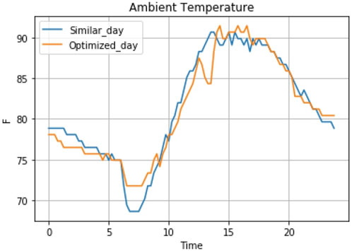
FIGURE 2. Ambient temperature profiles of the test day and a similar day.

FIGURE 3

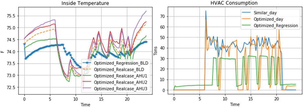
FIGURE 3. Optimized building temperature and power consumption under the synchronous scheduling method.

Figure 3 shows that there are multiple cycles (turning on and off) during the test day which represents a concern for the building operator as it will reduce the lifetime of the mechanical equipment. For other moderate temperature test days, excessive cycling was observed as the optimizer was trying to minimize the cost by more frequently turning on and off the equipment. These results were not shown due to space limitations. Figure 3 also shows that there is a spike in consumption whenever the building is turned off during the middle of the day since the building is trying to maintain the temperature after the building is heated up during the turn-off period. Also, these spikes partially contributed to the transient of the PI controller at the lower level of the control sequence of the equipment. Whenever a turn-on control signal is initiated after a turn-off period, the PI controller overshoots before settling down.

Finally, the energy and cost savings obtained using the optimized schedule are compared to a similar unoptimized day. The closest day to the test day and its consumption are shown in Figure 2 and Figure 3. It is obvious that the 2 days are very close to each other. The numerical results show that the optimized schedule will result in 115.9 kWh energy reduction (25.4%) and $11.96 cost reduction (31.2%), indicating the ability of a low dimensional model to achieve high savings without the need for extra complexities. Although the basic optimization formulation can result in excessive cycling and load peaks.

4.2 Experimental results—Asynchronous scheduling

In this case study, the practical formulation discussed in section III is used. In this case study, different schedules for the different AHUs are used. The maximum number of allowed cycles during working hours is 6 cycles and the minimum number of operating AHUs at any time instant is two AHUs. The performance of the building was also compared to a non-optimized day using the similar day criterion applied before. The left subplot of Figure 4 illustrates the average temperature behaviors of the rooms/offices served by the different AHUs. The figure shows that on average there is no temperature deviation above 74°F has occurred. The temperature behavior also shows the alternating behavior of the schedules where there is no simultaneous turning off of the AHUs (i.e., the temperatures do not go up simultaneously at the same time). This is because only one AHU of the three AHUs is allowed to turn off at a time. Also, the figure shows that the average temperature does not go up and down many times during the middle of the day. This is a direct result of the maximum number of cycles constraint. The alternating behavior of the turn-off procedure and limits on the number of cycles resulted in a smoother consumption profile as shown in the right subplot of Figure 4 where we can see the absence of large power spikes shown before. Also, these constraints ensure that there will always be a minimum load applied to the chiller (source of cooled water) as shown in the figure (i.e., the entire system never shuts down during working hours). This helps ensure a longer life expectancy for the equipment. Finally, when comparing the numerical results to similar day consumption, the proposed algorithm results in an energy reduction of 60.53 kWh (18.4%) and cost reduction of $4.59 (19.5%).

FIGURE 4

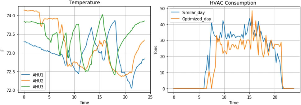
FIGURE 4. Optimized AHU temperature profiles and total HVAC power consumption under the asynchronous scheduling method.

5 Conclusion

This paper addresses the power rebound issue in grid-interactive buildings. An asynchronous cycling method is proposed to ensure a smooth consumption profile. The performances of the proposed low-dimensional regression model and optimization method were validated through an experiment on a 3-floor commercial building. The objective of the optimization problem was to minimize the cost of the chilled water consumption while the building is subjected to Duke Energy’s time-of-use tariff. The case study results showed that the proposed method can 1) achieve lower electricity cost under TOU; 2) effectively mitigate the rebound effect by optimizing the equipment cycling; and 3) increase the life expectancy of AHU equipment. The future work is to enhance the modeling accuracy by incorporating more features and non-linear characteristics among them.

Data availability statement

The original contributions presented in the study are included in the article/Supplementary Material, further inquiries can be directed to the corresponding author.

Author contributions

SF: Writing–original draft. QS: Writing–review and editing. GT: Writing–review and editing. AP: Writing–review and editing.

Funding

The author(s) declare that no financial support was received for the research, authorship, and/or publication of this article.

Acknowledgments

The authors sincerely acknowledge the contribution of all individuals, reviewers, and editors for their contribution towards the production of this manuscript.

Conflict of interest

The authors declare that the research was conducted in the absence of any commercial or financial relationships that could be construed as a potential conflict of interest.

Publisher’s note

All claims expressed in this article are solely those of the authors and do not necessarily represent those of their affiliated organizations, or those of the publisher, the editors and the reviewers. Any product that may be evaluated in this article, or claim that may be made by its manufacturer, is not guaranteed or endorsed by the publisher.

References

DukeEnergy (2020). Commercial/industrial rate schedules.

Google Scholar

EIA (2023). Monthly energy review september 2023.

Google Scholar

Hao, H., Corbin, C. D., Kalsi, K., and Pratt, R. G. (2016). Transactive control of commercial buildings for demand response. IEEE Trans. Power Syst. 32, 774–783. doi:10.1109/tpwrs.2016.2559485

CrossRef Full Text | Google Scholar

Jindal, A., Kumar, N., and Rodrigues, J. J. (2018). A heuristic-based smart hvac energy management scheme for university buildings. IEEE Trans. Industrial Inf. 14, 5074–5086. doi:10.1109/tii.2018.2802454

CrossRef Full Text | Google Scholar

Kannan, T., Lork, C., Tushar, W., Yuen, C., Wong, N. C., Tai, S., et al. (2019). Energy management strategy for zone cooling load demand reduction in commercial buildings: a data-driven approach. IEEE Trans. Industry Appl. 55, 7281–7299. doi:10.1109/tia.2019.2930599

CrossRef Full Text | Google Scholar

Ma, Y., Matuško, J., and Borrelli, F. (2014). Stochastic model predictive control for building hvac systems: complexity and conservatism. IEEE Trans. Control Syst. Technol. 23, 101–116. doi:10.1109/tcst.2014.2313736

CrossRef Full Text | Google Scholar

Sangrody, H., Zhou, N., and Zhang, Z. (2020). Similarity-based models for day-ahead solar pv generation forecasting. IEEE Access 8, 104469–104478. doi:10.1109/access.2020.2999903

CrossRef Full Text | Google Scholar

Smarra, F., Jain, A., De Rubeis, T., Ambrosini, D., D’Innocenzo, A., and Mangharam, R. (2018). Data-driven model predictive control using random forests for building energy optimization and climate control. Appl. energy 226, 1252–1272. doi:10.1016/j.apenergy.2018.02.126

CrossRef Full Text | Google Scholar

Sturzenegger, D., Gyalistras, D., Morari, M., and Smith, R. S. (2015). Model predictive climate control of a swiss office building: implementation, results, and cost–benefit analysis. IEEE Trans. Control Syst. Technol. 24, 1–12. doi:10.1109/tcst.2015.2415411

CrossRef Full Text | Google Scholar

Tian, G., Faddel, S., Zhou, Q., Qu, Z., and Parlato, A. (2020). “Optimal coordination of hvac scheduling for commercial buildings,” in 2020 IEEE Texas Power and Energy Conference (TPEC), College Station, TX, USA, 06-07 February 2020 (IEEE), 1–5.

CrossRef Full Text | Google Scholar

Tian, G. (2022). Grid-interactive buildings: modeling, operations, and security. Ph.D. thesis. University of Central Florida Orlando, Florida.

Google Scholar

Tian, G., Sun, Q. Z., and Wang, W. (2021). Real-time flexibility quantification of a building hvac system for peak demand reduction. IEEE Trans. Power Syst. 37, 3862–3874. doi:10.1109/tpwrs.2021.3136464

CrossRef Full Text | Google Scholar

Vishwanath, A., Hong, Y.-H., and Blake, C. (2019). Experimental evaluation of a data driven cooling optimization framework for hvac control in commercial buildings. Proc. Tenth ACM Int. Conf. Future Energy Syst., 78–88. doi:10.1145/3307772.3328289

CrossRef Full Text | Google Scholar

Vrettos, E., and Andersson, G. (2015). Scheduling and provision of secondary frequency reserves by aggregations of commercial buildings. IEEE Trans. Sustain. Energy 7, 850–864. doi:10.1109/tste.2015.2497407

CrossRef Full Text | Google Scholar

Žáčeková, E., Váňa, Z., and Cigler, J. (2014). Towards the real-life implementation of mpc for an office building: identification issues. Appl. Energy 135, 53–62. doi:10.1016/j.apenergy.2014.08.004

CrossRef Full Text | Google Scholar

Nomenclature