Power system data-driven dispatch using improved scenario generation considering time-series correlations

Reinforcement learning (RL) is recently studied for realizing fast and adaptive power system dispatch under the increasing penetration of renewable energy. RL has the limitation of relying on samples for agent training, and the application in power systems often faces the difficulty of insufficient scenario samples. So, scenario generation is of great importance for the application of RL. However, most of the existing scenario generation methods cannot handle time-series correlation, especially the correlation over long time scales, when generating the scenario. To address this issue, this paper proposes an RL-based dispatch method which can generate power system operational scenarios with time-series correlation for the agent’s training. First, a time-generative adversarial network (GAN)-based scenario generation model is constructed, which generates system operational scenarios with long- and short-time scale time-series correlations. Next, the “N-1” security is ensured by simulating “N-1” branch contingencies in the agent’s training. Finally, the model is trained in parallel in an actual power system environment, and its effectiveness is verified by comparisons against benchmark methods.

1 Introduction

In 2022, the global installed capacity of renewable energy has increased by nearly 295GW, and renewables accounted for 40% of global installed power capacity (IRENA, 2023). Renewable energy generation has uncertainty and volatility, and the high penetration of multiple renewable energies exacerbates the uncertainty, strong coupling, and non-linearity of the power system. Although traditional model-based optimization methods (Ji et al., 2018; Huang et al., 2021; López-Garza et al., 2022) with certainty have strong interpretability, they are difficult to handle the dispatch problems of renewable energy generation with uncertainty (Han et al., 2023).

Artificial intelligence can reduce the dependence on physical modeling and efficiently process multi-dimensional complex information (Wang and Ouyang, 2022; Chen et al., 2023a). Therefore, data-driven methods based on artificial intelligence have gradually demonstrated superior control advantages, especially the RL-based dispatch method in data-driven models has been researched recently due to its advantages of fast decision-making, balancing long-term and short-term benefits, and solving non-convex and non-linear problems (Tang et al., 2022). Han et al. (2023) proposed deep-RL based on soft actor-critic autonomous control, which is used to cope with large-scale renewable energy dispatch scenarios. Wei et al. (2022) proposed a dispatch method based on RL to optimize the utilization rate of renewable energy. Luo et al. (2023) combined the Kullback–Leibler (KL) divergent penalty factor with RL to maximize the absorption of renewable energy.

Although RL has been investigated in power system dispatch, it has the disadvantage of low sample utilization (Seo et al., 2019), which means that the agent needs a long time to randomly explore the environment and collect sufficient samples for learning the optimal policy. The power system may encounter extreme operational scenarios such as contingencies, mismatch between generation and load, and fast changes of load or renewables. These extreme scenarios typically have much lower occurrence possibility than normal scenarios and thus have the problem of insufficient samples. This will aggravate the low sample utilization issue and negatively impact the agent’s capability to learn the optimal dispatch policy when applying RL (He et al., 2023).

To address the aforementioned issue, scenario generation is one of the important means, which mainly includes statistics methods (Goh et al., 2022; Krishna and Abhyankar, 2023) and artificial intelligence methods (Bagheri et al., 2022; Goh et al., 2022; Krishna and Abhyankar, 2023). The uncertainty features of renewable energy can be explicitly modeled using statistical methods. It is difficult to model energy systems with significant differences, complexity, and high-dimensional non-linear features. Considering that generative adversarial network (GAN) has the advantages of flexibility, simple structure, and simulating the complex distribution of high-dimensional data, Bagheri et al. (2022) used GAN to generate photovoltaic generation and load scenarios, Qian et al. (2022) applied GAN to generate wind and solar scenarios, and Tang et al. (2023) proposed an improved GAN to generate scenarios for wind farms. To ensure the effectiveness and accuracy of scenario generation, the time-series correlation among the generated scenarios should be well-considered. Fraccaro et al. (2016) proposed a time variational auto-encoder (Time-VAE)-based method, using an encoder to extract time-series data features for generating hidden variables, and a decoder to decode the hidden variables into time-series data, thus achieving time-series scenario generation. However, these existing methods only ensure the time-series correlation between adjacent time instants but cannot handle the time-series correlation for relatively long-time scales. The root cause is that they lack the mechanisms of time-series correlation evaluation and generator network auxiliary updates. This will negatively impact the performance of the RL-based dispatch model. Moreover, all the existing scenario generation methods ignore the “N-1” security, which is critical in power system dispatch.

To address the aforementioned issues, this paper proposes an RL-based dispatch method that integrates an improved operational scenario generation considering long time scale time-series correlation and “N-1” security. The contributions are as follows.

1) Existing scenario generation methods ignore the scenarios’ time-series correlation over relatively long-time scales. To address this issue, a Time-GAN-based scenario generation method is proposed using the mechanism of time-series correlation evaluation and GAN-based generator auxiliary update. The proposed method can generate operational scenarios with time-series correlation over long and short time scales.

2) To overcome the limitation of traditional data-driven methods that have not addressed the “N-1” security, the proposed method ensures the “N-1” security by simulating “N-1” branch contingencies during the agent’s training when generating the scenarios.

The rest of this paper is organized as follows: Section 2 introduces the framework of data-driven dispatch with scenario generation. Sections 3 and 4 propose the Time-GAN-based scenario generation model and the RL-based dispatch model, respectively. Section 5 introduces the training and execution processes. Section 6 provides the simulation. Finally, Section 7 concludes the paper.

2 Framework of data-driven dispatch with scenario generation

To enhance the policy accuracy of data-driven dispatch models under extreme operational scenarios, a framework of data-driven dispatch with scenario generation is introduced, as shown in Figure 1. The scenario generation model based on Time-GAN (Yoon et al., 2019) serves as the data support for the construction of the power system dispatch model based on the proximal policy optimization (PPO) algorithm (Yang et al., 2020) and the dispatch model as algorithmic support for online execution.

(a) A scenario generation model based on Time-GAN. First, the real scenario data on the grid are normalized and preprocessed. Then, Time-GAN is trained and evaluated using the preprocessed data. Finally, the scenario generation model that has completed the training is obtained. To mine typical extreme scenarios and improve the generation effect of uncertain scenarios, it is necessary to scenario clustering before scenario generation. The combination of the scenario generation model with RL is focused, and numerous scholars have proposed different methods for scenario clustering. A Gaussian mixture model (Jang et al., 2021) is used for scenario clustering and will not focus on this topic in this paper.

(b) A power system dispatch model based on the PPO algorithm. The construction of the model mainly includes two parts: the construction of a dispatch model based on PPO and parallel offline training. The construction of the model is to transform the actual operating rules of the power system into a simulation environment of RL. It mainly includes state space, action space, and reward function design. Parallel offline training uses parallel methods to accelerate the training process of the model.

(c) Online execution. For system dispatch tasks, power system operation status data are input into the trained RL dispatch model to achieve real-time dispatch.

FIGURE 1

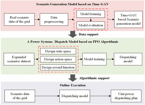
FIGURE 1. Framework of data-driven dispatch with scenario generation.

3 Time-GAN-based scenario generation

Based on the framework of data-driven dispatch with scenario generation in Section 1, a Time-GAN-based scenario generation model is constructed in this section. A scenario generation model based on Time-GAN is constructed to solve the problem of insufficient samples in data-driven models. It provides data support for the data driven distribution model in Section 3.

3.1 Scenario generation

The scenario generation process based on Time-GAN is shown in Figure 2, which is mainly divided into the following four steps.

(a) Preprocessing real scenarios. To obtain the distribution features of the data, the real scenarios obtained are subjected to data cleaning and normalization.

(b) Training Time-GAN for scenario generation. The Time-GAN parameters are set, including the sampling time step, the maximum training step, the hyperparameter, and batch size, and training the Time-GAN model.

(c) Generating renewable energy generation and load scenarios. The trained scenario generation network and test data are utilized for scenario generation.

(d) Evaluating the quality of scenario generation. The distribution features and spatiotemporal correlation of the generated scenarios are evaluated.

FIGURE 2

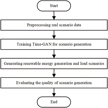
FIGURE 2. Flow of scenario generation based on Time-GAN.

3.2 Scenario generation based on Time-GAN

For Time-GAN, while preserving the structure of the generator and discriminator of GAN, AEN was added for joint training to achieve adversarial and supervised training, enabling the model to learn time-series data that conform to the feature distribution of the real data, as shown in Figure 3.

FIGURE 3

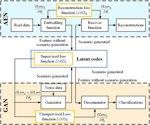
FIGURE 3. Time-GAN model structure.

First, $S$ is defined as the static feature vector, representing renewable energy or load data at a certain time. Furthermore, $X$ is defined as the dynamic feature vector, representing renewable energy or load data at a certain node at a certain period, and it is the variable information in the scenarios. We assume $\left(S,X_{1:T}\right)$ follows a certain joint distribution $p$, where $T$ is the length of the time series. The training sample set is $={\left\{\left(S^n,X_{1:T}^n\right)\right\}}_{n=1}^N$, and $n=\left(1,\dots ,N\right)$ is the $n$-th training sample; the total number is $N$.

Second, the real scenarios obtained will be used as the training set, and it will be normalized as follows:

$x_t^{*}=\frac{x_t-x_{\mathit{min}}}{x_{\mathit{max}}-x_{\mathit{min}}},(1)$

where $x_t$ is the value at time $t$; $x_t^{*}$ is the normalized value at time $t$; and $x_{\mathit{max}}$ and $x_{\mathit{min}}$ are the maximum and minimum values of the sample before normalization, respectively.

Third, the real data on renewable energy or load containing both static and dynamic features are reconstructed in the autoencoder. The embedding function and recover function are given as follows:

$\left\{\begin{array}{c}{H}_s=E_s\left(S\right)\\ H_t=E_t\left(H_s,H_{t-1},X_t\right),\end{array}\right.(\mathrm{2a})$

$\left\{\begin{array}{c}\stackrel{\sim }{S}=R_s\left(H_s\right)\\ {\stackrel{\sim }{X}}_t=R_t\left(H_t\right),\end{array}\right.(\mathrm{2b})$

where (2. a) maps $S$ to a low-dimensional feature vector. Thus, the key feature vector is obtained, which is the latent encoding. Moreover, by (2.b), the low-dimensional vector is restored to the real high-dimensional vector. $H_s$ is the low-dimensional static feature vector after embedding function mapping; $H_t$ is the low-dimensional dynamic feature vector at time $t$ after passing through the embedded function; $X_t$ is the real high-dimensional dynamic feature vector at time $t$; $\stackrel{\sim }{S}$ and ${\stackrel{\sim }{X}}_t$ are the high-dimensional static and dynamic feature vectors recovered by the recovery function, respectively; and $E$ and $R$ are embedding functions and reconstruction functions, respectively. To optimize AEN, the loss function ${Loss}_R$ of AEN is expressed as follows:

${Loss}_R=E_{S,X_{1:T\sim p}}\left[{‖S-\stackrel{\sim }{S}‖}_2+{\displaystyle {\sum }_t}{‖X_t-{\stackrel{\sim }{X}}_t‖}_2\right].(3)$

Meanwhile, the discriminator is used to determine whether the generated data are similar to the real data. The generator and discriminator are given as follows:

$\left\{\begin{array}{c}{\widehat{H}}_s=G_s\left(Z_S\right)\\ {\widehat{H}}_t=G_t\left({\widehat{H}}_s,{\widehat{H}}_{t-1},Z_t\right),\end{array}\right.(\mathrm{4a})$

$\left\{\begin{array}{c}{\widehat{y}}_S=D_s\left({\widehat{H}}_s\right)\\ {\widehat{y}}_t=D_t\left({\widehat{U}}_t,X_t\right),\end{array}\right.(\mathrm{4b})$

where ${\widehat{H}}_s$ and ${\widehat{H}}_t$ are static and dynamic feature vectors generated, respectively. ${\widehat{y}}_S$ and ${\widehat{y}}_t$ are the classification results generated by static and dynamic features, respectively. ${\widehat{U}}_t$ is the joint encoding output result; and $G$ and $D$ are generator and discriminator functions, respectively. To improve Time-GAN, the joint loss function ${Loss}_E$ of the generator and discriminator is given as follows:

${Loss}_E={Loss}_G+{Loss}_D,(\mathrm{5a})$

$\left\{\begin{array}{c}{Loss}_G=E_{S,X_{1:T\sim \widehat{p}}}\left[\log \left(1-{\widehat{y}}_S\right)+{\displaystyle {\sum }_t}\left(1-\mathit{log}{\widehat{y}}_t\right)\right]\\ {Loss}_D=E_{S,X_{1:T\sim p}}\left[\mathit{log}{y}_S+{\displaystyle {\sum }_t}\mathit{log}{y}_t\right],\end{array}\right.(\mathrm{5b})$

where $y_S$ and $y_t$ are the classification results of the original dynamic and static feature data, respectively.

Finally, defining the supervised loss function ${Loss}_S$ between the generator and the real data evaluates the time-series correlation learning ability of the generator as follows:

${Loss}_S=E_{S,X_{1:T\sim p}}\left[{\displaystyle {\sum }_t}{‖H_t-G_s\left(H_s,H_{t-1},Z_t\right)‖}_2\right].(6)$

3.3 Scenario generation quality assessment

To verify the effectiveness of the scenario generation model based on Time-GAN, this paper uses t-SNE (Wang et al., 2022) to evaluate the data distribution features, the autocorrelation coefficient method (Chen et al., 2018) to evaluate time-series correlation, and the Pearson method (Burgund et al., 2023) to evaluate spatial correlation.

(a) Data distribution feature evaluation based on t-SNE. t-SNE can display clear boundaries in low-dimensional space while preserving the original information on the data, making the visualization results more intuitive. Therefore, t-SNE is used to evaluate the effectiveness of the scenario generation model based on Time-GAN in this paper. The algorithm steps are listed as follows:

1) In a high-dimensional space, assume $x_i$ is the clustering center. The probability $P_{j|i}$ of other samples $x_j$ in this category is measured by the Gaussian probability density function as follows:

$P_{j|i}=\frac{\exp \left(-\frac{{‖x_i-x_j‖}^2}{2{\sigma }_i^2}\right)}{{\displaystyle {\sum }_{k\ne i}}\exp \left(-\frac{{‖x_i-x_j‖}^2}{2{\sigma }_i^2}\right)},(\mathrm{7a})$

$P_{i|j}=\frac{P_{i|j}+P_{j|i}}{2K},(\mathrm{7b})$

where $x_i$ and $x_j$ are high-dimensional data; ${\sigma }_i$ is the variance of the Gaussian distribution; and $K$ is the total number of data points.

2) In a low-dimensional space, the low-dimensional representation of $x_i$ is $y_i$, and the low-dimensional representation of $x_j$ is $y_j$. Assuming $y_i$ is the cluster center, the probability of other data points $y_j$ belonging to this class $Q_{i|j}$ is measured using the t-distribution function:

$Q_{i|j}=\frac{{\left(1+{‖y_i-y_j‖}^2\right)}^{-1}}{{\displaystyle \sum _{k\ne i}}{\left(1+{‖y_i-y_j‖}^2\right)}^{-1}}.(8)$

3) The cost function $C$ can be obtained using the KL distance, and the visualization results of high-dimensional data can be obtained as follows:

$C=KL\left(P‖Q\right)={\sum }_i{\sum }_j{P}_{j|i}\mathit{log}\frac{P_{j|i}}{Q_{i|j}},(9)$

where $P$ and $Q$ are the joint probability distribution of samples in high-dimensional and low-dimensional spaces, respectively.

(b) Time-series correlation evaluation based on the autocorrelation coefficient method. The autocorrelation coefficient represents the correlation between moments, which can provide a very intuitive understanding of the relationship between time-series variables. Therefore, the autocorrelation coefficient method is used to analyze the time-series correlation of scenarios. The autocorrelation coefficient of scenarios is given as follows:

$F={\displaystyle {\sum }_{i=1}^{n-h}}\frac{\left(x_i-\overline{x}\right)\left(x_{i+h}-\overline{x}\right)}{{\displaystyle {\sum }_{i=1}^n}{\left(x_i-\overline{x}\right)}^2},(10)$

where $x_i$ is the $i$-th value of set $x$, $\overline{x}$ is the mean of the overall sample $x$, and $i=1,\dots ,n-h$.

(c) Spatial correlation evaluation based on the Pearson coefficient method. The advantage of using the Pearson coefficient method to evaluate the correlation of spatial sequences is that it can quickly measure the degree of correlation between two spatial sequences, to better understand the relationship between scenarios. The spatial correlation of scenarios is analyzed using the Pearson method; the Pearson coefficient of scenarios is expressed as follows:

$\rho =\frac{E\left[\left(x-\overline{x}\right)\left(y-\overline{y}\right)\right]}{\sqrt{{\displaystyle {\sum }_{i=1}^n}{\left(x_i-\overline{x}\right)}^2}\sqrt{{\displaystyle {\sum }_{i=1}^n}{\left(y_i-\overline{y}\right)}^2}},(11)$

where $x_i$ and $y_i$ are the $i$-th values of $x$ and $y$, respectively. $\overline{x}$ and $\overline{y}$ are the mean values of the sets $x$ and $y$, respectively, and $i=1,\dots ,n$.

4 Data-driven dispatch model considering “N-1” security

The high proportion of renewable energy penetration significantly enhances the uncertainty of the power system, and multiple energy sources bring strong coupling and non-linearity. It results in difficultly for traditional methods to model and achieve rapid optimization solutions. RL can enhance decision-making and reduce dependence on physical modeling. Therefore, based on scenario generation in the previous section, a data-driven dispatch model was constructed, which is implemented by the RL algorithm.

4.1 Model formulation

4.1.1 Objective

The objective function includes minimizing the total operating cost of the units and maximizing the consumption of renewable energy.

1) Operating cost objective is given as follows:

$F1=\mathit{min}{\displaystyle {\sum }_{i=1}^N}{\displaystyle {\sum }_{t=1}^T}\left(F_{it}\left(P_{it}\right)*U_{it}\right),(12)$

where $F_{it}\left(P_{it}\right)=a_i+b_i*P_{it}+c_i*P_{it}^2$, and $a_i$, $b_i$, and $c_i$ are, respectively, the constant term, primary term, and secondary term coefficients of the operating cost of the $i$-th unit. $P_{it}$ is the unit output of the $i$-th unit at time $t$; $U_{it}$ is the starting and stopping statuses of the $i$-th unit at time $t$; $N$ is the number of units; and $T$ is the operating time of the unit.

2) Renewable energy consumption objective is given as follows:

$F2=\mathit{max}\frac{{\displaystyle {\sum }_{i=1}^{Nr}}{\displaystyle {\sum }_{t=1}^{Tr}}{P}_{\mathrm{N}it}}{{\displaystyle {\sum }_{i=1}^{Nr}}{\displaystyle {\sum }_{t=1}^{Tr}}{P}_{\mathrm{N}it}^{\mathit{max}}},(13)$

where $P_{\mathrm{N}it}$ and $P_{Nit}^{\mathit{max}}$ are the actual and maximum output power of the $i$-th renewable energy unit at time $t$, respectively; and $Nr$ and $Tr$ are the number and operating time of the renewable energy unit, respectively.

4.1.2 Constraints

1) The alternating current power flow constraint is given as follows:

$\left\{\begin{array}{c}{P}_{it}-P_{\mathrm{L}it}=V_{it}{\displaystyle {\sum }_{j=1}^n}{V}_{jt}\left(G_{ij}\mathit{cos}{\delta }_{ijt}+B_{ij}\mathit{sin}{\delta }_{ijt}\right)\\ Q_{it}-Q_{\mathrm{L}it}=V_{it}{\displaystyle {\sum }_{j=1}^n}{V}_{jt}\left(G_{ij}\mathit{sin}{\delta }_{ijt}-B_{ij}\mathit{cos}{\delta }_{ijt}\right),\end{array}\right.(14)$

where $P_{it}$ and $Q_{it}$ are the active and reactive power of the $i$-th unit at time $t$, respectively; $P_{\mathrm{L}it}$ and $Q_{Lit}$ are the active and reactive power of the $i$-th unit during the $t$-th period, respectively; $V_{it}$ is the voltage modulus of the $i$-th node; ${\delta }_{it}$ is the phase angle difference between two nodes; and $G_{ij}$ and $B_{ij}$ are the conductivity and admittance between nodes $i$ and $j$, respectively.

2) The unit generating capacity constraint is given as follows:

${P_{Tit}^{\mathit{min}}*U_{it}\le P}_{Tit}\le P_{Tit}^{\mathit{max}}*U_{it},(15)$

where $P_{Tit}^{\mathit{min}}$ and $P_{Tit}^{\mathit{max}}$ are the generating capacity down and up limits of the $i$-th thermal unit at time $t$, respectively; and $P_{Tit}$ is the actual out power of the $i$-th thermal unit at time $t$.

3) The renewable energy generating capacity constraint is given as follows:

$P_{\mathrm{N}it}\le P_{\mathrm{N}it}^{\mathit{max}}*U_{it}.(16)$

4) The unit operating ramping constraint is given as follows:

$P_{Tit}^{\mathit{min}}*r\le P_{Tit}-P_{Ti\left(t-1\right)}\le P_{Tit}^{\mathit{max}}*r,(17)$

where $r$ is the operating ramping rate of the unit $P_{Tit}$.

5) The swing-bus unit generating capacity constraint is given as follows:

After the power flow calculation, the output power of the swing-bus unit is less than 110% of the up limit or greater than 90% of the down limit.

$P_{Bit}^{\mathit{min}}*0.9\le P_{Bit}\le P_{Bit}^{\mathit{max}}*1.1,(18)$

where $P_{Bit}$ is the output power of the $i$-th swing-bus unit at time $t$; $P_{Bit}^{\mathit{min}}$ and $P_{Bit}^{\mathit{max}}$ are the generating capacity down and up limits of the $i$-th swing-bus unit at time $t$, respectively.

6) “N-1” security constraint is given as follows:

In this paper, the operational risk of the power system “N-1” is considered. The voltage of adjacent nodes with line disconnection can neither be greater than the up limit of the voltage of that node nor can it be less than the lower limit of the voltage of that node.

$\left\{\begin{array}{l}{V}_i^{\mathit{min}}\le V_i\le V_i^{\mathit{max}}\\ V_j^{\mathit{min}}\le V_j\le V_j^{\mathit{max}},\end{array}\right.(19)$

where $V_i$ and $V_j$ are the node voltages at both ends of line ${\mathrm{L}}_{ij}$, respectively; and $V_i^{\mathit{min}}$ and $V_j^{\mathit{min}}$ are the down and up limits of node voltages at both ends of line ${\mathrm{L}}_{ij}$, respectively.

4.2 Solution based on the RL algorithm

The aforementioned dispatch problem would be transformed into a RL power system dispatch model based on the data-driven approach, specifically including the design of state space, action space, and reward function.

4.2.1 State space

The information that can be obtained by the agent in actual environments will be considered due to the limitations of physical communication systems and data privacy. The influence of the large-scale state space on model convergence speed is also considered. The agent obtains the state space $S_t$ at time $t$ is set to

$S_t=\left\{P_t,P_{\mathrm{L}t},P_{t+1},P_{\mathrm{L}t+1},P_{\mathrm{N}t}^{\mathit{max}},V_t\right\},(20)$

where $P_t$ is the output power of the unit at time $t$; $P_{\mathrm{L}t}$ is the load of each node at time $t$; $P_{t+1}$ is output power of the unit at time $t+1$; $P_{\mathrm{L}t+1}$ is the load of each node at time $t+1$; $P_{Nt}^{\mathit{max}}$ is the predicted maximum output power of the renewable energy unit at time $t$; and $V_t$ is the node voltages at time $t$.

4.2.2 Action space

In the dispatch model based on RL, the output of the agent at time $t$ is $P_{it}$. $A_t$ is the action of the agent at time $t$. The joint action at the time $t$ is expressed as follows:

$A_t=\left\{P_{1t},P_{2t},\dots ,P_{it}\right\}.(21)$

4.2.3 Reward function

Reward function used to describe environmental evaluation agent action $A_t$. The reward functions are set:

1) Reward function for line power exceeding limit is expressed as follows:

$r_{1t}=\frac{1}{n_{line}}{\displaystyle {\sum }_{l=1}^{n_{line}}}r{ho}_{lt},(22)$

where $n_{line}$ is the number of power grid branches and $r{ho}_{lt}$ is the current load rate of branch $l$ at time $t.$

2) Reward function for renewable energy consumption is expressed as follows:

$r_{2t}=\frac{{\displaystyle {\sum }_{i=1}^{Nr}}{P}_{\mathrm{N}it}}{{\displaystyle {\sum }_{i=1}^{Nr}}{P}_{Nit}^{\mathit{max}}}.(23)$

3) Reward function for swing-bus units exceeding limit is expressed as follows:

$r_{3t}=-{\displaystyle {\sum }_{i=1}^{n_{balanced}}}\Delta P_{\mathrm{B}it},(\mathrm{24a})$

$\Delta P_{Bit}=\left\{\begin{array}{cc}\left|\frac{P_{\mathrm{B}it}-P_{Bit}^{\mathit{max}}}{P_{Bit}^{\mathit{max}}}\right|& P_{Bit}^{\mathit{max}}<P_{Bit}<1.1*P_{Bit}^{\mathit{max}}\\ \left|\frac{P_{Bit}-P_{Bit}^{\mathit{max}}}{P_{Bit}^{\mathit{max}}}\right|& 0.9*P_{Bit}^{\mathit{max}}<P_{Bit}<P_{Bit}^{\mathit{max}}\\ 0& \text{others},\end{array}\right.(\mathrm{25b})$

where $n_{balanced}$ is the number of swing-bus units.

4) The unit operating cost reward function is expressed as follows:

$r_{4t}=-{\displaystyle {\sum }_{i=1}^N}\left(a_i+b_i*P_{it}+c_i*P_{it}^2\right)U_{it}.(26)$

5) Reward function for line node voltage exceeding limit is expressed as follows:

$r_{5t}=-{\displaystyle {\sum }_{i=1}^{n_{sub}}}\Delta V_i,(\mathrm{27a})$

$\Delta V_i=\left\{\begin{array}{cc}\left|\frac{V_i-V_i^{\mathit{max}}}{V_i^{\mathit{max}}}\right|& V_i>V_i^{\mathit{max}}\\ \left|\frac{V_i-V_i^{\mathit{min}}}{V_i^{\mathit{min}}}\right|& V_i<V_i^{\mathit{max}}\\ 0& \text{others},\end{array}\right.(\mathrm{27b})$

where $n_{sub}$ is the number of nodes.

The reward functions $r_{3\mathrm{t}}$, $r_{4\mathrm{t}}$, and $r_{5\mathrm{t}}$ are normalized:

$r=e^r-1.(28)$

In summary, the domain values of $r_{1\mathrm{t}}$, $r_{2\mathrm{t}}$, and $r_{5t}$ are $\left[0,1\right]$, while the domain values of $r_{3\mathrm{t}}$ and $r_{4\mathrm{t}}$ are $\left[-1,0\right]$. The total reward functions are given as follows:

$R_t={\alpha }_1{r}_{1t}+{\alpha }_2{r}_{2t}+{\alpha }_3{r}_{3t}+{\alpha }_4{r}_{4t}+{\alpha }_5{r}_{5t},(29)$

where $r_{it}$ is the $i$-th reward function at time $t$; ${\alpha }_i$ is the coefficient of the $i$-th reward function; $i=\mathrm{1,2},\dots ,5$.

5 Offline training and online execution

Based on the scenario generation model in Section 2 and the dispatch model in Section 3, the process of offline training and online execution of the dispatch model is discussed in this section and shown in Figure 4.

FIGURE 4

FIGURE 4. Offline training and online execution process.

5.1 Offline training process

Compared to other RL methods, the PPO algorithm adopts important sampling technology to effectively utilize historical data, avoiding the problem of large variance and being able to handle the problem of continuous action space. So the PPO algorithm is chosen to study the power system dispatch problem.

First, the policy network and value network make actions $A_t$ and calculate the value function $V_{\mu }\left(S_t\right)$ based on $S_t$, respectively. Then, $A_t$ is input into the environment, and the action reward $R_t$ and the new environment state $S_{t+1}$ are obtained. Finally, the sample data $\left(S_t,A_t,R_t,S_{t+1}\right)$ are stored in the sample batches (Huang and Wang, 2020).

For value network updates, $\left(S_t,A_t,R_t,S_{t+1}\right)$ is obtained from the sample batches, and $V_{\mu }\left(S_t\right)$ is calculated. According to the loss function (31) and gradient function (30), the value network is gradient-updated.

$\mu =\mu -l_{\mu }\nabla L^V\left(\mu \right),(30)$

$L^V\left(\mu \right)=E{\left(R_t+\gamma V_{\mu }\left(S_{t+1}\right)-V_{\mu }\left(S_t\right)\right)}^2,(31)$

where $\mu$ and $l_{\mu }$ are the parameter and learning rate of the value network, respectively; $\nabla L^V\left(\mu \right)$ is the gradient of value network loss function $L^V\left(\mu \right)$ with respect to $\mu$; and $E\left(·\right)$ is the expectation.

Unlike the parameter update of the value network, the performance of the policy network is improved according to the advantage function $\widehat{A}\left(S_t,A_t\right)$ (Chen et al., 2023b). The parameter update formula of the policy network is given as follows:

$\theta =\theta -l_{\theta }\nabla \widehat{A,}(32)$

$\widehat{A}\left(S_t,A_t\right)=Q_{\mu }\left(S_t,A_t\right)-V_{\mu }\left(S_t\right),(33)$

$\left\{\begin{array}{c}{Q}_{\mu }\left(S_t,A_t\right)=E\left(R_t|S_t,A_t;\pi \right)\\ V_{\mu }\left(S_t\right)=E\left(R_t|S_t;\pi \right),\end{array}\right.(34)$

where $\theta$ and $l_{\theta }$ are the parameter and learning rate of the policy network, respectively; $\nabla \widehat{A}$ is the gradient of the loss function $\widehat{A}$ of the policy network with respect to $\theta$; $Q_{\mu }\left(S_t,A_t\right)$ is the expected reward value of $A_t$ based on policy $\pi$ in $S_t$, which is the action value function; and $V_{\mu }\left(S_t\right)$ is the expected reward value obtained by taking all possible actions according to $\pi$ in $S_t$, which is the state value function. To improve the training speed, a parallel training method is adopted to train the PPO algorithm.

5.2 Online execution process

As shown in Figure 4, in the online execution process, the dispatch policy of the power system only relies on the trained policy network and does not require the participation of the value network. When the dispatch task arrives, the dispatch action $A_t$ is made based on $S_t$ by the agent, and the environment executes this action and transfers to the next state $S_{t+1}$, while the reward value $R_t$ is calculated. Then, The load demand and environmental status are continued to be collected at the next moment until the execution process for the total $T$ period is completed.

6 Simulation

The environment is constructed based on a real power system in a province in south China, which includes 748 nodes, 845 branches, and 187 units (55 renewable energy generation, 131 thermal units, and 1 swing-bus unit). The dispatch interval is 15 min. The sampling time step in Time-GAN is 96, the maximum training step is 35,000, the hyperparameter $\mathrm{\gamma }$ is 1, and the batch size is 32. In RL, the learning rate is 10^–5, the maximum training episode is 10⁷, and the number of parallel environments is 88; the mini-batch is 128. All simulations are based on Python 3.6 and PyTorch 1.6.

6.1 Scenario generation example analysis

The aforementioned grid structure historical scenario is used to build a scenario generation model based on Time-GAN, and the scenario generation effect of the model is verified. The real scenario contains 2000 scenario section data, and the ratio of training and testing scenarios is 4:1.

(a) Analysis of the distribution of scenario generation. To test the performance of the algorithm, the scenarios generated by Time-GAN and Time-VAE were compared and analyzed. The feature distribution between the generated scenarios and the real scenarios was visualized using t-NSE, as shown in Figure 5. It can be seen that the feature distribution of Time-VAE-generated scenarios is significantly different from that of the real scenarios, and a large number of scenarios that deviate from the distribution features of the real scenarios were generated. It indicates that its effectiveness in generating scenarios is not high. The feature distribution of scenarios generated by Time-GAN is relatively close to that of real scenarios, fitting the feature distribution of the real scenarios. It indicates that Time-GAN is more effective in generating scenarios than Time-VAE.

(b) Analysis of scenario time-series correlation features based on the autocorrelation coefficient. To study the correlation between generated scenarios and real scenarios in terms of time-series correlation features, autocorrelation coefficients are introduced. The autocorrelation coefficients of scenarios are shown in Figure 6. Within the lag range of 0–20 h, the autocorrelation coefficients of the generated renewable energy and the real scenarios are consistent. This indicates that the generated scenarios can accurately simulate and preserve the correlation features of time series in real scenarios. The long-time scale time-series correlation features of the generated scenarios meet the requirements of the time-series correlation features of the real scenarios.

(c) Analysis of the scenario spatial correlation based on the Pearson coefficient method. To study the correlation between generated scenarios and real scenarios in terms of spatial features, the Pearson coefficient method is introduced. The Pearson coefficient results of renewable energy and load are shown in Tables 1–4. It can be seen that the spatial correlation between the renewable energy and load scenarios generated by this method and real scenarios is relatively close. The overall generated scenarios comply with the correlation rule of real scenarios. This shows that the renewable energy and load scenario generation method in this paper can learn the complex coupling between renewable energy and loads, and has a good generalization effect.

FIGURE 5

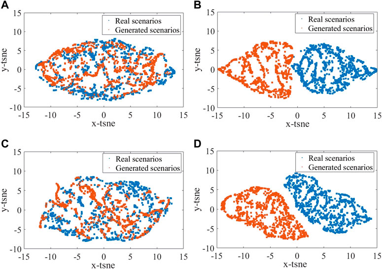
FIGURE 5. t-SNE visualization of Time-GAN-based renewable energy scenarios (A). Time-VAE-based renewable energy scenarios (B). Time-GAN-based load scenarios (C). Time-VAE-based load scenarios (D).

FIGURE 6

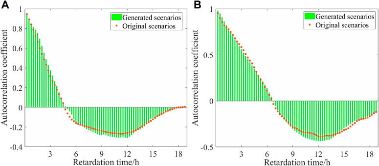
FIGURE 6. Autocorrelation coefficients of renewable energy scenarios (A) and load scenarios (B).

TABLE 1

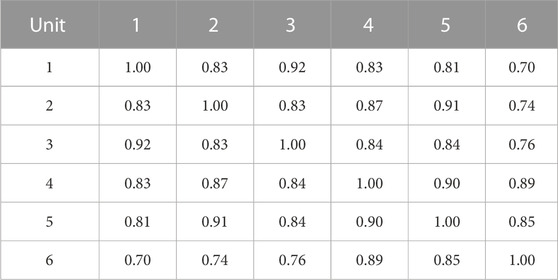
TABLE 1. Correlation of real renewable energy scenarios.

TABLE 2

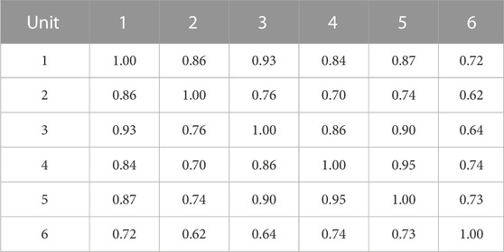
TABLE 2. Correlation of renewable energy scenarios generated.

TABLE 3

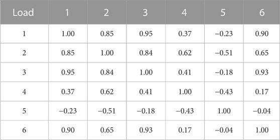
TABLE 3. Correlation of real load scenarios.

TABLE 4

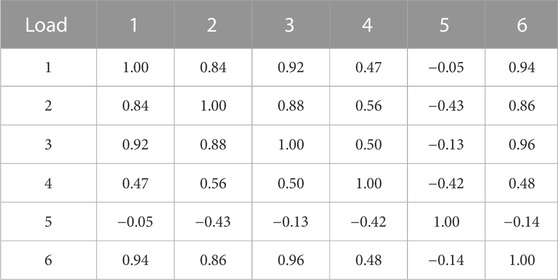
TABLE 4. Correlation of load scenarios generated.

6.2 Analysis of power system dispatch results

A data-driven power system dispatch model is constructed based on the aforementioned scenario generation. First, the original 2000 section scenarios are expanded to 10,000 section scenarios through the scenario generation model. Second, the dispatch model is training. Finally, the trained dispatch model was tested using actual real sample scenarios to verify its effectiveness.

6.2.1 Analysis of RL convergence

This paper not only compares the training effects of the dispatch model before and after scenario generation but also compares the PPO algorithm with other RL methods. The reward convergence of model training is shown in Figure 7. “O-PPO” represents the convergence curve of the PPO algorithm training based on real scenarios, and “G-PPO, G-A3C, G-A2C, G-DDPG, and G-APPO” represents the convergence curve of training based on scenario generation. From Figure 7, the following can be observed:

(a) Comparing the convergence curves of O-PPO and G-PPO, it can be seen that scenario generation can improve the training effect of the dispatch model based on the PPO algorithm. From the perspective of the average reward value, the overall training effect of G-PPO has improved by 607.49% compared to O-PPO. This means that by using scenarios generated by the scenario generation model for training, the data-driven dispatch model can be better optimized and its performance improved. A key advantage of using scenario generation models for training is that it can generate a large amount of rich and diverse scenario data, which expands the diversity of the training dataset. Due to the possible differences between the generated scenario data and the real scenario, the model can learn a wider range of situations and coping methods, thus possessing stronger generalization ability. This demonstrates the importance of scenario generation in improving the performance of the data-driven dispatch model.

(b) Comparing the convergence curves of G-PPO with other RL algorithms (G-A3C, G-A2C, G-DDPG, and G-APPO), it can be seen that the average reward convergence effect of the PPO algorithm is better. The dispatch model based on the PPO algorithm is more suitable for optimizing dispatch execution in this scenario.

FIGURE 7

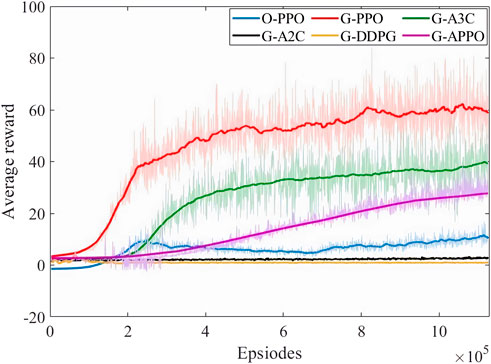
FIGURE 7. Curve of reward function during the training process.

6.2.2 Analysis of dispatch results

(a) Analysis of output power of units. A certain section is selected as the testing scenario, and the method proposed is used for real-time dispatch. The dispatch results are shown in Figure 8. In the time sections numbered 1–28, when output power of renewable energy is low, the method proposed achieves load demand by increasing the output of thermal power units in this paper. This method prioritizes using renewable energy to meet the load and reduce output power of thermal power units. In the time sections of 44–96, when output power of renewable energy is high, this method prioritizes using renewable energy to meet the load demand and reduce output power of thermal power units. In the time sections of 29–43, when the load demand and the renewable energy output power are low, this method makes a reasonable dispatch plan for output power of thermal power units to meet the load demand. At the same time, output power of the swing-bus unit is always maintained between 300 and 800 MW (the generating capacity up limit of the swing-bus unit is 878.9 MW), meeting the real-time safety regulation margin of the swing-bus unit.

(b) Analysis of the consumption of renewable energy. The consumption of renewable energy has always been a key issue in the operation and planning of the power system. The method proposed in this paper aims to achieve the actual output power of renewable energy as close as possible to its maximum power through reasonable dispatch of the system. The maximum power, actual output power, and consumption rate of renewable energy power are shown in Figure 9. In this paper, 100% renewable energy consumption cannot be guaranteed using the method proposed, but the overall renewable energy consumption rate reaches 94.06%. Based on Figure 8, it can be seen that a high level of renewable energy consumption can also be ensured during the large-scale development of renewable energy. This is of great significance for promoting the development of renewable energy and improving the sustainability of the power system.

(c) Analysis of node voltage exceeding the limit for “N-1”. At the same time, the aforementioned dispatch plan was verified using alternating current power flow through “N-1” safety verification, and the node voltage at different times under any fault was obtained, as shown in Figure 10. By comparing voltage values with the set safety range, it can be determined whether the system is experiencing abnormal or overload situations. From Figure 9, it is observed that the node voltage remains within a safe range, indicating that the dispatch scheme ensures the stability and safety of the power system under the “N-1” fault state. The power system dispatch plan based on RL can ensure the stability of node voltage in the event of a fault, which is crucial for the operation of the power system and thus ensures the reliable power supply of the power system.

(d) Comparative analysis with traditional methods. To further verify the rationality and effectiveness of the method proposed in this paper, the convex optimization problem (OPT) (Tejada-Arang et al., 2017) is used for comparative analysis, and the Gurobi solver was used for the solution. The comparison results of cross-section scenarios A and B are shown in Table 5. Due to the large scale of the optimization problem in this paper, although the training speed of the method in this paper is slow, the online solution time is reduced by more than 99% compared to traditional OPT methods. At the same time, neither the method proposed in this paper nor traditional OPT methods can fully guarantee 100% renewable energy consumption throughout the entire time period. However, compared to the OPT method, this method can also provide a higher level of the renewable energy consumption rate. In summary, the method proposed in this paper not only has fast dispatch decision-making speed but also can achieve high renewable energy consumption.

FIGURE 8

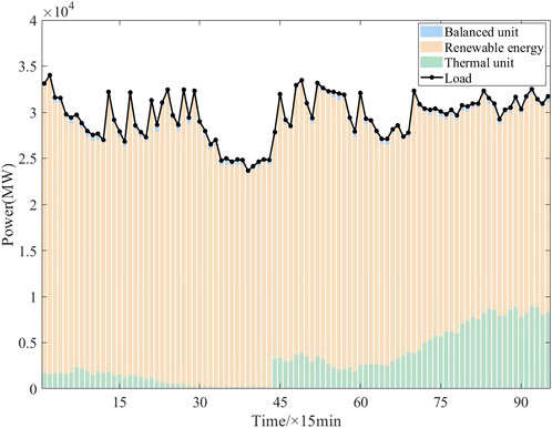
FIGURE 8. Dispatch results of units by the PPO algorithm.

FIGURE 9

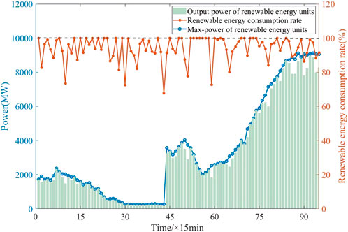
FIGURE 9. Output power and consumption rate of renewable energy.

FIGURE 10

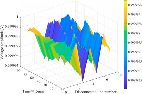
FIGURE 10. Node voltage under “N-1” faults.

TABLE 5

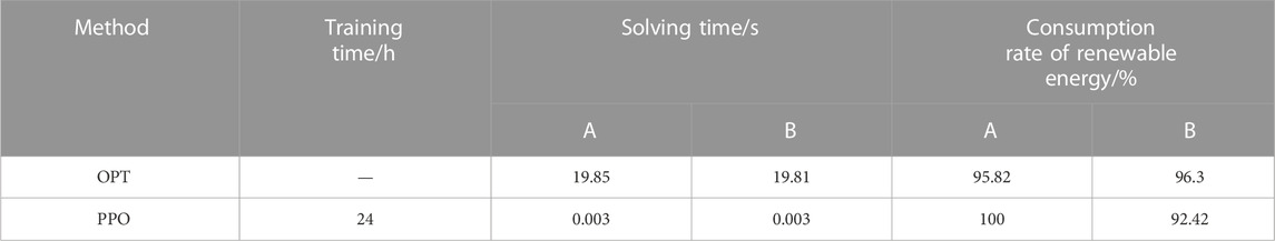
TABLE 5. Comparison of dispatch results under different methods.

7 Conclusion

To ensure the effectiveness of the data-driven dispatch under insufficient scenario samples, a data-driven dispatch method with time-series correlated scenario generation is proposed. The results verify that the performance can be effectively improved by scenario generation. The proposed dispatch model can bring significant economic benefits and renewable energy consumption. It can also ensure the security under “N-1″ contingencies. Compared with traditional optimization-based methods, the proposed method reduces the online solution time by more than 99%.

Future research can focus on the action of safety and interpretability issues when applying RL in power systems.

Data availability statement

The original contributions presented in the study are included in the article/Supplementary Material; further inquiries can be directed to the corresponding author.

Author contributions

PL: writing–review and editing, data curation, and investigation. WH: writing–review and editing, data curation, resources, and supervision. LL, ZD, and JH: writing–review and editing, investigation, and supervision. SC: writing–review and editing, formal analysis, and supervision. HZ: writing–review and editing, investigation, resources, and supervision. XZ: writing–review and editing and supervision. WM: conceptualization, methodology, software, and writing–original draft. LC: writing–review and editing, conceptualization, formal analysis, and supervision.

Funding

The author(s) declare financial support was received for the research, authorship, and/or publication of this article. This work is supported by the Science and Technology Project of China Southern Power Grid Digital Grid under grant number (670000KK52220002).

Conflict of interest

PL, WH, LL, ZD, SC, HZ, XZ, JH was employed by the Southern Power Grid Digital Grid Research Institute.

The remaining authors declare that the research was conducted in the absence of any commercial or financial relationships that could be construed as a potential conflict of interest.

The authors declare that this study received funding from the Science and Technology Project of China Southern Power Grid Digital Grid Research Institute [670000KK52220002]. The funder had the following involvement in the study: Study sponsor.

Publisher’s note

All claims expressed in this article are solely those of the authors and do not necessarily represent those of their affiliated organizations, or those of the publisher, the editors, and the reviewers. Any product that may be evaluated in this article, or claim that may be made by its manufacturer, is not guaranteed or endorsed by the publisher.

References

Bagheri, F., Dagdougui, H., and Gendreau, M. (2022). Stochastic optimization and scenario generation for peak load shaving in Smart District microgrid, sizing and operation. Energy Build. 275, 112426. doi:10.1016/j.enbuild.2022.112426

CrossRef Full Text | Google Scholar

Burgund, D., Nikolovski, S., Galić, D., and Maravić, N. (2023). Pearson correlation in determination of quality of current transformers. Sensors 23 (5), 2704. doi:10.3390/s23052704

PubMed Abstract | CrossRef Full Text | Google Scholar

Chen, H., Zhuang, J., Zhou, G., Wang, Y., Sun, Z., and Levron, Y. (2023b). Emergency load shedding strategy for high renewable energy penetrated power systems based on deep reinforcement learning. Energy Rep. 9, 434–443. doi:10.1016/j.egyr.2023.03.027

CrossRef Full Text | Google Scholar

Chen, Q., Lin, N., Bu, S., Wang, H., and Zhang, B. (2023a). Interpretable time-adaptive transient stability assessment based on dual-stage attention mechanism. IEEE Trans. Power Syst. 38 (3), 2776–2790. doi:10.1109/tpwrs.2022.3184981

CrossRef Full Text | Google Scholar

Chen, Y., Wang, Y., Kirschen, D., and Zhang, B. (2018). Model-free renewable scenario generation using generative adversarial networks. IEEE Trans. Power Syst. 33 (3), 3265–3275. doi:10.1109/tpwrs.2018.2794541

CrossRef Full Text | Google Scholar

Fraccaro, M., Sønderby, S. K., Paquet, U., et al. (2016). Sequential neural models with stochastic layers. Adv. neural Inf. Process. Syst., 2207–2215.

Google Scholar

Goh, H., Peng, G., Zhang, D., Dai, W., Kurniawan, T. A., Goh, K. C., et al. (2022). A new wind speed scenario generation method based on principal component and R-Vine copula theories. Energies 15 (7), 2698. doi:10.3390/en15072698

CrossRef Full Text | Google Scholar

Han, X., Mu, C., Yan, J., and Niu, Z. (2023). An autonomous control technology based on deep reinforcement learning for optimal active power dispatch. Int. J. Electr. Power & Energy Syst. 145, 108686. doi:10.1016/j.ijepes.2022.108686

CrossRef Full Text | Google Scholar

He, Y., Zang, C., Zeng, P., Dong, Q., Liu, D., and Liu, Y. (2023). Convolutional shrinkage neural networks based model-agnostic meta-learning for few-shot learning. Neural Process. Lett. 55 (1), 505–518. doi:10.1007/s11063-022-10894-7

CrossRef Full Text | Google Scholar

Huang, B., and Wang, J. (2020). Deep-reinforcement-learning-based capacity scheduling for PV-battery storage system. IEEE Trans. Smart Grid 12 (3), 2272–2283. doi:10.1109/tsg.2020.3047890

CrossRef Full Text | Google Scholar

Huang, Y., Li, P., Zhang, X., Mu, B., Mao, X., and Li, Z. (2021). A power dispatch optimization method to enhance the resilience of renewable energy penetrated power networks. Front. Phys. 9, 743670. doi:10.3389/fphy.2021.743670

CrossRef Full Text | Google Scholar

Irena, (2023). The cost of financing for renewable power. https://www.irena.org/Publications/2023/May/The-cost-of-financing-for-renewable-power.

Google Scholar

Jang, M., Jeong, H. C., Kim, T., and Joo, S. K. (2021). Load profile-based residential customer segmentation for analyzing customer preferred time-of-use (TOU) tariffs. Energies 14 (19), 6130. doi:10.3390/en14196130

CrossRef Full Text | Google Scholar

Ji, X., Li, Y., Yu, Y., and Fan, S. (2018). Optimal dispatching and game analysis of power grid considering demand response and pumped storage. Syst. Sci. Control Eng. 6 (3), 270–277. doi:10.1080/21642583.2018.1553074

CrossRef Full Text | Google Scholar

Krishna, A. B., and Abhyankar, A. R. (2023). Time-coupled day-ahead wind power scenario generation, A combined regular vine copula and variance reduction method. Energy 265, 126173. doi:10.1016/j.energy.2022.126173

CrossRef Full Text | Google Scholar

López-Garza, E., Domínguez-Cruz, R. F., Martell-Chávez, F., and Salgado-Tránsito, I. (2022). Fuzzy logic and linear programming-based power grid-enhanced economical dispatch for sustainable and stable grid operation in eastern Mexico. Energies 15 (11), 4069. doi:10.3390/en15114069

CrossRef Full Text | Google Scholar

Luo, J., Zhang, W., Wang, H., Wei, W., and He, J. (2023). Research on data-driven optimal scheduling of power system. Energies 16 (6), 2926. doi:10.3390/en16062926

CrossRef Full Text | Google Scholar

Qian, T., Shi, F., Wang, K., Yang, S., Geng, J., Li, Y., et al. (2022). N-1 static security assessment method for power grids with high penetration rate of renewable energy generation. Electr. Power Syst. Res. 211, 108200. doi:10.1016/j.epsr.2022.108200

CrossRef Full Text | Google Scholar

Seo, M., Vecchietti, L. F., Lee, S., and Har, D. (2019). Rewards prediction-based credit assignment for reinforcement learning with sparse binary rewards. IEEE Access 7, 118776–118791. doi:10.1109/access.2019.2936863

CrossRef Full Text | Google Scholar

Tang, H., Lv, K., Bak-Jensen, B., Pillai, J. R., and Wang, Z. (2022). Deep neural network-based hierarchical learning method for dispatch control of multi-regional power grid. Neural Comput. Appl. 34, 5063–5079. doi:10.1007/s00521-021-06008-4

CrossRef Full Text | Google Scholar

Tang, J., Liu, J., Wu, J., Jin, G., Kang, H., Zhang, Z., et al. (2023). RAC-GAN-based scenario generation for newly built wind farm. Energies 16 (5), 2447. doi:10.3390/en16052447

CrossRef Full Text | Google Scholar

Tejada-Arango, D. A., Sánchez-Martın, P., and Ramos, A. (2017). Security constrained unit commitment using line outage distribution factors. IEEE Trans. power Syst. 33 (1), 329–337. doi:10.1109/tpwrs.2017.2686701

CrossRef Full Text | Google Scholar

Wang, H., and Ouyang, Y. (2022). Adaptive data recovery model for PMU data based on SDAE in transient stability assessment. IEEE Trans. Instrum. Meas. 71, 1–11. doi:10.1109/tim.2022.3212551

CrossRef Full Text | Google Scholar

Wang, L., Tian, T., Xu, H., and Tong, H. (2022). Short-term power load forecasting model based on t-SNE dimension reduction visualization analysis, VMD and LSSVM improved with chaotic sparrow search algorithm optimization. J. Electr. Eng. Technol. 17 (5), 2675–2691. doi:10.1007/s42835-022-01101-7

CrossRef Full Text | Google Scholar

Wei, T., Chu, X., Yang, D., and Ma, H. (2022). Power balance control of RES integrated power system by deep reinforcement learning with optimized utilization rate of renewable energy. Energy Rep. 8, 544–553. doi:10.1016/j.egyr.2022.02.221

CrossRef Full Text | Google Scholar

Yang, J., Zhang, J., and Wang, H. (2020). Urban traffic control in software defined internet of things via a multi-agent deep reinforcement learning approach. IEEE Trans. Intelligent Transp. Syst. 22 (6), 3742–3754. doi:10.1109/tits.2020.3023788

CrossRef Full Text | Google Scholar

Yoon, J., Jarrett, D., and Van der Schaar, M. (2019). “Time-series generative adversarial networks,” in Proceedings of the 33rd International Conference on Neural Information Processing Systems, Vancouver, Canada, December, 2019, 5508–5518.

Google Scholar