Research on the identification of high-resistance ground faults in the flexible DC distribution network based on VMD–inception–CNN

With the rapid development of flexible DC distribution networks, fault detection and identification have also attracted people’s attention. High-resistance grounding fault poses a great challenge to the distribution network. The fault current is very small and random, which makes its detection and identification difficult. The traditional overcurrent protection device cannot identify and act on the fault current. Therefore, this paper proposes a fault detection method based on variational mode decomposition (VMD) combined with the convolutional neural network (CNN) of the inception module. This method first uses VMD to decompose the positive transient voltage. Second, it inputs the decomposed signal into CNN for training to obtain the optimal parameters of the model. Finally, the model performance is tested based on the PSCAD/EMTDC simulation platform. Experiments show that the detection method is accurate and effective. It can realize the accurate identification of seven different fault types.

1 Introduction

The AC distribution network faces problems such as tight power supply corridor and poor power quality. In recent years, medium-low voltage flexible DC distribution networks are widely used in power systems, which have the advantages of small line loss, large transmission capacity, and flexible operation mode. However, like the AC distribution network, high-resistance grounding faults are prone to occur due to the complex operating environment. The characteristics of faults are weak, thus making their detection impossible using common fault detection techniques (Silva et al., 2018). If they run for a long time, they will damage the wire insulation and pose a great threat to personal safety (Taheri and Razavi, 2018). On the other hand, the other faults and normal disturbances in the distribution network can also cause changes in voltage and current, causing difficulties in detection and identification. Therefore, how to accurately identify the faults is the focus of DC distribution network operation.

1.1 Previous and related work

At present, ground fault detection often uses signal processing methods. The collected signal usually includes voltage, current, magnetic field strength, and impedance. The commonly used signal decomposition methods are Fourier transform (FFT), empirical mode decomposition (EMD), and wavelet transform (WT). The Fourier transform can transform a continuous signal with a non-periodic time domain into a continuous signal with a non-periodic frequency domain. However, this method can only extract the information of the signal in the frequency component and is only applicable to non-stationary signals (Liu, 2022). EMD is a time-frequency processing method, which can reflect the local characteristics of non-stationary signals; however, the phenomenon of modal confusion occurs (Robertas et al., 2017). Adaptive noise-complete ensemble empirical mode decomposition mitigates the phenomenon of modal aliasing by adding Gaussian white noise to the signal to be processed; however, it does not make the phenomenon disappear completely and the added noise causes some interference (Xu et al., 2021). WT has advantages of processing non-stationary signals but requires artificial selection of the mother wavelet (Sarwagya and Ranjan, 2020). Gautam and Brahma (2013) used mathematical morphology-based methods that rely on irregularities in the current waveforms as HIF inception features. Satpathi et al. (2018) used short-time Fourier transform to quantitatively study high-frequency components under transient conditions and were able to distinguish between short-circuit faults and transient cases of sudden load changes. Song et al. (2022) used Minkowski distance measurement to measure the correlation of wave impedance and construct a fault detection scheme. Yao et al. (2019) proposed a feature extraction algorithm to extract scales with the essential fault features and determined the coefficient of the selected scale signal. Routray et al. (2015) presented a novel S-transform-based approach to detect the high-impedance fault in the distribution line. Xiang et al. (2019) extracted the high-frequency components in transient voltages by wavelet transform and proposed a fault identification method based on the difference of square of transient voltages to identify the fault lines for DC grids using overhead lines. Song et al. (2021) used the Hilbert–Huang transform to extract the transient frequency and transient amplitude of the DC voltage. The aforementioned signal extraction methods face some problems, such as the need to construct criteria manually and the lack of effective distinction between other types of faults and normal interference. Reliability needs to be further improved.

With the sudden rise in the scale of power grid data and the significant increase in computing power, the artificial neural network intelligent algorithm shows great superiority. With the enhancement of network depth, data dimension reduction and processing capability are further improved. It can extract useful information for fault identification accurately and effectively under the influence of complex external and internal environments. Chopdar and Koshti (2022) extracted fault feature signals using wavelet transform and trained these signals using the artificial neural network (ANN) to complete the detection and classification; however, the accuracy of this detection method for the normal state is only 90.8%, which still needs further improvement. Zheng et al. (2021) used the mean, standard deviation, information entropy, and kurtosis values of the current to detect different fault locations and used DBNs for training; however, whether the detection method is resistant to noise interference has not been verified yet. Fault detection and identification using the 1D CNN is presented by Kiranyaz et al. (2019) on a four-cell, eight-switch MMC topology (Bagheri et al., 2018). A four-cell is an application of deep CNN for voltage dip classification in general, with results showing the average classification rate as 97% and the false alarm rate as 0.0526. Naidu (2022) described the novel technical results in detecting and identifying all types of AC and DC faults in the HVDC station by using a fully convolutional neural network (FCNN) deep learning algorithm. Most of these models have the problem of too many parameters and too much computation. With the increase in network depth and width, overfitting is easy to occur.

The disadvantages of existing methods are as follows:

The current fault detection methods rely on fixed basis functions to capture various fault signals, which can lead to limitations in the adaptability of the feature extraction process. This limitation can hinder subsequent fault analysis and identification. Existing methods, such as WT, S-transform, multiscale morphology (MM), and Prony, rely heavily on the selection of basic functions, which can significantly impact the quality of the extracted features. Although the traditional Hilbert–Huang transform (HHT) algorithm is self-adaptive, its intrinsic mode function (IMF) components are vulnerable to modal aliasing. This issue can introduce unwanted frequency components in IMF components, which can further complicate the fault diagnosis process.

1.2 Contributions

The contributions of this paper can be summarized as follows:

1) Feature extraction aspect: Aiming at the problems existing in feature extraction of fixed basis functions, we proposed the algorithm: VMD. VMD is used to extract time–frequency features of fault voltage. This method has anti-interference capability and can accurately describe fault features of the original signal in the case of noise.

2) Detection criterion aspect: CNN is used to identify the modal components after VMD. It can distinguish small impedance fault (SIF), middle impedance fault (MIF), high-impedance fault (HIF), pole-to-pole fault (PPF), load switch (LS), AC-side symmetrical fault (symmetrical fault, SF), and AC-side asymmetrical fault (ASF). The validity of this proposed criterion is tested by the flexible DC distribution network.

2 Theoretical analysis

2.1 Variational modal decomposition

VMD is a time–frequency analysis algorithm, which can decompose the original signal into a series of IMFs by redefining a signal that can adjust the amplitude and frequency. It can construct and solve the variational problem and extract the useful components in the frequency domain. The mode overlap and endpoint effect can be overcome. The algorithm has certain anti-interference capability, which can decompose the fault signal comprehensively. It can also obtain the hidden feature information of the signal and obtain the optimal solution to the variational problem (Sharma et al., 2022).

The VMD algorithm has two constraints: 1) the sum of the modes is equal to the input signal f. The central frequency and bandwidth of each decomposition component are obtained by iteratively searching for the optimal solution of the model under this constraint. 2) By constructing and solving the variational problem, the sum of the estimated bandwidths of the center frequencies u_k (t) is minimized. The calculation steps are as follows:

(1)For the eigenmode components obtained after the decomposition, the resolved signal of u_k (t) is calculated by the Hilbert transform.

$\left[\delta \left(t\right)+\frac{j}{\pi t}\right]*u_k\left(t\right).(1)$

(2)By estimating the center frequency ${\omega }_k$ of each analytic signal, the unilateral spectrum obtained using Eq. 1 is multiplied by an exponential signal. The frequency spectrum of each analytic signal is converted into the base frequency band.

$\left[\left(\delta \left(t\right)+\frac{j}{\pi t}\right)*u_k\left(t\right)\right]e^{-j{\omega }_{k}t}.(2)$

(3)The signal is demodulated by Gaussian smoothing to prevent overfitting. The bandwidth of each mode function is estimated, and the final constraint variational problem can be expressed as follows:

$\left\{\begin{array}{l}\underset{\left\{u_k\right\},\left\{{\omega }_k\right\}}{\min }\left\{{{\displaystyle \sum _k}‖{\partial }_t[\delta \left(t\right)+\frac{j}{\pi t}]*u_k\left(t\right)]e^{-j{\omega }_{k}t}‖}_2^2\right\},\\ s.t{\displaystyle \sum _k}{u}_k=f,\end{array}\right.(3)$

where $\left\{u_k\right\}=\left\{u_1,...,u_k\right\}$ denotes the decomposed k modal functions. $\left\{{\omega }_k\right\}=\left\{{\omega }_1,...,{\omega }_k\right\}$ denotes the center frequency corresponding to each IMF component. f denotes the signal before decomposition.

(4)The solution to this constrained variational problem requires the introduction of a quadratic penalty term $\alpha$ and the Lagrange multiplicative operator $\lambda \left(t\right)$. Constrained issues are transformed into unconstrained issues. The specific expression is as follows:

$\begin{array}{l}L\left(\left\{u_k\right\},\left\{{\omega }_k\right\},\lambda \right)=\alpha {{\displaystyle \sum _k}‖{\partial }_t[\delta \left(t\right)+\frac{j}{\pi t}]*u_k\left(t\right)]e^{-j{\omega }_{k}t}‖}_2^2\\ +{‖f\left(t\right)-{\displaystyle \sum _k}{u}_k\left(t\right)‖}_2^2+〈\lambda \left(t\right),f\left(t\right)-{\displaystyle \sum _k}{u}_k\left(t\right)〉.\end{array}(4)$

2.2 Convolutional neural network

CNN is a type of supervised machine learning, which has been widely used in image recognition, object detection, and fault recognition. The main learning process is divided into the forward propagation (FP) process and backward propagation (BP) process. FP mainly includes the convolution layer, pooling layer, and dense layer. The basic model structure is shown in Figure 1. This process can realize the extraction and pre-classification of the pre-processed signal. BP can compare the pre-classification results with the expected results and automatically adjust the parameters of the model to achieve accurate classification of fault categories.

FIGURE 1

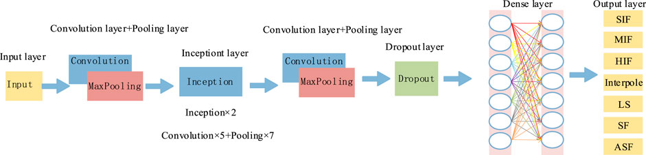
FIGURE 1. Basic model structure of CNN.

2.2.1 Forward propagation process

The convolutional neural network processes the output of the previous layer as the input of the next layer and constructs multiple filters capable of extracting input features. It can achieve the extraction of multi-sensitive features of hidden data. The essence is a mapping relationship between the input and output. The mathematical model is expressed as follows:

$x_j^l=f\left({\displaystyle \sum _{i\in M_j}}{x}_i^{l-1}*{\omega }_{ij}^l+b_j^l\right),(5)$

where $x_j^l$ is the output of the jth neuron of the layer $l$; $x_i^{l-1}$ is the input of the ith neuron of the layer $l-1$; $M_j$ is the input feature map; $l$ is the network of the layer $l$; $\omega$ is the weight matrix; $b_j^l$ is the bias of the jth neuron network of the layer $l$; and f is the activation function. In this paper, a non-linear function—ReLU—is used as the activation function. The expression is given as follows:

$f\left(x\right)=\max \left(0,x\right).(6)$

If the input is greater than 0, return the input value directly. If the output is less than or equal to 0, return 0. In contrast to the activation function tanh and sigmoid, ReLU can speed up the training of the model. It can reduce the difficulty in the calculation and has strong robustness. The gradient disappearance problem is solved to some extent.

The pool sampling layer extracts the local features. It can detect the same features under different locations with better spatial and structural invariance. There are two common sampling methods: maximum pooling and average pooling. This paper adopts the maximum pooling method. The mathematical model of the pool sampling layer is as follows:

$x_j^l=f\left({\beta }_j^{l}down\left(x_j^{l-1}\right)+b_j^l\right),(7)$

where $down\left(\right)$ is the pool sampling function; $\beta$ is the network bias. The features owned by the sampling and convolutional layers remain the same in number but decrease in size by a factor of n after pool sampling.

After several convolution and pooling oparations, a fully connected layer is used to connect the neuron weights. Softmax is used as the activation function to place the probability of each output in [0,1]. Different features are classified.

2.2.2 Backward propagation process

For classification problems, it is important to minimize the loss function of the model and improve the accuracy of the model as much as possible. The selection of the loss function is very important. The common loss functions are the root mean square error function, mean absolute error function, and cross-entropy cost function. In this paper, the cross-entropy function is selected as the loss function with the following expression:

$\left.E=-\frac{1}{n}{\displaystyle \sum _{k=1}^n}\left[y_k\ln t_k\right.+\left(1-y_k\right)\ln \left(1-t_k\right)\right],(8)$

where n is the total number of samples of the input data; t is the predicted value; and y is the actual value. In the backward propagation process, the gradient descent method is commonly used to continuously update the iterative process. The first derivative of Eq. 8 is obtained so that the network parameters can be adjusted specifically as follows:

${\omega }^{\prime }=\omega -\eta \frac{\partial E}{\partial \omega },b^{\prime }=b-\eta \frac{\partial E}{\partial b},(9)$

where ${\omega }^{\prime }$ is the updated weight; $b^{\prime }$ is the updated bias; $\omega$ is the weight before update; $b$ is the bias before update; and $\eta$ is the learning rate parameter to control the step size of the weight update.

2.2.3 Inception module

The increase in network depth or width leads to two problems in the convolutional network: 1) network parameters will increase with the increase in the number of network layers, which inevitably leads to the overfitting problem; 2) with the increase in training parameters, the training speed of the model will decrease, which makes the application of the convolution model challenging in practical engineering.

The inception module is introduced into the convolutional network. The core idea of this module is to combine different convolutional layers by parallel connection, as shown in Figure 2. Inception V1 extensively uses the convolution kernel of $5\times 5$ and $3\times 3$ and introduces the convolution kernels of $1\times 1$. It can increase the depth and width of the network, reduce the data dimension, transform the fully connected structure into sparse connections, effectively reduce the number of parameters, and significantly improve the accuracy of the model.

FIGURE 2

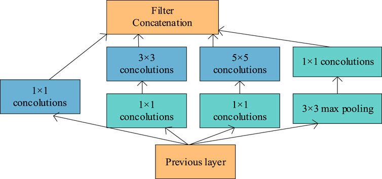
FIGURE 2. Diagram of the inception model.

2.2.4 Fault identification process

The flow of CNN-based distribution network fault identification is shown in Figure 3.

FIGURE 3

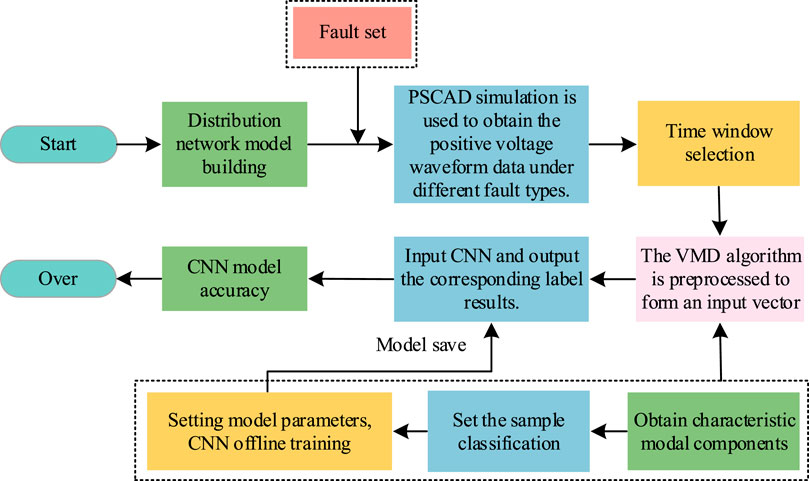
FIGURE 3. CNN fault identification process.

The steps for fault identification are as follows:

(1) Distribution network simulation data acquisition

Training of CNN models requires a large number of fault samples. In real life, two ways are commonly used to obtain the required data: 1) obtaining the recorded wave data of the actual distribution network according to its operation. 2) Simulating the structure of the actual distribution network and building the simulation model. Since distribution network faults do not occur often and the flexible DC distribution network is still in the demonstration stage, the actual engineering recorded wave data are relatively small. The first way is more difficult to obtain data to meet the required sample size. It is also more difficult to provide comprehensive coverage of various faults due to the different probabilities of occurrence of different faults. The second way can simulate the corresponding operating conditions as needed, which is a strong complement to the first way. The relevant literature proves its reliability and accuracy (de Toledo Silva et al., 2020; Krishna, 2022). The simulation test enables comprehensive multiple simulations for different faults and solves the problem of sample imbalance. PSCAD is a widely used electromagnetic transient simulation software application and has been used in a large number of simulation studies for running simulations in many types of power systems. Therefore, this paper takes the approach of obtaining the required fault waveforms by performing PSCAD simulations on the scenarios.

(2) Sample set classification

CNN training requires a large amount of data. The training samples are generally divided into the training set and test set by means of stratified sampling. All the input data are classified according to the unified division standard. The ratio of the training set to test set is generally 1:4–1:2, and the ratio used in this paper is 3:7.

(3) Time window selection

The power electronic device has limited ability to withstand inrush current. The system converter blocking time is generally 2∼5 ms. The fault time in this paper is set to 1 ms before and after the fault point, and the size of the time window is 2 ms. The fault is set to occur at 2 s, and the system sampling frequency is 20 kHz.

(4) Pre-processing of the sample set

To speed up the model solution and enable the model to converge, the eigenmodal components decomposed by VMD need to be normalized. In this paper, we use min–max normalization to map the input data into [0,1].

$x_{norm}=\frac{x-\mathit{Min}}{\mathit{Max}-\mathit{Min}}.(10)$

Define different fault labels for seven different fault types. Set different fault labels $\left[l_1,l_2,l_3,l_4,l_5,l_6,l_7\right]$ for the output of this network. The specific label classification is shown in Supplementary Exhibit S1.

(5)Building and training of the CNN model

Before training the model, the weights and biases of the convolutional kernel need to be set, with the initial value set to 0. Using the feedback from the training set results, parameters such as the number of layers, training times, and learning rate of the network are adjusted. The 1D convolutional neural network structure in this paper includes one input layer, five convolutional layers, seven pooling layers, two inception layers, two dense layers, and one output layer. The step size of convolution is set to 2, the number of training times is 300, the size of the convolutional kernel is 4, and the learning rate is 0.02. Dropout is set to 0.2. The basic idea is to let each layer of neurons randomly discard part of the training, so that these discarded parts are not activated. The next network is used as the target of this update. With each iteration, the sub-networks are updated continuously. The probability of repeated training is greatly reduced, making the model more robust.

The optimizer can calculate the gradient of the loss function in each iteration and update the parameters so that the loss function is minimized. In this paper, the adaptive moment estimation (Adam) optimization function is used, which is suitable for non-smooth objectives and has an intuitive interpretation.

(6)Construction of the confusion matrix and evaluation index

The confusion matrix is a visualization tool in deep networks to compare the predicted data with the real results. The matrix can visually characterize the accuracy of the model. Each column of this matrix characterizes the predicted category of different faults. Each row characterizes the actual fault category represented by the data, as shown in Figure 4.

FIGURE 4

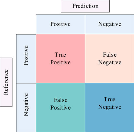
FIGURE 4. Diagram of the confusion matrix structure.

In this structure, true positive (TP) indicates that the actual value is positive and the predicted value is also positive, and true negative (TN) indicates that the actual value is negative and the predicted value is also negative. In these cases, the identification is correct. Wrong Positive (WP) indicates that the actual value is negative, but the model prediction is considered positive. False negative (FN) indicates that the actual value is positive, but the model identification is considered negative. In these cases, the identification is incorrect.

The total number of samples of the model = TP + FP + TN + FN, and the correctness (accuracy), precision (precision), recall (Recall), and F1 score of the CNN model recognition results are expressed as follows:

$\begin{array}{l}\text{Accuracy}=\frac{TP+TN}{TP+TN+FP+FN},\text{Precision}=\frac{TP}{TP+FP},\\ \text{Recall}=\frac{TP}{TP+FN},\mathrm{F}1\text{Score}=\frac{2\mathit{PR}}{P+R},\end{array}(11)$

where p denotes precision and R denotes recall.

Accuracy can represent the proportion of the predicted value of all the correct results in the classification model. Precision represents the proportion of correct values in the results where the model prediction is positive. Recall represents the proportion of correct values that the actual value is positive. The F1 score metric combines precision and recall outputs and ranges from 0 to 1. The F1 score index comprehensively considers the result of accuracy and recall rate output, ranging from 0 to 1. The closer the F1 score index is to 1, the better the model output.

3 Model building

The PSCAD/EMTDC simulation platform is used to build the ±10 kV DC distribution network structure (Figure 5). The AC-side voltage is 10 kV. The AC-side transformer adopts the Δ/Yn type via large resistance grounding. The system frequency is 50 Hz. The bridge arm reactance is 10 mH. The sub-module capacitance is 4500 uF. The number of sub-modules is 50. The cable is connected to the AC grid through a multilevel converter (MMC).

FIGURE 5

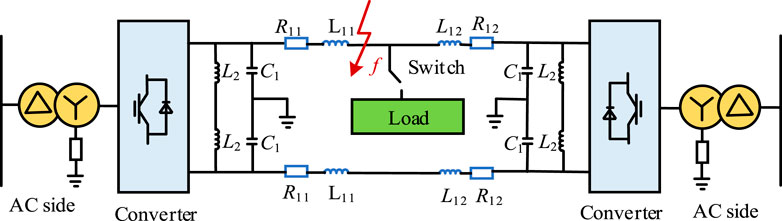
FIGURE 5. Structure of the 10-kV flexible DC distribution network.

The system is a small-current grounding system. When a single-pole ground fault occurs in a DC line, the fault current has no ground circuit. The DC line current is still rated. The system zero potential shift occurs. The grounding pole line voltage drops to 0. Non-grounding pole line voltage rises to twice the original voltage. Inter-pole voltage remains unchanged. The system can still run for 2 hours after a single-pole ground fault.

Compared to the single-pole ground fault, the inter-pole short-circuit fault in the DC distribution network is more serious. This fault will cause the current to rise sharply, and the positive and negative voltage of the ground pole will drop to 0 rapidly. The inter-pole voltage will also drop to 0. After the converter is locked, if the fault cannot be removed in time, the system will remain in this state. It will cause damage to distribution network equipment and pose a threat to personal safety (Zheng et al., 2019).

The zero-sequence voltage component in the asymmetric fault of the AC side will cause the power frequency common mode fluctuation of the positive and negative voltage of the DC side (Baoguo et al., 2021). The transient characteristics are similar to those of the DC high-resistance ground fault.

The fault line selection method based on the transient component can overcome the shortcomings of low sensitivity and poor reliability in the case of an intermittent ground fault. Due to the weak transient fault characteristics, the existence of unstable fault arc, internal and external random factors, and modern signal processing technology is widely used. Signal processing technology can be used to improve the identification and extraction ability of weak features.

Since the process of positive and negative voltage change is similar, only the positive voltage of the grounding pole is used as the characteristic pre-processing quantity in this paper.

4 Result analysis

Build the system simulation as shown in Figure 1, and obtain 200 groups of data for each fault type. For a single-pole ground fault, set the fault type to SIF, MIF, and HIF. The resistance value of SIF is set between 0 and 100 Ω. The resistance value of MIF is set between 100 Ω and 1000 Ω (Wang et al., 2014). When the HIF fault occurs, the fault point will appear as arc extinguishing and re-ignition. The arc current fluctuates at high frequency, and the grounding line pole voltage also oscillates at high frequency. It cannot be simulated by simply increasing the resistance of the grounding resistor to simulate the fault situation. The Emanuel model is widely used to accurately describe the characteristics of the HIF arc (Gautam and Brahma, 2013). This paper uses the Emanuel arc model to simulate the HIF. The specific model structure is shown in Figure 6.

FIGURE 6

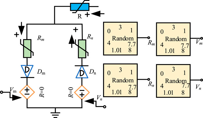
FIGURE 6. Emanuel arc model circuit diagram.

The model consists of two DC voltage sources V_m and V_n, two diodes D_m and D_n, and two variable resistors R_m and R_n. The model can simulate the characteristics of the arc under HIF. The zero rest time of the arc voltage can be adjusted by changing the value of the DC voltage. The diodes are used to reflect the different cycles of the waveform on and off. Variable resistors are used to simulate the asymmetry of the current under the fault. In this paper, the parameters are set as follows: V_m varies randomly between 0.5 and 0.8 kV, V_n varies randomly between 0.9 and 1.1 kV, R_m and R_n vary randomly between 450 Ω and 1000 Ω, and R is obtained between 800 and 3000 Ω.

For the inter-pole fault, the transition resistance is set to vary from 0 to 5 Ω. Considering that there will be a large load disturbance in the distribution network, it is necessary to take the load switching as one of the conditions. In this paper, the capacity of LS is set from 0 to 10 MW. In addition, the impact of the AC-side fault on the DC-side voltage should be considered, so two types of symmetrical and asymmetrical faults are also required on the AC side.

The seven operating conditions of the ground positive voltage fault waveforms under the selected time window are shown in Figure 7, where the fault occurs at the 0 ms moment.

FIGURE 7

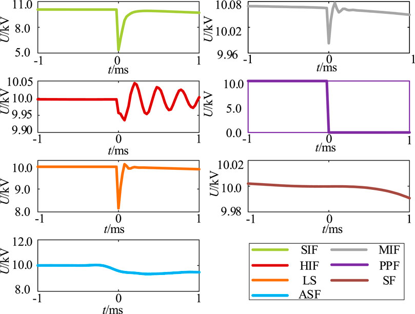
FIGURE 7. Positive voltage waveform of the grounding line under different fault conditions.

The line positive voltage drops to 5.63 kV and then slowly decreases when SIF occurs, as shown in Figure 7A. The line positive voltage fluctuates, the high-frequency component appears in the waveform, and then the voltage value slowly decreases when MIF occurs, as shown in Figure 7B. The sudden change is not so drastic when HIF occurs compared with SIF and MIF, as shown in Figure 7C. The line positive voltage under the fault has a more obvious oscillation characteristic, and the fluctuation is small and random. The line positive voltage drops to 0 kV instantaneously, and thereafter it is consistently maintained at 0 kV when PPF occurs, as shown in Figure 7D. The power transfer between converters stops. The voltage value undergoes an abrupt change when LS disturbance occurs, as shown in Figure 7E. Thereafter, it shows a steady-state response state. The voltage and current on the AC side of the converter will have a negative sequence component when the AC asymmetric fault occurs, as shown in Figure 7G, which will cause an even number of non-characteristic harmonics on the DC side, resulting in fluctuations in the voltage at the ground terminal. The simulation results remain consistent with the theoretical analysis.

4.1 VMD algorithm decomposition

To further differentiate the fault categories, VMD is used to decompose the grounding pole positive voltage to obtain the eigenmodal components IMFs. Figure 8 and Figure 9 show the IMF1 and IMF2 waveforms after VMD, respectively.

FIGURE 8

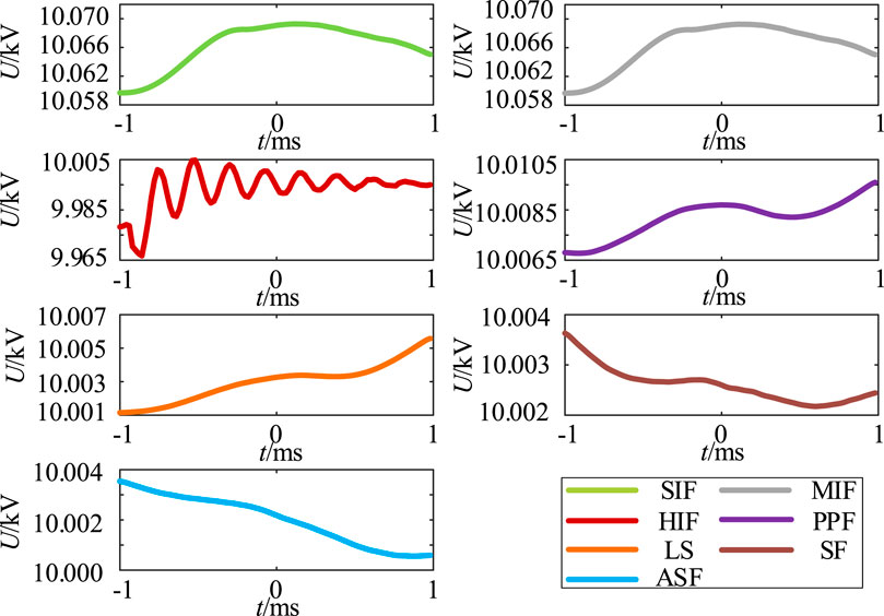
FIGURE 8. IMF1 after VMD.

FIGURE 9

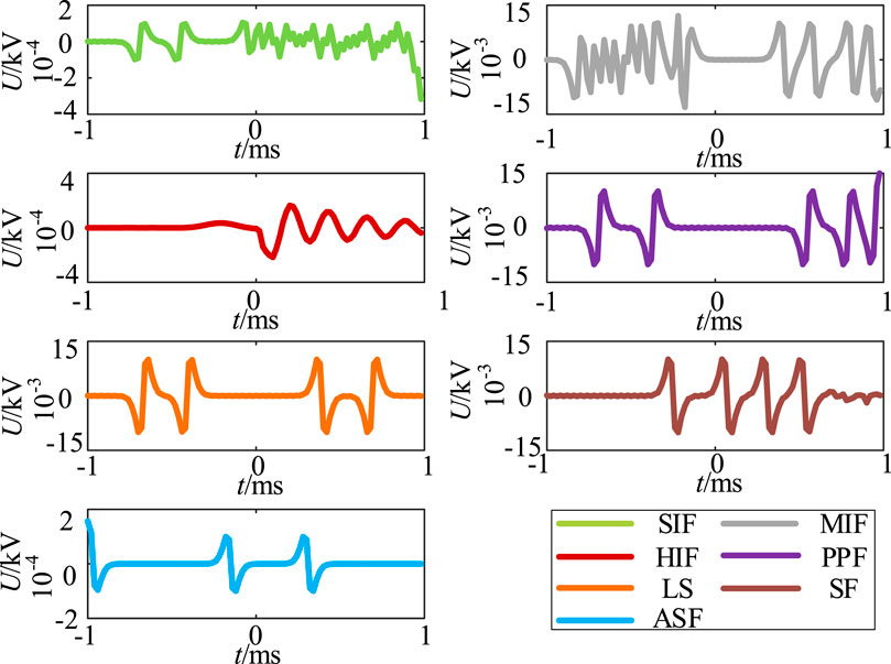
FIGURE 9. IMF2 after VMD.

As shown in Figure 8, the similarity of waveforms under different working conditions is high, such as SIF and MIF, PPF, and LS. Furthermore, there is a possibility of confusion in the subsequent model training. The decomposed results are fed into the CNN training model, and the accuracy is 90.48%. The recognition accuracy is not high, so it is not suitable to use IMF1 as the input of the training model.

As shown in Figure 9, the difference between the fault waveform and amplitude under IMF2 is high. These differences are suitable for constructing detection criteria, so IMF2 is chosen as the input data for the CNN in this paper.

4.2 CNN model training results

In order to further clarify the effectiveness and superiority of the proposed algorithm, the t-SNE method is used for visualization. The original data, the characteristic modal component IMF2 after VMD, and the CNN model training results are visualized by t-SNE. The experimental results are shown in Figure 10. Categories 0, 1, 2, 3, 4, 5, and 6 represent SIF, MIF, HIF, PPF, LS, SF, and ASF, respectively. Figure 10A shows the distribution of the original data. Due to the redundancy of the original data, various categories are difficult to distinguish and easy to confuse. Figure 10B shows the dimensionality reduction result of the characteristic modal component IMF2 after VMD, which is further distinguished from the original data. However, there is still a large overlap between categories 2, 4, and 5. Figure 10C shows the visualization of classification results after CNN model training. It can be seen that each category is clearly distinguished, which verifies that the proposed algorithm has a high fault recognition rate.

FIGURE 10

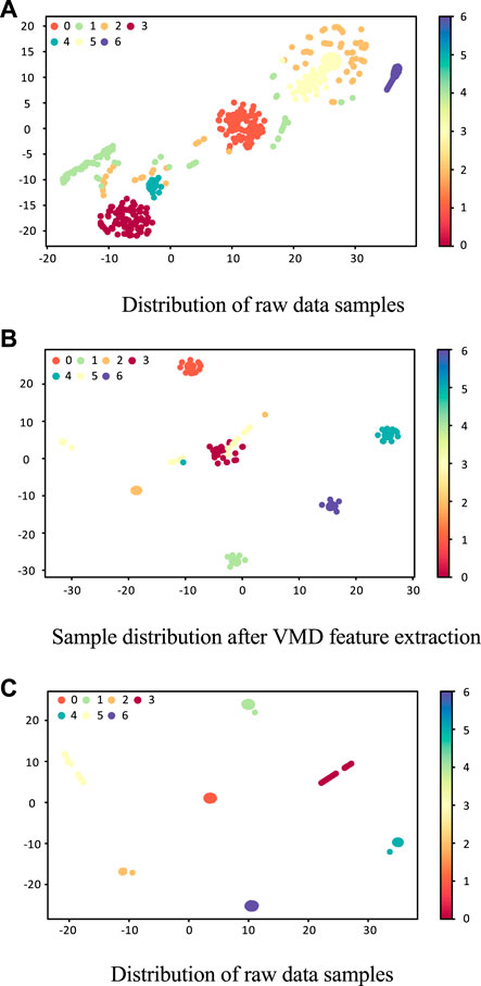
FIGURE 10. Visualization of feature learning at different stages. (A) Distribution of raw data samples. (B) Sample distribution after VMD feature extraction. (C) Distribution of raw data samples.

The pre-processed data are fed into the network. The parameters of the CNN are adjusted using the network error loss values. The total sample is randomly sampled. Figure 11 shows the CNN recognition results.

FIGURE 11

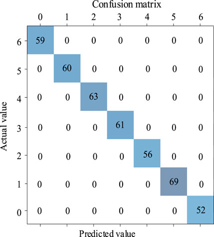
FIGURE 11. CNN recognition results.

From this confusion matrix and Supplementary Exhibit S2, the CNN trained model has 100% correctness, 100% accuracy, 100% recall, and 100% F1 score. The actual and predicted values under different faults remain the same. The probability of the detection error or omission is 0. Using the model training established in this paper, various fault types can be accurately and effectively identified.

5 Validation

5.1 Identification results after EMD

The results of using EMD to extract the characteristic modes for the seven working conditions are shown in Figure 12. The results show that although EMD can also extract the corresponding high-frequency components, the resulting modal components contain more noise components, which has some interference in the subsequent recognition accuracy.

FIGURE 12

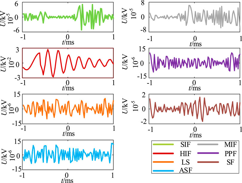
FIGURE 12. IMF2 after EMD.

The results of EMD were fed into the CNN model for training. The results are shown in Figure 13, with an accuracy of 87.62%. It is not accurate and not suitable for using the eigenmodal components decomposed by EMD as the input to the CNN model.

FIGURE 13

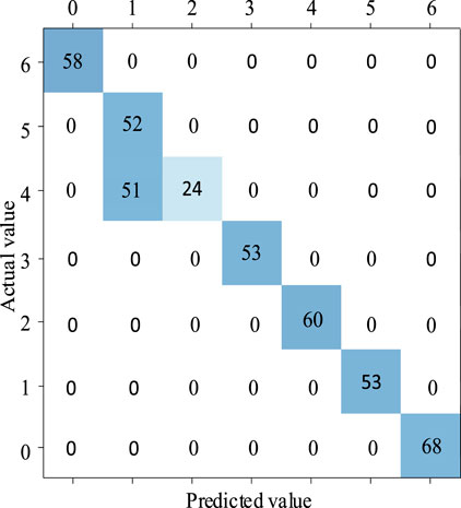
FIGURE 13. Training results of IMF2 under EMD.

5.2 Different fault locations

To test the applicability of the algorithm proposed in this paper at different faults, the situation of different faults among SIF, MIF, HIF, LS, PPF, SF, and ASF occurring at 6 km from the cable line is simulated (Figure 11 shows the training results at the fault location of 10 km). The training results at this fault location are shown in Supplementary Exhibit S3. The figure shows the training model at different fault locations. The accuracy of the training model at different fault locations is 100%. It shows that the discrimination method proposed in this paper can be applied to discriminate different fault types at different fault locations.

5.3 Adding strong noise

To verify the applicability of the algorithm proposed in this paper during strong noise, white Gauss noise with a signal-to-noise ratio of 1 db is added to the DC line pole voltage. Taking the single-pole high-resistance grounding fault as an example, the waveform of the positive voltage decomposed by VMD after adding strong noise is examined and shown in Figure 14. The addition of noise causes a certain degree of waveform fluctuation, which has some interference with the training recognition of the model.

FIGURE 14

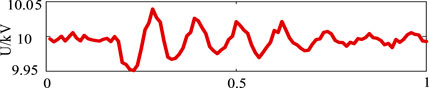
FIGURE 14. Waveform after adding noise.

The feature components after adding noise are fed into the CNN for recognition, and Figure 15 shows the recognition results with 99.76% recognition accuracy. The results show that the CNN discriminative model accuracy is still reliable under the interference of strong noise.

FIGURE 15

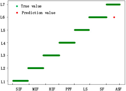
FIGURE 15. Recognition accuracy under 1 dB noise.

5.4 Change in the time window

The setting of the time window directly affects the amount of data. The more the time windows of the data, the more the test samples contained. Based on the system’s converter blocking time, the selected time window is now changed to 2 ms before and after the fault for testing. Figure 16 shows the results after VMD under the selected time window. The results are input into the CNN for training. The accuracy achieved 100%. It can be seen that the proposed discrimination method in this paper can be applied to discriminate different fault types under different time windows.

FIGURE 16

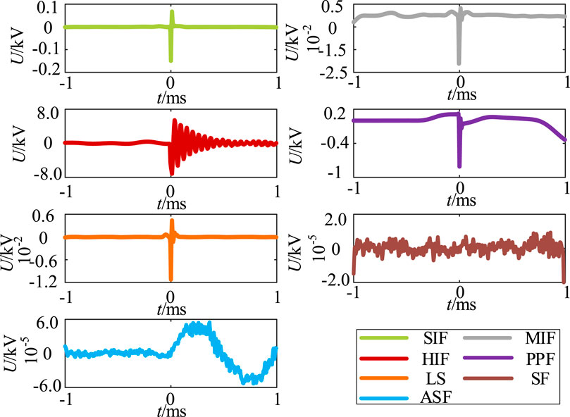
FIGURE 16. Different data window tests.

5.5 Different sampling frequencies

To verify the accuracy of the proposed algorithm, a system sampling frequency of 10 kHz is adopted. The model recognition results are shown in Figure 17. It can be seen that the proposed algorithm is still accurate and reliable under different sampling frequencies.

FIGURE 17

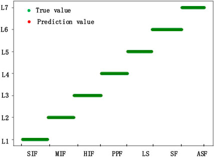
FIGURE 17. Recognition accuracy at 10 kHz sampling frequency.

5.6 Comparison with the unimproved CNN

To verify the performance of the CNN model proposed in this paper, each feature modal component decomposed by VMD is now fed into the improved inception–CNN model and the traditional CNN model. The recognition accuracy is shown in Supplementary Exhibit S4.

Supplementary Exhibit shows that the different eigenmodal components as the input of the improved CNN model proposed in this paper have significantly improved the accuracy rate compared with the traditional CNN. Overall, the accuracy rate and recall rate have also been improved. The F1 score is closer to 1 in the improved CNN model. These features indicate that the output effect of the improved inception–CNN model is more effective and is even better than the unimproved CNN performance.

6 Conclusion

In this paper, a DC distribution network fault identification scheme based on VMD and inception–CNN is proposed. It is simulated and verified in the PSCAD platform. The following conclusions can be obtained:

(1)The proposed scheme uses variational modal decomposition to process the simulation data. The processed eigenmodal components are used as the input of the training model, which has good generalization capability and anti-interference capability against noise. It also has an excellent reliability performance in different application scenarios.

(2)The proposed training model can not only identify single-pole, double-pole, and AC-side faults but also effectively discriminate the fault types with different resistance changes under single-pole faults. It has high recognition accuracy.

(3)The complex structure of the CNN model makes it possible to abstract the feature signal and effectively identify the weak changes under the high-resistance ground fault.

Data availability statement

The original contributions presented in the study are included in the article/Supplementary Material; further inquiries can be directed to the corresponding author.

Author contributions

FZ: investigation, validation, and writing–review and editing. YP: writing–original draft. CJ: supervision, visualization, and writing–review and editing. YL: conceptualization, data curation, and writing–review and editing. NL: funding acquisition and writing–review and editing. All authors contributed to the article and approved the submitted version.

Funding

The author(s) declare that financial support was received for the research, authorship, and/or publication of this article. The project was supported by the Natural Science Foundation of China (52167010).

Conflict of interest

Author YL was employed by State Grid Fujian Electric Power Company, Fuzhou Power Supply Company.

The remaining authors declare that the research was conducted in the absence of any commercial or financial relationships that could be construed as a potential conflict of interest.

Publisher’s note

All claims expressed in this article are solely those of the authors and do not necessarily represent those of their affiliated organizations, or those of the publisher, the editors, and the reviewers. Any product that may be evaluated in this article, or claim that may be made by its manufacturer, is not guaranteed or endorsed by the publisher.

Supplementary material

The Supplementary Material for this article can be found online at: https://www.frontiersin.org/articles/10.3389/fenrg.2023.1258619/full#supplementary-material

References

Bagheri, A., Gu, I. Y. H., Bollen, M. H. J., and Balouji, E. (2018). A robust transform-domain deep convolutional network for voltage dip classification. IEEE Trans. Power Deliv. 33 (6), 2794–2802. doi:10.1109/tpwrd.2018.2854677

CrossRef Full Text | Google Scholar

Baoguo, Z., Yake, J., Lei, Z., Di, S., Lei, W., and Shengbin, Y. (2021). “Effects of AC side fault on DC side fault characteristics in flexible DC distribution system,” in Proceedings of the 10th Renewable Power Generation Conference (RPG 2021), Online Conference, October 2021, 904–909. doi:10.1049/icp.2021.2360

CrossRef Full Text | Google Scholar

Chopdar, S. M., and Koshti, A. K. (2022). “Fault detection and classification in power system using artificial neural network,” in Proceedings of the 2022 2nd International Conference on Intelligent Technologies (CONIT), Hubli, India, June 2022, 1–6.

CrossRef Full Text | Google Scholar

de Toledo Silva, F. A., Komatsu, W., and Antonio Jardini, J. (2020). “Use of DC/DC converters modeled as AC-DC converters in HVDC Grids,” in Proceedings of the 2020 IEEE PES Transmission and Distribution Conference and Exhibition - Latin America (T&D LA), Montevideo, Uruguay, September 2020, 1–6. doi:10.1109/TDLA47668.2020.9326156

CrossRef Full Text | Google Scholar

Gautam, S., and Brahma, S. M. (2013). Detection of high Impedance Fault in power distribution systems using mathematical morphology. IEEE Trans. Power Syst. 28 (2), 1226–1234. doi:10.1109/TPWRS.2012.2215630

CrossRef Full Text | Google Scholar

Kiranyaz, S., Gastli, A., Ben-Brahim, L., Al-Emadi, N., and Gabbouj, M. (2019). Real-time Fault Detection and identification for MMC using 1-D convolutional neural networks. IEEE Trans. Ind. Electron 66 (11), 8760–8771. doi:10.1109/tie.2018.2833045

CrossRef Full Text | Google Scholar

Krishna, S. V. (2022). “Power quality analysis of solar plant by measurement at site and through simulation in PSCAD,” in Proceedings of the2022 Second International Conference on Power, Control and Computing Technologies (ICPC2T), Raipur, India, March 2022, 1–6. doi:10.1109/ICPC2T53885.2022.9776999

CrossRef Full Text | Google Scholar

Liu, X. (2022). “Fault detection model based on FFT-HHT analysis method,” in Proceedings of the 2022 7th International Conference on Intelligent Computing and Signal Processing (ICSP), Xi'an, China, April 2022, 972–975. doi:10.1109/ICSP54964.2022.9778785

CrossRef Full Text | Google Scholar

Naidu, S. M. (2022). “HVDC Fault detection and Identification in monopolar topology using deep learning,” in Proceedings of the2022 12th International Conference on Power, Energy and Electrical Engineering (CPEEE), Shiga, Japan, February 2022, 354–358. doi:10.1109/CPEEE54404.2022.9738716

CrossRef Full Text | Google Scholar

Robertas, D., Christian, N., Tatjana, S., and Woźniak, M. (2017). IMF mode demixing in EMD for jitter analysis. J. Comput. Sci. 22, 240–252. doi:10.1016/j.jocs.2017.04.008

CrossRef Full Text | Google Scholar

Routray, P., Mishra, M., and Rout, P. K. (2015). “High Impedance Fault detection in radial distribution system using S-Transform and neural network,” in Proceedings of the 2015 IEEE Power, Communication and Information Technology Conference (PCITC), Bhubaneswar, India, October 2015, 545–551. doi:10.1109/PCITC.2015.7438225

CrossRef Full Text | Google Scholar

Sarwagya, K., and Ranjan, S. (2020). “Detection and classification of faults in distribution system using signal processing techniques,” in Proceedings of the 2020 International Conference on Computer, Electrical and Communication Engineering (ICCECE), Kolkata, India, January 2020, 1–6. doi:10.1109/ICCECE48148.2020.9223072

CrossRef Full Text | Google Scholar

Satpathi, K., Yeap, Y. M., Ukil, A., and Geddada, N. (2018). Short-time fourier transform based transient analysis of VSC interfaced point-to-point DC system. IEEE Trans. Industrial Electron. 65 (5), 4080–4091. doi:10.1109/tie.2017.2758745

CrossRef Full Text | Google Scholar

Sharma, N. K., Samantaray, S. R., and Bhende, C. N. (2022). VMD-enabled current-based fast Fault Detection scheme for DC microgrid. IEEE Syst. J. 16 (1), 933–944. doi:10.1109/JSYST.2021.3057334

CrossRef Full Text | Google Scholar

Silva, S., Costa, P., Gouvea, M., Lacerda, A., Alves, F., and Leite, D. (2018). High impedance fault detection in power distribution systems using wavelet transform and evolving neural network. Electr. Power Syst. Res. 154, 474–483. doi:10.1016/j.epsr.2017.08.039

CrossRef Full Text | Google Scholar

Song, X., Wang, S., and Dong, X. (2022). “Research on Fault Detection scheme for hybrid LCC-MMC system,” in Proceedings of the 2022 7th Asia Conference on Power and Electrical Engineering (ACPEE), Hangzhou, China, 1309–1313.

CrossRef Full Text | Google Scholar

Song, Y., Hou, G., and Wang, S. (2021). “DC Fault Detection method for DC grids based on frequency domain voltage characteristics,” in Proceedings of the 2021 6th International Conference on Power and Renewable Energy (ICPRE), Shanghai, China, September 2021, 196–201.

CrossRef Full Text | Google Scholar

Taheri, B., and Razavi, F. (2018). Power swing detection using rms current measurements. J. Electr. Eng. Technol. 13 (5), 1831–1840. doi:10.5370/JEET.2018.13.5.1831

CrossRef Full Text | Google Scholar

Wang, X., Gao, J., and Wei, X. (2014). A fault line selection method of small current grounding system based on wavelet packet and Bayes theory. Industry Mine Automation 40 (6), 54–59. doi:10.13272/j.issn.1671-251x.2014.06.014

CrossRef Full Text | Google Scholar

Xiang, W., Yang, S., Xu, L., Zhang, J., Lin, W., and Wen, J. (2019). A transient voltage-based DC fault line protection scheme for MMC-based DC grid embedding DC breakers. IEEE Trans. Power Deliv. 34 (1), 334–345. doi:10.1109/TPWRD.2018.2874817

CrossRef Full Text | Google Scholar

Xu, H., Huang, F., and Fang, Y. (2021). “Fault signal analysis of rolling bearing based on CEEMDAN decomposition method,” in Proceedings of the 2021 International Conference on Computer Information Science and Artificial Intelligence (CISAI), Kunming, China, September 2021, 918–922. doi:10.1109/CISAI54367.2021.00184

CrossRef Full Text | Google Scholar

Yao, W., Gao, X., Wang, S., and Liu, Y. (2019). “Distribution high Impedance Fault Detection using the fault signal reconstruction method,” in Proceedings of the 2019 IEEE 3rd Conference on Energy Internet and Energy System Integration (EI2), Changsha, China, November 2019, 2573–2577. doi:10.1109/EI247390.2019.9061798

CrossRef Full Text | Google Scholar

Zheng, Q., Ni, X., Lv, F., and Huang, X. (2019). “Inter-Pole short circuit protection strategy for flexible DC distribution network converter valve and differential combination,” in Proceedings of the2019 International Conference on Artificial Intelligence and Advanced Manufacturing (AIAM), Dublin, Ireland, October 2019, 725–729. doi:10.1109/AIAM48774.2019.00150

CrossRef Full Text | Google Scholar

Zheng, Y., Mao, M., and Chang, L. (2021). “DCSCF detection method of MMC-DC-grid based on statistical feature and DBN-SOFTMAX,” in Proceedings of the 2021 IEEE 12th International Symposium on Power Electronics for Distributed Generation Systems (PEDG), Chicago, IL, USA, June 2021, 1–6.

CrossRef Full Text | Google Scholar