A revision of blade element/momentum theory for wind turbines in their high-thrust region

Abstract
Modern horizontal-axis wind turbines produce maximum power at an optimal tip speed ratio, λ_opt, of around 7. This is also the approximate start of the high-thrust region, which extends to runaway at λ_R ≈ 2λ_opt where no power is produced and the thrust is maximized. The runaway thrust coefficient often exceeds unity. It is well known that the conventional axial momentum equation must be modified whenever the thrust coefficient approaches unity, but most past modifications have no sound physical basis. Our main revision is to include the “wake vorticity” term in the axial momentum balance. This term is related to blade element drag and acts to decouple the thrust from the induced axial velocity when it becomes large near the edge of the rotor as the runaway is approached. The wake vorticity term dominates the axial momentum equation in these conditions and leads to estimates of power and thrust that are consistent with the limited amount of high-quality experimental data in the high-thrust region.

1 Introduction

The blade element theory (BET) divides the blades of a horizontal-axis wind turbine into a contiguous stack of radial elements, typically 30–50 in number. They are assumed to behave as airfoils whose lift and drag give the element’s thrust and torque. These are balanced against the axial and angular momentum changes in the annular streamtube flowing over the element derived from momentum theory (MT). The combined blade element/momentum theory (BEMT) is the workhorse of wind turbine aerodynamics. BEMT is described in all aerodynamics text books and is widely used in the initial, multidimensional design of blades, for which the potentially more accurate computational fluid dynamics modeling is prohibitively costly in computer time, e.g., Sessarego et al. (2015).

Wind turbine performance is usually considered in terms of the power and thrust coefficients, C_P and C_T, respectively, as functions of the tip speed ratio, λ = ΩR/U₀, where Ω is the blade angular velocity, R is the tip radius, and U₀ is the wind speed. BEMT is generally held to provide accurate estimates of C_P and C_T in comparison to wind tunnel and field tests, as shown in Spera (1994), Wood (2011), and Schmitz (2020). It is well known, however, that the relation between the induced axial velocity at the rotor, u, and in the far-wake, u_∞, u = (1 + u_∞)/2 in the one-dimensional version of the momentum theory starts to break down somewhere near the tip speed ratio for maximum power, λ_opt. This is the start of the high-thrust region: as λ increases further, C_T approaches and sometimes exceeds unity, the maximum value allowed by conventional momentum theory. The high-thrust region for wind turbines ends at the runaway tip speed ratio, λ_R, where C_P = 0 and C_T = C_TR is usually maximized if λ_R is large (Note that the subscript “R” denotes runaway values, whereas the script “R” is the rotor radius). Since modern turbines have λ_opt ∼ 7 − 9, the high-thrust region normally spans high values of λ: as a rule of thumb λ_R ≈ 2λ_opt. This approximate relation holds for multiblade windmills where λ_opt ∼ 1, as shown in Figure 5 of John et al. (2023), and the experiments of Krogstad and Adaramola (2012) and Krogstad and Eriksen (2013) that we consider below, for which λ_opt ∼ 6. Furthermore, it is normal for C_T to increase monotonically in this region when λ_opt is large.

Pratumnopharat and Leung (2011) and Schmitz (2020) documented a large number of modifications that have been made to the relationship between C_T and u for the high-thrust region. It is our contention that these modifications are ad hoc, have little or no physical basis, and rely on questionable experimental results obtained a century ago, as explained in Section 2.7 of Wood (2011). Unfortunately, there have been very few subsequent experiments on the high-thrust region that provide sufficient detail for BEMT revision. One of the few that does was by Limacher et al. (2022), who measured the thrust and all three velocities in the wake of a small model turbine by particle image velocimetry, for values of λ above and below λ_R = 7.9. They proposed a revision to the conventional momentum equation that will be described later. The other measurements in this category were by Krogstad and Adaramola (2012) and Krogstad and Eriksen (2013), who provided power, thrust, and limited wake measurements for a model wind turbine with λ_opt ≈ 6 and λ_R ≈ 12. Their results will be compared to the revised BEMT developed here.

Our further contention is that BET remains valid in the high-thrust region, but the conventional angular and axial momentum equations are incomplete. The most important omission is in the latter equation, which should contain a term related to the “wake vorticity.” This term balances the BE drag on stationary turbines but increasingly balances the BE lift (and thrust) as λ increases. It also decouples the approach to the runaway from the relationship between u and u_∞. Our revised BEMT equations require no specific relation between the two velocities.

The wake vorticity term was identified in the computational study of the flow through two-dimensional, equi-spaced cascades of airfoils by Golmirzaee and Wood (2023). Cascade elements are subjected to the same forces as wind turbine blade elements and have the same MT terms except for those due to expansion, rotation, and the vorticity shed from the blades as a consequence of the radial gradient of the bound vorticity. The wake vorticity term is introduced in the following section after the following preliminary observations on the induced velocities u and w in the circumferential direction. One of the key simplifications of MT is that the wake is characterized by circumferential averages of u and w. When the number of blades, N, is finite and λ is small, the velocities at the elements, which determine the lift and drag, may differ from their streamtube averages. This difference is usually accommodated by the use of “finite blade functions:” F_u = u/u_b and F_w = w/w_b, where the subscript “b” denotes a value at the blades. Nearly all BEMT codes for wind turbines use Prandtl’s tip loss factor, F_P to approximate F_u and F_w. Some of the inaccuracies of using F_P are documented in Wood et al. (2016) and Wood (2021), while Wood et al. (2021) reviewed the numerical methods that produce accurate estimates for F_u and F_w. Wood et al. (2016) showed that F_u, F_w → F_p and F_p → 1 as λ increases, suggesting that azimuthal variations become less important in the high-thrust region.

Our revisions to BEMT apply at all values of λ including zero, but we concentrate on the high-thrust region, where BEMT is most challenged. It is further noted that John et al. (2023) found conventional BEMT accurately predicted λ_R for a model of a low-speed, multi-bladed water pumping windmill where λ_R ≈ 2 and the runaway C_TR increased from 0.1 to 0.5 as N increased from 3 to 24. The implication is that the present revisions are not critical at low λ.

Our major aim is to establish the necessity to include the wake vorticity term in the axial momentum equation. This may not be the only change to MT necessary for accurate calculation of the high-thrust region, but we show that it is likely to be a very important one. We argue that more experimental information near the runaway is required to complete the revision of BEMT.

The rest of this paper is laid out as follows. Section 2 describes BEMT and our revision. We use a simple version of the revision in Section 3 to compute the power and thrust as the runaway is approached and compare these to wind tunnel measurements by Krogstad and Adaramola (2012) and Krogstad and Eriksen (2013) on a model three-bladed rotor. Section 4 focuses on further requirements for completing the revision of BEMT and the conclusions.

2 Blade element/momentum theory

Using the definitions of the velocity at the blade element, U_rel, and the angle ϕ from Figure 1, the balance between the gradient of thrust, dT/dr, and the axial momentum flux for an N − bladed rotor at radius r is given as follows:

$\frac{dT}{dr}=\frac{1}{2}N\rho U_{rel}^{2}c\left(C_l\cos \varphi +C_d\sin \varphi \right)=\pi \rho \left(4\overline{w^2}+4\lambda rw+\overline{v^2}-\overline{u^2}\right)r,(1)$

where ρ is the density of air and c is the blade element chord. C_l and C_d are the lift and drag coefficients, respectively. They are functions of the angle of attack, α, which—according to Figure 1—is dependent on u_b and w_b. The term on the right involving u, w, and the radial velocity v is the axial momentum flux in the annular streamtube intersecting the N elements. It is important to note that w is the value at the blades, whereas the value immediately behind them is 2w. An overbar denotes a circumferential average over the streamtube for a quadratic quantity: overbars are not used on u or w on their own as their circumferential variation is important only in distinguishing values at the blades, which are subscripted as defined previously. u and w denote streamtube averages throughout this study. The last term, involving $\overline{v^2}-\overline{u^2}$, is called the “expansion” term because

${\int }_0^{\infty }\left(\overline{v^2}-\overline{u^2}\right)rdr=0,(2)$

which shows the expansion term re-distributes, rather than generates, T. Wood and Limacher (2021) showed that the expansion term gives the thrust due to the pressure acting on the expanding streamtubes upwind of the rotor. Eq. 2 ensures that v and u have the same magnitude at the rotor plane. Thus, significant flow expansion must occur when u is large.

FIGURE 1

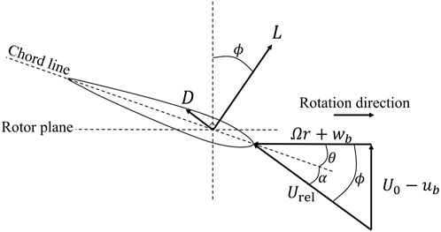
FIGURE 1. Blade element at radius r, the forces, and velocities. The wind direction is up. L is the element lift which is normal to U_rel, and D is the drag, parallel to U_rel. Ω is the angular velocity of the blades and θ is the pitch angle. The other symbols are defined in the text.

The usual thrust equation from MT ignores the expansion term and contains terms in u instead of w on the right side of Eq. 1, which is the Kutta–Joukowsky form of the momentum flux. It, along with Eq. 2, was derived by Limacher and Wood (2021) using a control volume (CV) of radius much larger than R, with the inlet far upwind of the rotor where u = v = w = 0, and the outlet immediately behind the blades. Eqs 1, 2 hold for any amount of wake expansion at any λ. Their relation to the usual thrust equation is easily derived by ignoring circumferential variations and the expansion term. Wood and Hammam (2022) showed that the high−λ circumferentially uniform wakes of optimal rotors satisfy “helical symmetry:” pu = wr where p = (1 − u)/(w/r + λ) is the pitch of the helical vorticity. Applying these equations turns the right side of Eq. 1 (when $\overline{v^2}-\overline{u^2}$ is ignored) into the usual form involving u:

$4\pi w\left(w+\lambda r\right)r\to 4\pi u\left(1-u\right)r,(3)$

which leads to a less general axial momentum equation than Eq. 1.

The equation for the torque, Q, derived from the same CV has the similar and familiar form:

$\frac{dQ}{dr}=\frac{1}{2}N\rho U_{rel}^{2}c\left(C_l\sin \varphi -C_d\cos \varphi \right)r=4\pi \rho \left(w-\overline{uw}\right)r^2.(4)$

For steady operation, the power extracted from the wind is the product of the rotor torque, obtained by summing Eq. 4 over all elements, and Ω: in the non-dimensional form, C_P = λC_Q, where C_Q is the standard torque coefficient.

We will assume that the BE parts of Eqs 1, 4 involving the lift and drag do not need revision. The validity of this “airfoil assumption” is difficult to assess. Simulations of the 2D cascade flow suggest it is conservative, because the lift:drag ratio for a cascade element is slightly greater than that on the corresponding airfoil, Golmirzaee and Wood (2023), but we know of no other direct assessment of the assumption for wind turbines.

We now revise the right side of Eqs 1, 4 based on the cascade simulations of Golmirzaee and Wood (2023). The revision is different from that of Limacher et al. (2022), who simplified the equations by assuming the shed vorticity was strain-free. They did not make a direct connection to blade element drag, and no consideration was given to the angular momentum equation. Their model and its relation to the current revision are considered in the following sections. For an infinite cascade of identical and equi-spaced airfoils, the BE or left sides of Eqs 1, 4 are unchanged except for the removal of N. For a cascade element, Golmirzaee and Wood (2023) show that Eq. 1 becomes

$\frac{1}{2}{U}_{rel}^{2}c\left(C_l\cos \varphi +C_d\sin \varphi \right)=2S\overline{w^2}+{\int }_{-S/2}^{S/2}\left(1-u\right){\mathrm{\Omega }}_{z}ydy,(5)$

when the density is removed. The cascade element spacing, S, is related to the circumferential distance between blade elements by S = 2πr/N, and there is no term corresponding to λrw in Eq. 1 as the cascade is stationary. Ω_z is the (transverse) vorticity, distinguished from the angular velocity by its subscript, and y is the normal co-ordinate, whose origin is the blade quarter-chord. The integral, which we call the “wake vorticity” integral or term, has no counterpart in the current form of the BEMT equation.

Eqs 1.5 and 1.6 of Liu et al. (2015) and Eq. (9.1.20) of Wu et al. (2015) give important constraints on wake vorticity:

$\underset{-S/2}{\overset{S/2}{\int }}{\mathrm{\Omega }}_z\mathrm{d}y=0\text{and}\underset{-S/2}{\overset{S/2}{\int }}\left(1-u\right){\mathrm{\Omega }}_z\mathrm{d}y=0.(6)$

The former, which relies on the applicability of the slender flow approximation Ω_z ≈ − ∂u/∂y, prevents Ω_z from contributing to the bound vorticity of the blade because it forces the area integral of Ω_z over the wake to be zero. The latter is exact for any wake independent of the validity of the slender flow approximation. It has two important consequences. First, the choice of origin for y has no effect on the wake vorticity integral. Second, it removes the integral containing Ω_z from the y−direction force balance and, by implication, from the angular momentum equation for BEMT because the integrand is (1 − u)Ω_zx. From here on, the phrase “wake vorticity term” will be used only for the integral in Eq. 5 or the corresponding integral in the axial momentum equation for BEMT. The exact y−direction cascade equivalent of Eq. 4 without the density is as follows:

$\frac{1}{2}{U}_{rel}^{2}c\left(C_l\sin \varphi -C_d\cos \varphi \right)=2S\left(w-\overline{uw}\right),(7)$

showing that the cascade analysis retains the non-linear terms from Eqs 1, 4. Golmirzaee and Wood (2023) found that the spatial variations in the velocities caused only small differences between $\overline{uw}$ and uw or between $\overline{w^2}$ and w². It is reasonable, then, to assume that significant circumferential variations in u and w for BEMT arise only through the shed vorticity, as explained previously for F_u and F_w. Furthermore, if F_u and F_w are close to unity, then it is reasonable to also ignore any circumferential variation in u², w², and uw in the high-thrust region.

For wind turbines, the wake vorticity is largely radial and is associated with the element drag. The shed vorticity arises from radial gradients in the bound circulation and lies predominantly in the radial direction. The wake expansion will cause the shed vorticity to have a radial component, so the main difference between wake and shed vorticity is that the latter can follow the local streamlines and so be force-free, whereas the former cannot. A further distinction is that an ideal rotor has shed but no wake vorticity, whereas a real rotor can have a wake without shed vorticity in the unlikely event of constant bound circulation along the blades.

2.1 Revision of the axial momentum equation

Aside from comparing Eqs 1–5, the incompleteness of the right or MT side of Eq. 1 can be shown by the following thought experiment involving a symmetrical airfoil, such as NACA 0012, at zero incidence. This airfoil is also a stationary, two-bladed wind turbine (with no center body and infinite R), and so BEMT applies. As the airfoil has no lift, w = 0 in Eq. 1 and the drag (at ϕ = π/2) is not balanced. Golmirzaee and Wood (2023) found that the wake vorticity term in Eq. 5 balanced the element drag for the corresponding situation in a cascade. Liu et al. (2015) showed the same balance for airfoils in their Eq. 1.8.

Golmirzaee and Wood (2023) reduced the wake vorticity term to the usual integral involving u for the drag, D, on anybody in an unbounded two-dimensional flow:

$D=\rho U_0^2{\int }_{-\infty }^{\infty }u\left(1-u\right)dy,(8)$

but this derivation requires the validity of the slender-flow approximation at the outlet of the CV. As λ increases, however, the approximation eventually ceases to hold anywhere in the wake, and the wake vorticity term cannot be rewritten in a form that involves only u and w. Its magnitude also increases as the angle between the wake and the plane of rotation decreases and ϕ → 0 in Figure 1. Small ϕ means the wake crosses most of the outlet of the CV used to derive the MT equations rather than being a thin wake leaving the CV near-normally as for airfoils or rotors and cascades with high ϕ. This is demonstrated in Figures 2, 3 for cascade Case 4 in Table XI of Golmirzaee and Wood (2023), for which θ = 0 and ϕ = α ≈ 4°: the wake leaves the CV at an acute angle at low ϕ, there is no region of uniform u, and the flow is filled with wake vorticity. The first constraint of Eq. 6 is approximately satisfied, and the second is satisfied within numerical uncertainty. Furthermore, the wake vorticity integrand is positive over most of the wake and cannot be simplified by the slender flow assumption as Ω_z has extrema close to where ∂U/∂y = 0. Nevertheless, Eq. 18 of Golmirzaee and Wood (2023)

$\rho {\int }_{-S/2}^{S/2}\left(1-u\right){\mathrm{\Omega }}_{z}ydy=\frac{\rho U_{rel}^{2}c{C}_d}{2\sin \varphi }.(9)$

was found to be accurate for cascade geometries that mimic the blade element flow for a wide range of λ. It may be objected that the wake vorticity integral in Eq. 9 should be reducible to an equation like Eq. 8 at least for large ϕ. This appears impossible because of a subtle difference between u in that equation and Eq. 9, and u in Eq. 3. In Eq. 8, u is the y−dependent departure from U₀ normalized by U₀ for a non-expanding flow, whereas u in the BEMT equations is the average induced velocity at the rotor. This u clearly does not have a circumferential variation.

FIGURE 2

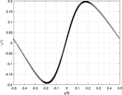
FIGURE 2. Profile of the induced axial velocity 1.29c downstream of a cascade of NACA 0012 airfoils with θ = 0, α ≈ 4°, and the spacing-to-chord ratio, S/c = 5 [case 4 in Table XI of Golmirzaee and Wood (2023)]. The origin for y is the airfoil quarter-chord.

FIGURE 3

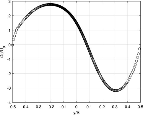
FIGURE 3. Simulation of the wake vorticity for the conditions in Figure 2.

The corresponding term for BEMT is most conveniently subtracted from the right side of Eq. 1 to give the revised form as follows:

$\begin{array}{cc}\hfill \frac{d{T}_{*}}{dr}& =\frac{1}{2}N\rho U_{rel}^{2}c\left(C_l\cos \varphi +C_d\sin \varphi -C_d/\sin \varphi \right)\hfill \\ \hfill & =\pi \rho \left(4\overline{w^2}+4\lambda rw+\overline{v^2}-\overline{u^2}\right)r,\hfill \end{array}(10)$

where T* will be called the “reduced thrust.” The right side gives the “ideal” element momentum flux—the total flux when C_d = 0. When ϕ = π/2 at λ = 0 and C_l = 0, the reduced thrust and the ideal momentum flux are both zero, which is not the case for (1). As λ increases and ϕ decreases, the wake vorticity term balances increasing amounts of lift for a wind turbine and lessens the burden on w, or u if the conventional equation was revised.

If any revisions of Eq. 4 are much less significant than the difference between Eq. 1 and Eq. 10, a number of important results follow. Eq. 4 gives the first condition for runaway as follows:

• w_R = 0 and Eq. 4 and Eq. 10 both require

• tan ϕ_R = C_d/C_l ≈ (1 − u_bR)/(λ_Rr). It then follows from Eq. 10 that

• runaway thrust is balanced entirely by the wake vorticity term.

Now, helical symmetry requires either u = 0 or p = 0 when w = 0. We regard u = 0 as physically untenable, so additional conditions are

• p_R ≈ 0 and

• u_R ≈ 1.

These five conditions can only be approximated as the wake vorticity term becomes infinite as ϕ, p_R → 0 and u_R → 1. It is also possible that w changes sign across the wake to give zero rotor torque without every element torque being zero. It will be shown below that high u was measured behind a model turbine approaching the runaway. High u implies high u_b since U₀ ≥ u_b ≥ u. Thus, it is reasonable to assume that F_u, F_w, F_p → 1 as λ → λ_R even faster than they do normally as λ increases. The simulations of the high-thrust region in the following section use F_u = F_w = 1 ∀ r. The spatial variations in the non-linear terms $\overline{u^2}$, $\overline{w^2}$, and $\overline{uw}$ in the MT equations will also be ignored, and it will be assumed that $\overline{u^2}=u^2$, $\overline{w^2}=w^2$, and $\overline{uw}=uw$. By ignoring any difference between u and u_b and assuming u is constant with r, it is possible to estimate its value from the conditions mentioned. Two additional assumptions are needed: c ∼ 1/r for optimal blades, e. g., Wood (2011) Eq. 5.12a, and C_d ≈ C_d0, the drag coefficient when α = 0, for all elements. In other words, the same or very similar airfoil(s) is/are used for the whole blade, which is usually the case for small wind turbines and wind tunnel models such as that used by Krogstad and Adaramola (2012) and Krogstad and Eriksen (2013). It then follows that

$C_{TR}\approx \frac{N{\lambda }_R^{3}c\left(R\right)c_{d0}}{3\pi \left(1-u_R\right)}.(11)$

For the three-bladed rotor of Krogstad and Adaramola (2012) and Krogstad and Eriksen (2013), C_l0 ≈ 0.5, C_d0 ≈ 0.01, and c(R) = 0.06. They found λ_R ≈ 12 and C_TR ≈ 1.2. Eq. 11 then gives u_R = 0.725, and it follows that p_R = 0.02R so the blade wake and the shed vorticity exit the CV at very small angles to the plane of rotation, as argued previously. The wake measurements closest to the runaway were made at λ = 10 at distance R behind the blades. u was approximately linear in r reaching u = 0.81 at r = 0.91. This extraordinary result has received little attention.

The importance of the wake vorticity term in the high-thrust region is now clear. Furthermore, it increases at least as fast as λ³, whereas the first and second terms on the left side of Eq. 10 vary at most as λ² and λ, respectively. It is likely, therefore, that wake vorticity will be an important term in a fully revised BEMT for any rotor at high λ. Wake vorticity also requires λ_R → ∞ as C_d ↓ 0. In other words, an ideal rotor (without drag) does not have a high-thrust region. The classical one-dimensional analysis that leads to the Betz–Joukowsky limit ignores drag and so gives no hint of a runaway. Using an actuator disc model of an ideal rotor, Wood and Hammam (2022) found that the Betz–Joukowsky values of C_P = 16/27 and C_T = 8/9 were approached as λ → ∞: ideal rotors do not run away. Thus, blade element drag is sufficient to cause a high-thrust region but it may not be the only mechanism to cause a runaway. For example, the shed vorticity modification of Limacher et al. (2022) also provides good estimates of C_T in the high-thrust region.

In considering the high-thrust region, the main difference between the blade and cascade elements is that the wakes of the former can also contain shed vorticity from the radial variation in the blade loading. Thus, it is not possible to distinguish between the MT revision due to Limacher et al. (2022) and the present revision on the basis of cascade analysis. One further comment is in the order: the present revision of MT makes no assumptions about the flow downwind of the rotor. This is a crucial point because eventually the wake vorticity will be rolled up with the shed vorticity and the distinction between them will be lost. We discuss wake development further in Section 4.

To conclude this section, we summarize the implementation of the simple model for the high-thrust region. After dividing the rotor into blade elements, Eq. 10 for the reduced thrust is solved for w, which gives Γ. The expansion term involving $\overline{v^2}-\overline{u^2}$ is ignored, $\overline{w^2}$ is approximated as w², and the difference between w and w_b is also ignored. In other words, F_u = F_ww = 1. Then, Eq. 4 is used to find u with $\overline{uw}=uw$ or F_uw = F_w = 1. For comparison, u was also computed using the helical symmetry relation pu = wr. Knowing u_b = u and w_b = w allows the determination of the torque and thrust on the blade elements. The BEMT equations for each element were iterated until a relative convergence tolerance of 10^–8 was achieved.

3 Results from the simple revised theory

We now test the plausibility of the revised BEMT. The experiments for comparison are those previously mentioned by Krogstad and Adaramola (2012) and Krogstad and Eriksen (2013) on a three-bladed rotor with R = 1.5 m. The airfoil (S826) lift and drag data, extracted from Bartl et al. (2019), cover the range of Reynolds number, Re, of the experiments. C_l(α, Re) and C_d(α, Re) were found by linear interpolation in α and log(Re).

The results for power and thrust using N_BE = 40 are shown in Figure 4. Table 1 lists the variation in C_P and C_T for N_BE = {20, 40, 80} for λ = 6 which is close to λ_opt, and λ = 12, near λ_R. All subsequent results were obtained with N = 40. The experimental results have not been corrected for blockage, which was about 10% (Sarlak et al., 2016). Using computational modeling of the experiment, Sarlak et al. (2016) found that C_P was under-estimated by around 0.05, and the corrected λ_R value was closer to 12 (their Fig. 13). Figure 14 of Sarlak et al. (2016) suggests that a blockage correction would reduce C_T by approximately the same amount. It appears that applying blockage corrections to the experimental data would generally improve the accuracy of the simple model but no correction has been applied. As expected for a BEMT analysis without finite blade corrections, C_P is over-estimated near λ_opt. The largest measured C_P at λ = 6.164 was 0.4481, which is about 10% lower than the value at λ = 6 shown in Table 1. C_T is generally under-estimated, but the trends of power and thrust and the estimate for λ_R ≈ 12 are encouraging. Furthermore, the simple model appears to have no problems in computing through λ_R and with C_T values well in excess of unity.

FIGURE 4

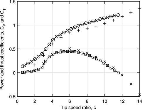
FIGURE 4. Simple model results for power (×) and thrust (+) coefficients compared to the measurements of Krogstad and Adaramola (2012) and Krogstad and Eriksen (2013).

TABLE 1

TABLE 1. Effect of a number of blade elements on power and thrust.

The two methods for calculating u are shown in Figure 5 at λ = 10, which is the closest to λ_R that measurements were made. Eq. 4 gave higher values of u across the rotor, so these were used to compute C_P and C_T. These should be lower than the values measured one radius downwind by an amount that is difficult to estimate. It is, however, noteworthy that the high values near the edge of the rotor have been reproduced, at least qualitatively. There is considerable discrepancy between the two calculations of u toward the hub, and it is likely that the large negative values are unphysical. They result from helical symmetry, which forces u to have the same sign as w and Γ. Furthermore, it is not clear whether zero or slightly negative u measured downwind of the rotor and nacelle implies similar values at the rotor computed without considering the nacelle.

FIGURE 5

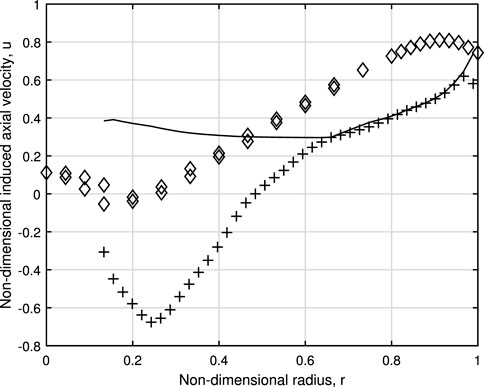
FIGURE 5. Induced axial velocity through the rotor at λ = 10. Eq. 4 after Eq. 10 was solved for w with $\overline{u^2}-\overline{v^2}=0$, solid line, from helical symmetry, +. Measurements of Krogstad and Adaramola (2012) and Krogstad and Eriksen (2013), ♢ taken in a vertical traverse through the wake, one rotor radius downwind of the rotor. They have been converted to radial profiles.

Negative w indicates that a part of the rotor is operating as a propeller, whose flow normally contracts by a small amount rather than expanding significantly. In the present case, the “propeller region” is near the hub where we would expect v² to be small. Assuming v² = 0 and including u² in the MT calculation forces u = 0. This can be seen by starting with

$\frac{dQ}{d{T}_{*}}=r\tan \varphi =r\frac{1-u}{w+\lambda r}=p,(12)$

where the first equality comes from dividing the BE part of Eq. 4 by that of Eq. 10 and the second from the blade element velocity triangle in Figure 1. Alternatively, using the right sides of Eqs 4, 10 with v² = 0 gives

$\frac{dQ}{d{T}_{*}}=r\frac{1-u}{w+\lambda r-u^2/w},(13)$

and so u = 0 for consistency. If u is set to zero in the BEMT calculations whenever w < 0, C_P, C_T, and λ_R increase; at λ = 12, for example, C_P increases to 0.248, C_T to 1.405, and λ_R to be closer to 14. The change is largely due to the reduction in magnitude of the negative w value, which is not shown. Detailed measurements of all velocity components emerging from the rotor would be a valuable aid for improving the modeling. The development of the calculated induced velocities (without setting u = 0 for negative w) with λ is shown in Figure 6. At λ_opt, w is everywhere positive but has a propeller region by λ = 10. The figure suggests the discrepancy between the two methods of determining u becomes more important as λ increases, and there is an increasing part of the rotor where w and Γ are negative. It appears that the runaway is approached more by the overall rotor torque going to zero rather than the torque on all elements being zero. This is consistent with the development of the vortex pitch shown in Figure 7). p decreases with λ, but the very small value at the runaway from Eq. 11 is confined to the tip region.

FIGURE 6

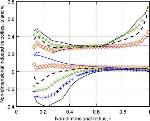
FIGURE 6. Simple model results for the induced axial and circumferential velocities for the values of λ: 4, blue solid line; 6, red ♢; 8, dashed black line; 10, green×; 12, blue +; and 14, solid black line. Note that u increases with λ near the hub from a minimum just below 0.2, but w decreases and that u for λ = 12 is not plotted.

FIGURE 7

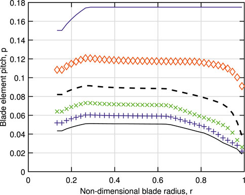
FIGURE 7. Simple model results for the vortex pitch. Symbols as in Figure 6.

4 Discussion and conclusion

The comparison with the experimental results in the previous section shows that the wake vorticity term in the revised BEMT provides a plausible explanation for the occurrence of a runaway as a consequence of the blade element drag, and a reasonable description of the λ − dependence of the thrust and power as the runaway is approached. In addition, the high values of the calculated induced axial velocity near the blade tip as the runaway is approached agree qualitatively with the experiment. These high values arise from the effective decoupling of the thrust from the axial velocity through the wake vorticity term which we added to BEMT.

What is not clear is whether the particular form of the wake vorticity term is sufficient, and ignoring the effects of the shed vorticity is justified. The thrust is consistently under-predicted (Figure 4), suggesting that additional shed vorticity terms are needed in the axial momentum equation, as argued by Limacher et al. (2022). We also note that Ebert and Wood (2002) found the tip vortex had sufficient negative angular momentum at runaway to balance the kinetic energy deficit in the remainder of the wake. If this is a general feature, then the angular momentum equation would require revision. Figure 6 shows that the wake considered here had a substantial deficit in kinetic energy at runaway, which must be balanced elsewhere in the wake to prevent it from being extracted by the rotor. It will be necessary to explore the link between this balance and the wake vorticity term before the revision of BEMT can be completed. This would require measurements of the three-dimensional distribution of all three velocity and vorticity components immediately behind the rotor—a task that is far from trivial.

Runaway at high λ may be associated with the blade element lift and drag changing from the two-dimensional values used here. There is a long history of three-dimensional corrections to airfoil data, e.g., Bangga et al. (2023), which should be investigated in future experiments. On the other hand, high λ is likely to reduce the effective blade sweep caused by the large v velocities as the rotor flow expands significantly.

A further issue is a consequence of the large u value; the expansion integral in Eq. 2 requires high levels of the radial velocity, v, near runaway. The calculations of Wood and Limacher (2021) suggest that v is smaller than u near the axis of rotation where v must be zero. v is then comparable to u near the blade tip and greater in the external flow. In the present context, this suggests a complex wake development. On the other hand, it is emphasized that the simple revision to BEMT is based on using a control volume for the axial and angular momentum equations that ends immediately behind the blades. Thus, no relation between the axial velocity leaving the rotor and in the far-wake is required. Because the angular and axial momentum fluxes must be constant downwind of the turbine, there are only two ways the wake can influence the present model: in determining the spanwise variations induced by its vorticity distribution and through the shed vorticity as noted previously. Gupta and Leishman (2005) imply that the wake at high λ (small p) becomes unstable, and this results in the so-called “vortex ring” and “turbulent wake” states and the breakdown of BEMT. The importance of the wake vorticity term suggests otherwise, unless large amounts of radial vorticity are associated with these states. This seems unlikely, however, as the “free wake” model of Gupta and Leishman (2005) does not include the radial vorticity associated with the blade drag. The complexity of the wake at high thrust is also suggested by the simulations of Martínez-Tossas et al. (2022) but again without considering the effect of the wake vorticity term.

Two general aspects of the wake vorticity term and the current analysis are worth mentioning. Eq. 12 gives the vortex pitch as the ratio of the blade element torque to reduced thrust, which also holds for the ideal actuator disc model of Wood and Hammam (2022), for which dT = dT*. Thus, it is not surprising that the runaway is associated with p ↓ 0. Second, the circulation is found from the axial momentum equation, which has significant contributions from the blade element drag. It follows that blade element circulation, in general, is determined partly by drag. This is also a consequence of the angular momentum (Eq. 4) having no wake vorticity term to cancel the drag. A similar result holds for elements of a cascade (Golmirzaee and Wood, 2023).

In conclusion, it is clear that there is still much to learn about wind turbine operation in the high-thrust region. Detailed and high-quality experiments are needed to guide the further development of models for numerical simulation. The present contribution suggests the wake vorticity term in the axial momentum equation will be an important part of improved models.

Data availability statement

The raw data supporting the conclusion of this article will be made available by the authors, without undue reservation.

Author contributions

DW: conceptualization, formal analysis, funding acquisition, investigation, methodology, resources, software, supervision, and writing-original draft. NG: conceptualization, formal analysis, and writing-original draft.

Funding

The authors declare financial support was received for the research, authorship, and/or publication of this article. This work was supported by the NSERC Discovery Grant RGPIN/04886-2017 and the Schulich endowment to the University of Calgary.

Acknowledgments

The authors are grateful to Drs Jan Bartl and Per-Å ge Krogstad for tabulations of their experimental results that were used here.

Conflict of interest

The authors declare that the research was conducted in the absence of any commercial or financial relationships that could be construed as a potential conflict of interest.

Publisher’s note

All claims expressed in this article are solely those of the authors and do not necessarily represent those of their affiliated organizations, or those of the publisher, the editors, and the reviewers. Any product that may be evaluated in this article, or claim that may be made by its manufacturer, is not guaranteed or endorsed by the publisher.

References

Bangga, G., Parkinson, S., and Lutz, T. (2023). Utilizing high fidelity data into engineering model calculations for accurate wind turbine performance and load assessments under design load cases. IET Renew. Power Gener. 17, 2909–2933. doi:10.1049/rpg2.12649

CrossRef Full Text | Google Scholar

Bartl, J., Sagmo, K. F., Bracchi, T., and Sætran, L. (2019). Performance of the nrel s826 airfoil at low to moderate Reynolds numbers—A reference experiment for cfd models. Eur. J. Mechanics-B/Fluids 75, 180–192. doi:10.1016/j.euromechflu.2018.10.002

CrossRef Full Text | Google Scholar

Ebert, P., and Wood, D. (2002). The near wake of a model horizontal-axis wind turbine at runaway. Renew. Energy 25, 41–54. doi:10.1016/s0960-1481(01)00011-8

CrossRef Full Text | Google Scholar

Golmirzaee, N., and Wood, D. H. (2023). Investigating horizontal axis wind turbine aerodynamics using cascade flows. J. Renew. Sustain. Energy 15, 043302. doi:10.1063/5.0147946

CrossRef Full Text | Google Scholar

Gupta, S., and Leishman, J. (2005). “Comparison of momentum and vortex methods for the aerodynamic analysis of wind turbines,” in 43rd AIAA aerospace sciences meeting and exhibit, 594. doi:10.2514/6.2005-594

CrossRef Full Text | Google Scholar

John, I. H., Wood, D. H., and Vaz, J. R. (2023). Helical vortex theory and blade element analysis of multi-bladed windmills. Wind Energy 26, 228–246. doi:10.1002/we.2796

CrossRef Full Text | Google Scholar

Krogstad, P.-Å., and Adaramola, M. S. (2012). Performance and near wake measurements of a model horizontal axis wind turbine. Wind Energy 15, 743–756. doi:10.1002/we.502

CrossRef Full Text | Google Scholar

Krogstad, P.-Å., and Eriksen, P. E. (2013). Blind test calculations of the performance and wake development for a model wind turbine. Renew. Energy 50, 325–333. doi:10.1016/j.renene.2012.06.044

CrossRef Full Text | Google Scholar

Limacher, E. J., Ding, L., Piqué, A., Smits, A. J., and Hultmark, M. (2022). On the relationship between turbine thrust and near-wake velocity and vorticity. J. Fluid Mech. 949, A24. doi:10.1017/jfm.2022.722

CrossRef Full Text | Google Scholar

Limacher, E. J., and Wood, D. H. (2021). An impulse-based derivation of the Kutta–Joukowsky equation for wind turbine thrust. Wind Energ. Sci. 6, 191–201. doi:10.5194/wes-6-191-2021

CrossRef Full Text | Google Scholar

Liu, L. Q., Zhu, J. Y., and Wu, J. Z. (2015). Lift and drag in two-dimensional steady viscous and compressible flow. J. Fluid Mech. 784, 304–341. doi:10.1017/jfm.2015.584

CrossRef Full Text | Google Scholar

Martínez-Tossas, L. A., Branlard, E., Shaler, K., Vijayakumar, G., Ananthan, S., Sakievich, P., et al. (2022). Numerical investigation of wind turbine wakes under high thrust coefficient. Wind Energy 25, 605–617. doi:10.1002/we.2688

CrossRef Full Text | Google Scholar

Pratumnopharat, P., and Leung, P. S. (2011). Validation of various windmill brake state models used by blade element momentum calculation. Renew. Energy 36, 3222–3227. doi:10.1016/j.renene.2011.03.027

CrossRef Full Text | Google Scholar

Sarlak, H., Nishino, T., Martínez-Tossas, L., Meneveau, C., and Sørensen, J. N. (2016). Assessment of blockage effects on the wake characteristics and power of wind turbines. Renew. Energy 93, 340–352. doi:10.1016/j.renene.2016.01.101

CrossRef Full Text | Google Scholar

Schmitz, S. (2020). Aerodynamics of wind turbines: A physical basis for analysis and design. John Wiley and Sons.

Google Scholar

Sessarego, M., Dixon, K., Rival, D., and Wood, D. (2015). A hybrid multi-objective evolutionary algorithm for wind-turbine blade optimization. Eng. Optim. 47, 1043–1062. doi:10.1080/0305215x.2014.941532

CrossRef Full Text | Google Scholar

Spera, D. A. (1994). Wind turbine technology (Fairfield, NJ (United States). American Society of Mechanical Engineers.

Google Scholar

Wood, D., and Hammam, M. (2022). Optimal performance of actuator disc models for horizontal-axis turbines. Front. Energy Res. 10, 1673. doi:10.3389/fenrg.2022.971177

CrossRef Full Text | Google Scholar

Wood, D. H., and Limacher, E. J. (2021). Some effects of flow expansion on the aerodynamics of horizontal-axis wind turbines. Wind Energy Sci. 6, 1413–1425. doi:10.5194/wes-6-1413-2021

CrossRef Full Text | Google Scholar

Wood, D., Okulov, V., and Bhattacharjee, D. (2016). Direct calculation of wind turbine tip loss. Renew. Energy 95, 269–276. doi:10.1016/j.renene.2016.04.017

CrossRef Full Text | Google Scholar

Wood, D., Okulov, V., and Vaz, J. (2021). Calculation of the induced velocities in lifting line analyses of propellers and turbines. Ocean. Eng. 235, 109337. doi:10.1016/j.oceaneng.2021.109337

CrossRef Full Text | Google Scholar

Wood, D. (2011). Small wind turbines: Analysis, design, and application. 1st edn. England: Springer London.

Google Scholar

Wood, D. (2021). Wake expansion and the finite blade functions for horizontal-axis wind turbines. Energies 14, 7653. doi:10.3390/en14227653

CrossRef Full Text | Google Scholar

Wu, J.-Z., Ma, H.-Y., and Zhou, M.-D. (2015). Vortical flows. Springer.

Google Scholar

Glossary