Short-term interval prediction of PV power based on quantile regression-stacking model and tree-structured parzen estimator optimization algorithm

In recent years, the photovoltaic (PV) industry has grown rapidly and the scale of grid-connected PV continues to increase. The random and fluctuating nature of PV power output is beginning to threaten the safe and stable operation of the power system. PV power interval forecasting can provide more comprehensive information to power system decision makers and help to achieve risk control and risk decision. PV power interval forecasting is of great importance to power systems. Therefore, in this study, a Quantile Regression-Stacking (QR-Stacking) model is proposed to implement PV power interval prediction. This integrated model uses three models, extreme gradient boosting (Xgboost), light gradient boosting machine (LightGBM) and categorical boosting (CatBoost), as the base learners and Quantile Regression-Long and Short Term Memory (QR-LSTM) model as the meta-learner. It is worth noting that in order to determine the hyperparameters of the three base learners and one meta-learner, the optimal hyperparameters of the model are searched using a Tree-structured Parzen Estimator (TPE) optimization algorithm based on Bayesian ideas. Meanwhile, the correlation coefficient is applied to determine the input characteristics of the model. Finally, the validity of the proposed model is verified using the actual data of a PV plant in China.

1 Introduction

In recent years, the human demand for electrical energy has been increasing. At present, thermal power generation occupies 60% of the global electricity energy supply, however, thermal power generation requires a large amount of non-renewable energy in the production process, and the non-renewable energy sources stored on the Earth, such as coal, oil and natural gas, are becoming increasingly depleted (Viet et al., 2020), and the energy crisis has sounded an alarm for mankind for mankind (Frilingou et al., 2023). Therefore, accelerate the energy revolution, optimize the energy structure is urgent to achieve sustainable development of energy has become a key concern of countries around the world. Solar energy is a renewable energy source with great potential, and countries around the world have reached a consensus on the need for solar energy development, of which photovoltaic power generation is an important way of solar energy development and utilization (Rafique et al., 2020; Khalid et al., 2023). With the progress of technology and cost reduction, photovoltaic power generation has been widely promoted and applied in all countries around the world, and the installed capacity has been rising in recent years.

PV power output is uncontrollable and subject to various meteorological factors, showing strong volatility, randomness, intermittency and non-smoothness. The PV power system is equivalent to an uncontrollable power source for the power system. With the increasing scale of grid-connected PV, unstable PV power output will cause difficulties in power system scheduling and real-time power balancing. At the same time, PV power output fluctuations can lead to sharp fluctuations in frequency and voltage, and the resulting shocks may threaten the safe and stable operation of the power system. In addition, large-scale grid-connected PV may have a certain negative impact on the damping characteristics of the power system, which in turn threatens the safe and stable operation of the power system (Rafique et al., 2022). Therefore, in order to improve the security of the power system and the reliability of power supply, the light has to be abandoned. Accurate PV power prediction helps the power system scheduling department to reasonably arrange the power system scheduling plan and realise the real-time balance of power generation and power consumption, so as to ensure that the power system can operate reliably, safely and stably. For PV power operating companies, it can improve the economic efficiency of PV power plants. In addition to this, energy storage technology has a very high potential in reducing the threat of PV fluctuations to the power system (Amir et al., 2023).

According to the different mechanisms within the prediction models, PV output forecasting models can be categorized into: physical models, statistical models, machine learning models and integrated models. The physical prediction model uses the installation position, tilt angle, design parameters, operating characteristics and conversion efficiency of PV modules to establish a physical model, while meteorological data such as solar irradiance is used as the data basis for the physical model to obtain the predicted value of PV power generation through the calculation of the physical model (Dolara et al., 2015). The statistical model is only data-driven. The statistical model inputs weather variables such as solar irradiance and historical data of PV power, and extracts the intrinsic correlation information to build a mapping model to achieve the prediction of future PV output (Gellert et al., 2022). While traditional statistical methods have very limited nonlinear modeling capability, machine learning prediction models (Rao et al., 2022) have powerful nonlinear mapping modeling capability, which has led to its rapid development in the field of PV forecasting. Twenty-four machine learning models were developed for implementing PV power prediction by Dávid Markovics et al. Day-ahead PV power prediction was performed based on numerical weather forecast data. The effects of predictor variable selection and the benefits of hyperparameter tuning were also investigated in detail in this study (Markovics and Mayer, 2022). In recent years many researchers have turned to the development and research work of combined prediction models (Liang et al., 2023), which have superior predictive performance, model generalization performance, and robustness.

Traditional PV power prediction techniques focus on point prediction. The output of point prediction is a single point expected value of PV power at a certain moment in the future. However, due to the chaotic nature of the atmospheric system, PV power prediction errors cannot be avoided. There are significant uncertainties in the prediction results, and the information provided by point prediction is very limited. In contrast to point prediction, interval prediction of PV power uses prediction intervals to achieve a quantitative estimate of the prediction uncertainty. The interval prediction results provide the upper and lower bounds of the fluctuation of PV power at a certain confidence level at a certain time in the future, which makes up for the limitations of the PV power point prediction technique and can provide more comprehensive data support for the power system. The PV power interval prediction results can provide important references for the operational risk assessment and risk decision-making of the power system, and further improve the security and economy of the power system. In addition, PV power interval prediction technology has a very broad application prospect in the fields of power system planning, power system scheduling, energy storage configuration and regulation, and power market trading. Zhenhao Wang et al. (Wang et al., 2022)established a deep convolutional generative adversarial network model to generate PV power characteristic curves in different scenarios, and then established a QRLSTM model to achieve PV power interval prediction. Ming Ma et al. (Ma et al., 2022)analysed the distribution of PV power prediction errors and then constructed PV power prediction intervals using a kernel density estimation algorithm.

The existing PV power interval prediction is mainly realised using a single model, and its prediction performance needs to be further improved. Multi-model fusion technology will be an important development direction in the future. The values of the model parameters largely determine the prediction performance of the model, so the hyperparameter optimisation problem of the fusion model needs further research. Therefore, in this paper a stacking model that can achieve the prediction of PV power intervals is proposed. An optimisation algorithm is used to determine the optimal hyperparameter values for this model to improve the PV power interval accuracy. In order to provide important data support for power system operation risk assessment and risk decision-making, and to further improve the safety and economy of the power system. The main contributions of this paper are as follows:

1) A novel QR-Stacking integrated model is proposed to implement PV power interval prediction. Multiple decision tree models are used as the base learners of this integrated model, and deep neural networks are used as the meta-learner of this integrated model. The QR-Stacking integrated model is constructed by combining the quantile regression model and the Stacking integrated model to achieve the PV power interval prediction. This is the first application of this stacking model in the field of PV power interval prediction.

2) To improve the prediction accuracy of the QR-Stacking integrated model, the Tree-structured Parzen Estimator algorithm was used to search for determining the hyperparameters of multiple base learners and a meta-learner.

3) Simulation analysis was conducted based on actual PV power generation data from a PV power plant in China. Multiple interval evaluation metrics were used to evaluate the prediction intervals. A comprehensive comparative analysis of the interval prediction accuracy of QR-Stacking and multiple benchmark prediction models was performed. The results show that the model can give full play to the advantages of each algorithm and improve the prediction accuracy of PV power intervals.

The rest of the paper is organized as follows: Section 2 describes the prediction models and optimization algorithms used in this paper. Section 3 describes in detail the evaluation metrics of the prediction model. Section 4 provides case studies. The prediction performance of the proposed prediction model is compared with that of several benchmark models. The accuracy of the prediction models is verified by experimental simulations. Section 5 summarizes the whole paper.

2 Methodology

Figure 1 shows the overall structure of the work in this paper. Firstly, three base learners, Xgboost, LightGBM and CatBoost, and a meta-learner, QR-LSTM, are built. The proposed QR-Stacking model is constructed from the above four models and the TPE optimisation algorithm. Secondly, the proposed model is trained and tested using real PV data. Finally, three evaluation metrics are used to compare and analyse the prediction performance of the proposed model with QR-LSTM and QR-GRU models. The nomenclature used in this paper is presented in Table 1.

FIGURE 1

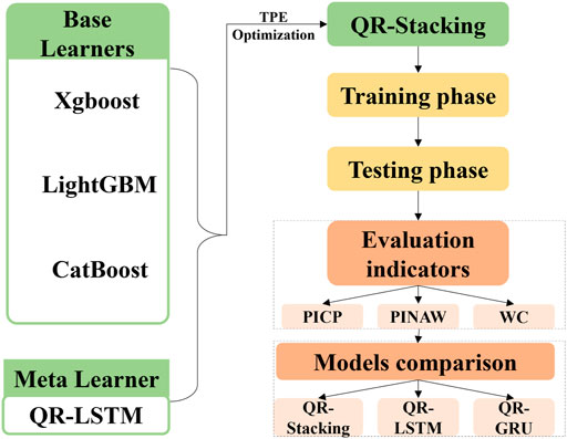
FIGURE 1. Overall structure of the work in this paper.

TABLE 1

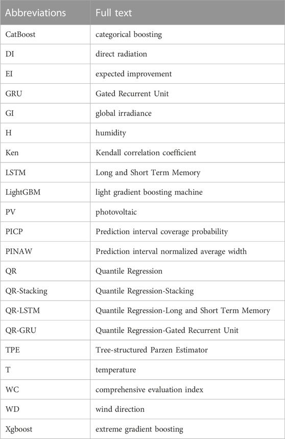
TABLE 1. Nomenclature.

2.1 Stacking

It has been shown that single prediction models have limited prediction accuracy. Ensemble machine learning would be an important solution to this challenge. Usually, the first layer of the stacking model is the base learner layer and the second layer is the meta-learner layer. The meta-learner layer corrects the prediction error of the base learner. In this research, Xgboost, LightGBM and CatBoost are used as base learners. The QR-LSTM model is used as a meta-learner. The following section details the modeling principles of the three base learners and one meta-learner.

2.2 Base learners

2.2.1 Xgboost

The XGBoost algorithm is an improved algorithm of the gradient augmented regression tree. The main improvements of the XGBoost algorithm are the improvement of the objective function and its solving method.

The objective function (loss function) of the XGBoost algorithm during training consists of two parts, as shown in Eq. 1.

$Obj={\displaystyle \sum _{i=1}^n}l(y_i,{\widehat{y}}_i)+{\displaystyle \sum _{k=1}^K}\mathrm{\Omega }\left(f_k\right)(1)$

Where ${\displaystyle \sum _{i=1}^n}l\left(y_i,{\widehat{y}}_i\right)$ is used to characterize the difference between the predicted values ${\widehat{y}}_i$ and true values $y_i$. ${\displaystyle \sum _{k=1}^K}\mathrm{\Omega }\left(f_k\right)$ is the regularization term.

The regularization term can be calculated from Eq. 2:

${\displaystyle \sum _{k=1}^K}\mathrm{\Omega }\left(f_k\right)=\gamma T+\frac{1}{2}\theta {\displaystyle \sum _{j=1}^T}{\omega }_j^2(2)$

where $\mathrm{\Omega }\left(f_k\right)$ is a function of the complexity of the decision tree $f_k$. $\gamma$ is the penalty term of the L1 regular. T is the total number of leaf nodes of the decision tree. θ is the penalty term of the L2 regular. ${\omega }_j$ is the weight of the decision tree $f_i$ at the jth leaf node.

Each iteration updates the objective function to Eq. 3.

$Ob{j}^t={\displaystyle \sum _{i=1}^n}l\left[y_i,{\widehat{y}}_i^{\left(t-1\right)}+f_t\left(x_i\right)\right]+\mathrm{\Omega }\left(f_t\right)(3)$

Using a second-order Taylor expansion for the above equation, the following equation is obtained by removing the constant term.

$Ob{j}^t={\displaystyle \sum _{i=1}^n}\left[g_i{f}_t\left(x_i\right)+\frac{1}{2}{h}_i\times f_t^2\left(x_i\right)\right]+\mathrm{\Omega }\left(f_t\right)(4)$

where $g_i={\partial }_{{\widehat{y}}_i^{\left(t-1\right)}}l\left(y_i,{\widehat{y}}_i^{\left(t-1\right)}\right)$ and $h_i={\partial }_{{\widehat{y}}_i^{\left(t-1\right)}}^{2}l\left(y_i,{\widehat{y}}_i^{\left(t-1\right)}\right)$ are the first- and second-order derivatives of the objective function, respectively.

2.2.2 LightGBM

The basic idea of LightGBM is to obtain the final strong regression tree using multiple iterations of the weak regression tree. The new regression tree obtained from each iteration is obtained by fitting the prediction residuals of the previous regression tree. Finally, the outputs of all regression trees are summed to output the better-performing results. The calculation is shown in Eq. 5.

$F\left(x\right)={\displaystyle \sum _{m=1}^M}{f}_m\left(x\right)(5)$

where $f_m\left(x\right)$ is the output value of the mth weak regression tree and $F\left(x\right)$ is the final output value of the model.

2.2.3 CatBoost

The CatBoost model is an improved gradient boosted decision tree (GBDT) model. The improvements of CatBoost over traditional GBDT are as follows:

Traditional GBDT derives the gradient of the current model based on the same dataset in each iteration of training, but this leads to biased point-by-point gradient estimation. CatBoost uses Ordered Boosting to improve the gradient estimation method of the traditional algorithm. The improved algorithm obtains an unbiased estimate of the gradient to mitigate the effect of the gradient estimation bias and thus improve the generalization ability of the model. To obtain unbiased gradient estimation, the CatBoost model trains a separate model $M_i$ for each sample $x_i$, which is obtained by training with a training set that does not contain sample $x_i$. Then $M_i$ is used to obtain a gradient estimate on the samples. Finally, this gradient is used to train the weak learner and obtain the final model.

2.3 Meta-learner

2.3.1 Quantile regression

The quantile regression (QR) model is used to study the relationship between the conditional quartiles of the independent and dependent variables. The quantile regression model can be represented by Eq. 6.

$Q_{P_i}\left(\tau |x_i\right)=x_i\beta \left(\tau \right)i=\mathrm{1,2},\cdots ,n(6)$

where $Q_{P_i}\left(\tau |x_i\right)$ is the conditional quantile. $\tau \in \left(\mathrm{0,1}\right)$. $\beta \left(\tau \right)$ is the vector of regression coefficients. $\beta \left(\tau \right)={\left[{\beta }_0\left(\tau \right),{\beta }_1\left(\tau \right),\cdots ,{\beta }_m\left(\tau \right)\right]}^T$. Each element ${\beta }_j\left(\tau \right)$ in $\beta \left(\tau \right)$ characterizes the degree of influence of the jth independent variable on the dependent variable. n is the total number of samples. $P_i$ is the dependent variable. $x_i$ is the independent variable. The dependent variable is usually multiple, i.e.,: $x_i=\left[x_{i,0},x_{i,1},\cdots ,x_{i,m}\right]$

The objective of solving the quantile regression model is $\beta \left(\tau \right)$. The problem can be solved by minimizing the loss function as shown in Eq. 7.

$L={\displaystyle \sum _{i=1}^n}{\gamma }_{\tau }\left(P_i-x_i\beta \left(\tau \right)\right)(7)$

where ${\gamma }_{\tau }$ is an asymmetric function with respect to the quantile $\tau$. $\widehat{\beta }\left(\tau \right)$ is the estimated value of $\beta \left(\tau \right)$. Its specific expression is given by:

${\gamma }_{\tau }\left(s\right)=\left\{\begin{array}{l}\tau ss\ge 0\\ \left(\tau -1\right)ss<0\end{array}\right.(8)$

where the expression of $s$ is $s=P_i-x_i\beta \left(\tau \right)$.

Thus the expression for solving $\widehat{\beta }\left(\tau \right)$ is as follows:

$\widehat{\beta }\left(\tau \right)=\mathrm{argmin}{\displaystyle \sum _{i=1}^n}{\gamma }_{\tau }\left(P_i-x_i\beta \left(\tau \right)\right)(9)$

Ultimately, the estimates obtained by quantile regression model estimation at different conditional quartiles are as follows.

${\widehat{Q}}_{P_i}\left(\tau |x_i\right)=x_i\widehat{\beta }\left(\tau \right)i=\mathrm{1,2},\cdots ,n(10)$

2.3.2 Long and Short Term Memory

The Long and Short Term Memory (LSTM) model was first proposed by Hochreiter and Schmidhuber in the 1990s as a solution to the issue of vanishing gradients in traditional RNNs. The incorporation of gating units, consisting of forgetting, input, and output gates, allows LSTMs to selectively retain or discard information within the cell state, enabling them to effectively capture and model long-term dependencies in sequential data. As a result, LSTMs have become a widely utilized tool in the field of deep learning. Figure 2 is a schematic diagram of the structure of the LSTM model.

FIGURE 2

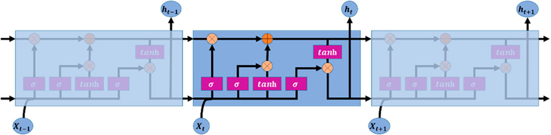
FIGURE 2. The structure of the LSTM unit.

2.3.3 Quantile Regression-Long and Short Term Memory

Quantile regression model in the form of loss function and LSTM model are fused to achieve PV power interval prediction. The Quantile Regression-Long and Short Term Memory (QR-LSTM) model serves as a meta-learner for the proposed model to further correct the prediction bias of the base learner.

2.4 Tree-structured parzen estimator

In this study, the Tree-structured Parzen Estimator (TPE) optimization algorithm is proposed to achieve the global optimization of each model hyperparameter. The TPE algorithm uses a probability density estimator based on the tree structure to implement Bayesian optimization. The TPE technique may fast converge to the global optimal solution and models the parameter space using a tree structure.

The main advantages of the TPE algorithm are (1) It avoids the inefficiencies of traditional grid search or random search by using probability density estimates to model the objective function. (Nguyen et al., 2020). (2) The TPE algorithm can automatically adjust the direction and scope of the search. (3) The TPE algorithm can handle discrete, continuous, and mixed types of hyperparameters, making it applicable to a variety of machine learning models and algorithms. (4) The TPE algorithm is based on Bayesian optimisation theory, which has a solid mathematical foundation and reliable theoretical support. (5) The TPE algorithm estimates the probability density function in the parameter space by constructing a tree-like structure, which enables it to find high probability regions quickly and reduces the size of the search space. In contrast, optimisation algorithms such as genetic algorithms require a large number of iterations and crossover operations with high computational complexity. (6) The TPE algorithm is able to handle the noise in the objective function better and find the optimal solution more stably through the estimation of the probability density function. While optimisation algorithms such as genetic algorithm may be disturbed by noise and get unstable results.

The core of TPE optimisation is to find a set of hyperparameters that minimise the established objective function. The Bayesian-based TPE optimisation algorithm reduces the number of computations and time cost by selecting the most promising set of hyperparameters for the next evaluation. Figure 3 illustrates the pseudo-code of the TPE optimisation algorithm. The following section describes in detail the selection criteria for the objective function and the next set of hyperparameters:

FIGURE 3

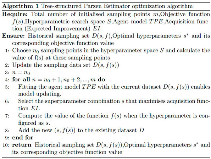
FIGURE 3. Pseudo-code of the TPE optimisation algorithm.

The goal of hyperparameter optimization is to find the value of the hyperparameter that minimizes the loss of the machine learning model. It can be expressed as Eq. 11.

$s^{*}=\underset{s\in S}{\mathit{argmin}}f\left(s\right)(11)$

where S is the optional hyperparameter space and s* is the best set of hyperparameters.

The whole concept of Bayesian optimization is to reduce the number of computations and time cost by selecting the most promising set of hyperparameters as possible for the next evaluation. The selection criteria for the next set of hyperparameters is the expected improvement (EI), which is expressed as:

$E{I}_{t^{*}}\left(s\right)={\int }_{-\infty }^{t^{*}}\left(t^{*}-t\right)p\left(t,s\right)dt(12)$

where $t^{*}$ is the threshold of the objective function, $s$ is the proposed hyperparameter, $t$ is the actual value of the objective function when the proposed hyperparameter $s$ is used, and $p\left(t,s\right)$ denotes the agent probability model.$p\left(t,s\right)$ is defined in the TPE method, and $p\left(t,s\right)$ is denoted as

$p\left(t,s\right)=\left\{\begin{array}{c}l\left(s\right)ift<t^{*}\\ g\left(s\right)ift>t^{*}\end{array}\right.(13)$

where $l\left(s\right)$ denotes the probability of hyperparameter set s when the value of the objective function $t$ is less than a threshold value $t^{*}$, $g\left(s\right)$ denotes the probability of hyperparameter set s when the value of the objective function $t$ is greater than a threshold value $t^{*}$.

The EI criteria when using the TPE method can be expressed as follows.

$E{I}_{t^{*}}\left(s\right)={\int }_{-\infty }^{t^{*}}\left(t^{*}-t\right)p\left(t,s\right)dt={\int }_{-\infty }^{t^{*}}\left(t^{*}-t\right)\frac{p\left(s,t\right)p\left(t\right)}{p\left(s\right)}dt(14)$

$p\left(s\right)$ can be denoted as $p\left(s\right)={\int }_{R}p\left(s|t\right)p\left(t\right)dt=gl\left(s\right)+\left(1-g\right)g\left(s\right)$.Let $\gamma =p\left(t<t^{*}\right)$. The final EI can be expressed as follows.

$E{I}_t^{*}\left(s\right)=\frac{\gamma t^{*}l\left(s\right)-l\left(s\right){\int }_{-\infty }^{t^{*}}p\left(t\right)dt}{\gamma l\left(s\right)+\left(1-\gamma \right)g\left(s\right)}\propto {\left(\gamma +\frac{g\left(s\right)}{l\left(s\right)}\left(1-\gamma \right)\right)}^{-1}(15)$

In order to maximize EI, the ratio $\frac{l\left(s\right)}{g\left(s\right)}$ should be maximized. Therefore, the expected set of hyperparameters s has a higher probability under $l\left(s\right)$.

Eventually, through continuous iteration, the set of hyperparameters that can make the objective function achieve the minimum value is obtained. This set of hyperparameters is the best hyperparameters for the proposed model.

2.5 Quantile regression-stacking model optimized using the tree-structured parzen estimator algorithm for photovoltaic power interval prediction

In this study a stacking model using an efficient hyperparametric optimization method for PV power interval prediction is proposed. Xgboost, LightGBM and CatBoost are used as the base learners. QR-LSTM is used as a meta-learner. Firstly, three basic learners are used to independently make predictions of PV power output, which are able to learn the trend of PV power from historical data. Each basic learner produces a set of predictions. Then, the prediction results of these base learners are fed into QR-LSTM to achieve the final prediction. QR-LSTM further corrects the prediction errors of the three base learners to improve the prediction accuracy. Notably, the quantile regression model in the QR-LSTM model is capable of constructing prediction intervals to quantify the uncertainty in PV power prediction. By combining the strengths of these learners, the QR-Stacking model is able to better address the challenges associated with PV power output fluctuations and more accurately quantify the uncertainty in PV power forecasts. In addition to this, the TPE algorithm is also used to search for the optimal parameters of the base and meta learners to further improve the interval prediction performance of the model.

The proposed stacking model is illustrated separately in a training phase and a testing phase.

2.5.1 Training phase

The steps of the stacked model training phase are shown in Figure 4. The pseudo-code for the training phase of the proposed model is presented in Figure 5. The 5-fold cross-validation and TPE parameter optimization methods are used in the training phase of the proposed stacking model. The details are illustrated below.

1) The training set is divided into 5 folds.

2) Training the Xgboost model using a 5-fold cross-validation method and a TPE parameter optimization method. In the first iteration, the last 4 folds are used for training the model and the first fold is used for prediction. The obtained prediction result is $P_{Xgboost}^{1-fold}$. In the second iteration, the second fold is used for prediction and the remaining four folds are used for training. The obtained prediction result is $P_{Xgboost}^{2-fold}$. This process is repeated until the prediction results are obtained for all 5 folds. Finally, the prediction result obtained by the Xgboost model is:

$P_{Xgboost}^{Train}=\left[P_{Xgboost}^{1-fold},P_{Xgboost}^{2-fold},P_{Xgboost}^{3-fold},P_{Xgboost}^{4-fold},P_{Xgboost}^{5-fold}\right](16)$

3) Using the same process as (16), the outputs obtained from the LightGBM and CatBoost models are expressed as follows.

$P_{LightGBM}^{Train}=\left[P_{LightGBM}^{1-fold},P_{LightGBM}^{2-fold},P_{LightGBM}^{3-fold},P_{LightGBM}^{4-fold},P_{LightGBM}^{5-fold}\right](17)$

$P_{CatBoost}^{Train}=\left[P_{CatBoost}^{1-fold},P_{CatBoost}^{2-fold},P_{CatBoost}^{3-fold},P_{CatBoost}^{4-fold},P_{CatBoost}^{5-fold}\right](18)$

4) The prediction results of the three base learners are merged to obtain a new training set $P_{New}^{Train}$. The matrix $P_{New}^{Train}$ and the original dependent variable $P_{Original}^{Train}$ are used as training data for the meta-learner.

$P_{New}^{Train}=\left[\begin{array}{ccc}{P}_{Xgboost}^{1-fold}& P_{LightGBM}^{1-fold}& P_{CatBoost}^{1-fold}\\ P_{Xgboost}^{2-fold}& P_{LightGBM}^{2-fold}& P_{CatBoost}^{2-fold}\\ P_{Xgboost}^{3-fold}& P_{LightGBM}^{3-fold}& P_{CatBoost}^{3-fold}\\ P_{Xgboost}^{4-fold}& P_{LightGBM}^{4-fold}& P_{CatBoost}^{4-fold}\\ P_{Xgboost}^{5-fold}& P_{LightGBM}^{5-fold}& P_{CatBoost}^{5-fold}\end{array}\right](19)$

5) The dimension of matrix $P_{New}^{Train}$ is transformed into three dimensions to satisfy the QR-LSTM model input requirements, and the new matrix $P_{New\_1}^{Train}$ is obtained. The prediction results $P_{New\_1}^{Train}$ of the base learners and the training set $P_{Original}^{Train}$ of the dependent variable are fed to the meta-learner QR-LSTM for training. It is worth noting that the meta-learner also uses the TPE algorithm for parameter optimization to exploit its optimal predictive performance.

FIGURE 4

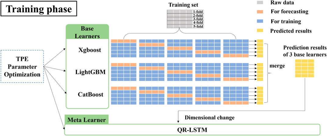
FIGURE 4. Flow chart of the training phase of the proposed stacking model.

FIGURE 5

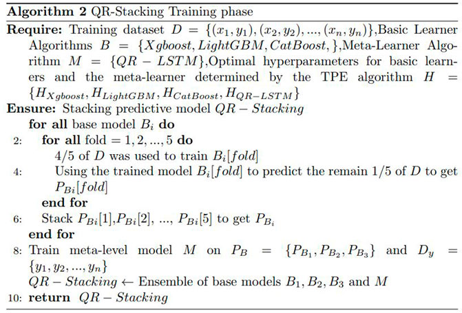
FIGURE 5. Pseudo-code for the training phase of the proposed model.

2.5.2 Testing phase

The detailed flow of the testing phase is shown in Figure 6. The pseudo-code for the testing phase of the proposed model is presented in Figure 7. In the testing phase, the test dataset is fed into the stacking model to implement PV power interval prediction. It is worth mentioning that the cross-validation strategy is no longer used in the testing phase and an average strategy is introduced to deal with the multiple predictions of each base learner. The details are described as follows.

1) The test set is fed to each base learner for prediction. A 5-fold cross-validation strategy is used in the training phase, hence for each base learner five different models are generated after training. Therefore, each base learner is capable of obtaining five predictions. The prediction results of each model are as follows.

$P_{Xgboost}^{Test}=\left[P_{Xgboost}^{Test\_1},P_{Xgboost}^{Test\_2},P_{Xgboost}^{Test\_3},P_{Xgboost}^{Test\_4},P_{Xgboost}^{Test\_5}\right](20)$

$P_{LightGBM}^{Test}=\left[P_{LightGBM}^{Test\_1},P_{LightGBM}^{Test\_2},P_{LightGBM}^{Test\_3},P_{LightGBM}^{Test\_4},P_{LightGBM}^{Test\_5}\right](21)$

$P_{CatBoost}^{Test}=\left[P_{CatBoost}^{Test\_1},P_{CatBoost}^{Test\_2},P_{CatBoost}^{Test\_3},P_{CatBoost}^{Test\_4},P_{CatBoost}^{Test\_5}\right](22)$

2) The 5 predictions of each base learner are averaged and 3 new matrices are obtained:

$P_{Xgboost}^{Test-New}=\frac{1}{5}{\displaystyle \sum _{i=1}^5}{P}_{Xgboost}^{Test\_i},P_{LightGBM}^{Test-New}=\frac{1}{5}{\displaystyle \sum _{i=1}^5}{P}_{LightGBM}^{Test\_i},P_{CatBoost}^{Test-New}=\frac{1}{5}{\displaystyle \sum _{i=1}^5}{P}_{CatBoost}^{Test\_i}$

.

3) The 3 matrices are combined and used as feed-in data for the meta-learner. The matrix obtained by merging the matrices is: $P_{Merge}^{Test}$.

$P_{Merge}^{Test}=\left[P_{Xgboost}^{Test-New},P_{LightGBM}^{Test-New},P_{CatBoost}^{Test-New}\right](23)$

4) The matrix $P_{Merge}^{Test}$ is dimensionally transformed and fed into a QR-LSTM model to achieve PV power interval prediction. PV power prediction results under different quartiles are obtained. The predicted result is $W_i=\left[{\widehat{Q}}_{P_i}\left({\tau }_1|x_i\right),{\widehat{Q}}_{P_i}\left({\tau }_2|x_i\right),\dots ,{\widehat{Q}}_{P_i}\left({\tau }_L|x_i\right)\right]$.

FIGURE 6

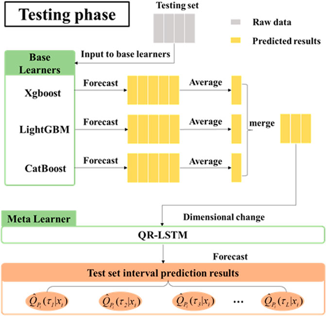
FIGURE 6. Flow chart of the testing phase of the proposed stacking model.

FIGURE 7

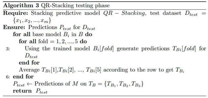
FIGURE 7. Pseudo-code for the testing phase of the proposed model.

3 Evaluation indicators for interval prediction results

Prediction Interval Coverage Probability (PICP) is an important statistic for assessing prediction interval reliability, and a larger value implies that the model predicts a more trustworthy interval. Prediction interval normalized average width (PINAW) is an essential statistic for assessing prediction interval accuracy, and a lower value suggests that the model predicts a more accurate interval. There is a relationship between PICP and PINAW. In general, the higher the PICP, the lower the PINAW, indicating that the model is more confident in the prediction interval. Simultaneously, there is a contradictory link between PICP and PINAW. When the prediction interval is large, it is easy to attain high interval coverage probability. However, prediction intervals that are too wide cannot provide accurate uncertainty information.

PINAW, PICP and WC indicators are calculated based on Eq. 24 (25) (26), respectively:

$PICP=\left(1/N\right)·{\displaystyle \sum _{n=1}^N}{S}_n(24)$

where N denotes the number of data. $S_n$ represents a Boolean function. The value of this Boolean function takes 1 when the prediction interval of the model contains the true value, otherwise, it is 0.

$PINAW=\left[1/\left(N·E\right)\right]·{\displaystyle \sum _{n=1}^N}\left(P_{up}-P_{down}\right)(25)$

where N is the total number of data. E denotes the difference between the maximum and minimum values of PV power. $P_{up}$ and $P_{down}$ respectively represent the upper and lower bound of the interval prediction.

There is a conflicting relationship between PICP and PINAW. Therefore, by combining these two indicators, a comprehensive evaluation index is proposed. The comprehensive evaluation index (WC) is calculated using Eq. 26. The smaller the WC value, the more superior the interval obtained.

$WC=PINAW/PICP(26)$

4 Case studies

4.1 Data sets

The data used in this study are from a photovoltaic power plant in Hebei, China. The dataset is sampled at 15-min intervals. The historical data set includes active power (P), global irradiance (GI), direct radiation (DI), temperature (T), humidity (H), wind speed (WS), wind direction (WD), and pressure (P). Most of the nighttime zero-value data were removed in this study.

4.2 Selection of model input features

It is well known that PV power output is very closely related to several meteorological factors. In order to improve the accuracy of PV power prediction, it is usually necessary to filter several meteorological variables to get the meteorological variables that show high correlation with PV power output. In this study, the Kendall correlation coefficient was used for variable correlation analysis.

The Kendall correlation coefficient is calculated as follows:

$Ken=\frac{P-Q}{\raisebox{1ex}{$1$}\!\left/ \!\raisebox{-1ex}{$2$}\right.*N*\left(N-1\right)}(27)$

where P and Q denote the number of harmonious and discordant quantities, respectively. The denominator of the formula indicates the total number of pairs of observations.

For comparison and analysis, a heat map was drawn based on the calculated Kendall correlation coefficients, as shown in Figure 8. The numbers in this figure characterise the degree of correlation between the variables. Numbers closer to 1 indicate a higher degree of correlation, and numbers closer to 0 indicate a lower degree of correlation. A negative number indicates a negative correlation.

FIGURE 8

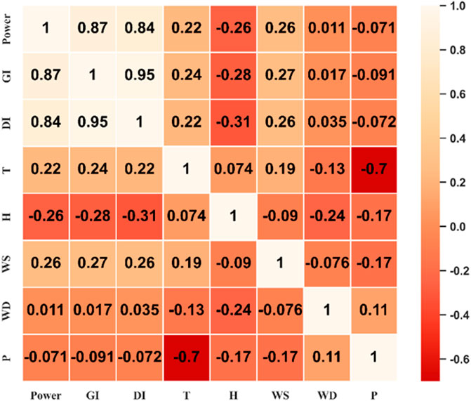
FIGURE 8. Heat map of correlation between power variables and meteorological factor variables.

Figure 8 shows that global irradiance (GI), direct radiation (DI), wind direction (WD), temperature (T) and humidity(H) are the main meteorological variables affecting PV output, so these five variables are chosen as input variables for the model.

4.3 Model parameter setting and data set division

The hyperparameter search range settings for the base learners and meta-learner are shown in Table 2. The LSTM model consists of one layer of LSTM network layer, one layer of Dropout layer, and one layer of Dense layer. The number of neurons of the LSTM network layer, the dropout rate, and the activation function of the Dense layer are optimized. The number of neurons in the Dense layer is 199, i.e., the quantile takes a range of values from 0.005 to 1, and the step size is 0.005.The optimizer for LSTM model training is adam, and the batch_size is 48. The epochs for the training of the LSTM model are set to 150 and an early stopping strategy is used to avoid the overfitting problem. Each base learner uses a decision tree model, which runs faster, so its hyperparameter search time is set to 200 s. The number of hyperparameter searches for the meta-learner model is 100.

TABLE 2

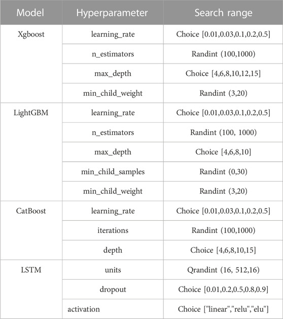
TABLE 2. The hyperparameter search range settings for the base learners and meta-learner.

The ratio of training set, validation set and test set was 7:2:1. 100 days of data were used in this study. One sunny day and one rainy day in the test set were selected separately for each model performance comparison. The model output is the predicted PV power for the 199 quantile points of the future day. The prediction interval is constructed by selecting several of the quantile predictions.

4.4 Predictive performance comparison

In order to evaluate the prediction performance of the proposed QR-Stacking model, two benchmark models and the QR-Stacking model are developed in this paper for prediction performance comparison. The two benchmark models established in this paper are QR-LSTM and Quantile Regression-Gated Recurrent Unit (QR-GRU). In order to make a valid comparison, the benchmark models QR-LSTM and QR-GRU also use the TPE algorithm for parameter search. The search parameter setting ranges of the benchmark models QR-LSTM and QR-GRU are kept the same as those of the QR-Stacking model. To verify the generalization performance of the models, the prediction performance of the three models under several different weather conditions is compared and analyzed. It is worth noting that the prediction performance of each model is compared at 95%, 90% and 85% confidence levels in this study.

4.4.1 Comparison of the prediction performance of the models during sunny days

The prediction intervals of the three models under sunny conditions are shown in Figures 9, 10, and 11. Figures 9, 10, and 11 show that the proposed QR-Stacking model has the highest interval coverage and narrow interval width.

FIGURE 9

FIGURE 9. Forecast intervals of the QR-Stacking model during sunny days.

FIGURE 10

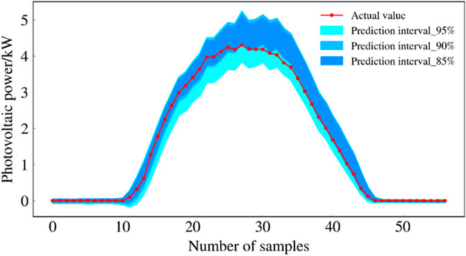
FIGURE 10. Forecast intervals of QR-LSTM model during sunny days.

FIGURE 11

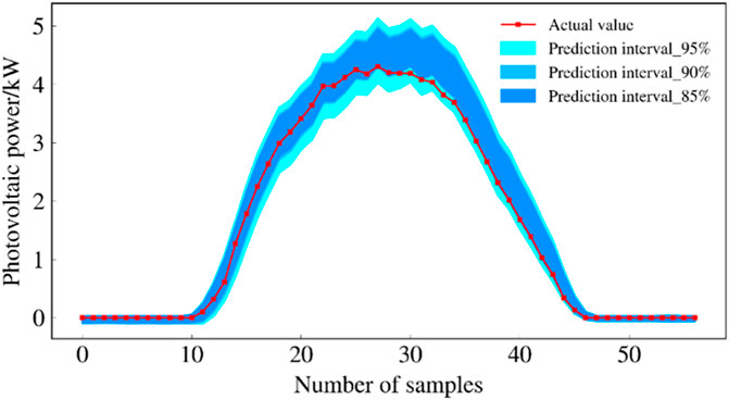
FIGURE 11. Forecast intervals of QR-GRU model during sunny days.

Table 3 evaluates the prediction interval of each model at three confidence levels using several evaluation metrics. The prediction interval coverage of all three models at 95% confidence level can meet the requirements, i.e., the coverage rate is greater than 95%. However, the prediction interval coverage of the QR-LSTM and QR-GRU models at 90% and 85% confidence levels cannot meet the requirements. In terms of PINAW and WC metrics, the prediction interval of QR-Stacking model can provide narrower prediction intervals while meeting the interval coverage requirement. At the 95% confidence level, the WC indicator of the prediction interval of the QR-Stacking model is 11.02% and 3.21% lower than those of the QR-LSTM and QR-GRU models, respectively. The WC metrics of the prediction intervals of the QR-Stacking model are 6.54% and 6.93% lower than those of the QR-LSTM and QR-GRU models, respectively, at the 90% confidence level. At the 85% confidence level, the WC metrics of the prediction intervals of the QR-Stacking model are 2.92% and 10.73% lower than those of the QR-LSTM, and QR-GRU models, respectively.

TABLE 3

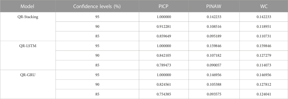
TABLE 3. Evaluation of the prediction results of each model during sunny days.

In summary, the prediction interval of the QR-Stacking model is best in sunny days.

4.4.2 Comparison of prediction performance of various models during rainy days

The prediction intervals of the three models for cloudy and rainy days are shown in Figures 12, 13 and 14. These three plots show that the prediction interval coverage of the proposed model meets the requirements and the interval is narrower.

FIGURE 12

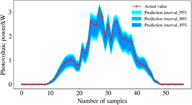
FIGURE 12. Forecast intervals of QR-Stacking model during rainy days.

FIGURE 13

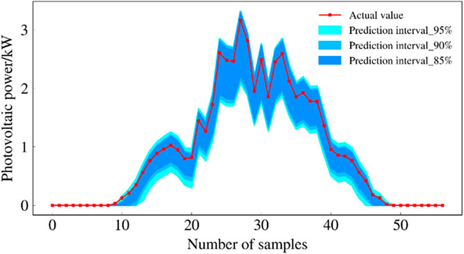
FIGURE 13. Forecast intervals of QR-LSTM model during rainy days.

FIGURE 14

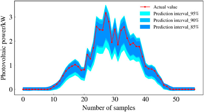
FIGURE 14. Forecast intervals of QR-GRU model during rainy days.

Table 4 evaluates the prediction intervals of each model at three confidence levels using multiple evaluation metrics. The prediction interval coverage of the 3 models can meet the requirements of each confidence level. In terms of PINAW and WC metrics, the prediction interval of QR-Stacking model can provide narrower prediction intervals while meeting the interval coverage requirement. At the 95% confidence level, the WC indicator of the forecast results of the QR-Stacking model is 11.06% and 23.72% lower than those of the QR-LSTM and QR-GRU models, respectively. At the 90% confidence level, the WC metrics of the prediction interval of the QR-Stacking model are 18.38% and 23.10% lower than those of the QR-LSTM and QR-GRU models, respectively. At the 85% confidence level, the WC metrics of the prediction interval of the QR-Stacking model are 21.41% and 24.11% lower than those of the QR-LSTM, QR-GRU models, respectively.

TABLE 4

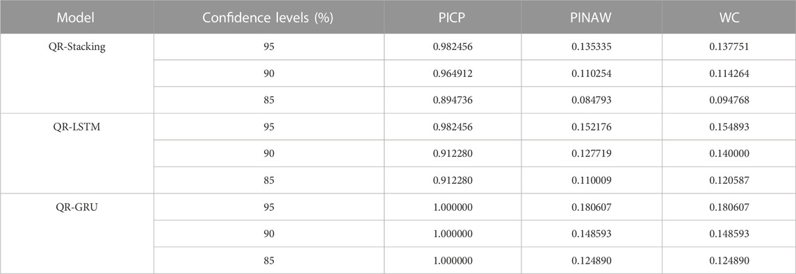
TABLE 4. Evaluation of prediction results of each model during cloudy and rainy days.

In summary, the QR-Stacking model has the best prediction interval during cloudy and rainy days.

5 Conclusion

In this research, a QR-Stacking model with hyperparameter optimization using TPE algorithm is proposed to improve the reliability and acuity of PV power interval prediction. The conclusions are stated as follows:

1) Kendall correlation coefficient is used to screen several meteorological features. This method removes the redundant features of the input data and reduces the complexity of the model.

2) QR-Stacking model has more superior interval prediction performance than the two benchmark models QR-LSTM and QR-GRU.QR-Stacking model can reduce the width of the prediction intervals while ensuring the coverage of the prediction intervals. In other words, the prediction intervals of the proposed model are sharper while satisfying the reliability. The superior interval prediction performance of the prediction model is further ensured by using the TPE algorithm as the hyperparametric search algorithm of the proposed model.

Data availability statement

The original contributions presented in the study are included in the article/supplementary materials, further inquiries can be directed to the corresponding author.

Author contributions

HZ and HD proposed the methodology. HZ and HD conducted the theoretical analysis as well as the simulation verification. HZ and HD wrote the original draft, which was reviewed and edited by RJ. RJ, JL, and YL contributed to the supervision. All authors contributed to the article and approved the submitted version.

Funding

This work was supported by the National Natural Science Foundation of China (No. 51779206), Shaanxi Province Science and Technology Department (2022JM-208).

Conflict of interest

Author HZ was employed by Shaanxi Province Distributed Energy Co.

The remaining authors declare that the research was conducted in the absence of any commercial or financial relationships that could be construed as a potential conflict of interest.

Publisher’s note

All claims expressed in this article are solely those of the authors and do not necessarily represent those of their affiliated organizations, or those of the publisher, the editors and the reviewers. Any product that may be evaluated in this article, or claim that may be made by its manufacturer, is not guaranteed or endorsed by the publisher.

References

Amir, M., Deshmukh, R. G., Khalid, H. M., Said, Z., Raza, A., Muyeen, S., et al. (2023). Energy storage technologies: an integrated survey of developments, global economical/environmental effects, optimal scheduling model, and sustainable adaption policies. J. Energy Storage 72, 108694. doi:10.1016/J.EST.2023.108694

CrossRef Full Text | Google Scholar

Dolara, A., Leva, S., and Manzolini, G. (2015). Comparison of different physical models for PV power output prediction. Sol. Energy 119, 83–99. doi:10.1016/J.SOLENER.2015.06.017

CrossRef Full Text | Google Scholar

Frilingou, N., Xexakis, G., Koasidis, K., Nikas, A., Campagnolo, L., Delpiazzo, E., et al. (2023). Navigating through an energy crisis: challenges and progress towards electricity decarbonisation, reliability, and affordability in Italy. Energy Res. Soc. Sci. 96, 102934. doi:10.1016/J.ERSS.2022.102934

CrossRef Full Text | Google Scholar

Gellert, A., Fiore, U., Florea, A., Chis, R., and Palmieri, F. (2022). Forecasting electricity consumption and production in Smart homes through statistical methods. Sustain. Cities Soc. 76, 103426. doi:10.1016/J.SCS.2021.103426

CrossRef Full Text | Google Scholar

Hussain, S. A., Razi, F., Hewage, K., and Sadiq, R. (2023). The perspective of energy poverty and 1st energy crisis of green transition. Energy 275, 127487. doi:10.1016/J.ENERGY.2023.127487

CrossRef Full Text | Google Scholar

Khalid, H. M., Rafique, Z., Muyeen, S., Raqeeb, A., Said, Z., Saidur, R., et al. (2023). Dust accumulation and aggregation on PV panels: an integrated survey on impacts, mathematical models, cleaning mechanisms, and possible sustainable solution. Sol. Energy 251, 261–285. doi:10.1016/J.SOLENER.2023.01.010

CrossRef Full Text | Google Scholar

Liang, L., Su, T., Gao, Y., Qin, F., and Pan, M. (2023). FCDT-IWBOA-LSSVR: an innovative hybrid machine learning approach for efficient prediction of short-to-mid-term photovoltaic generation. J. Clean. Prod. 385, 135716. doi:10.1016/J.JCLEPRO.2022.135716

CrossRef Full Text | Google Scholar

Ma, M., He, B., Shen, R., Wang, Y., and Wang, N. (2022). An adaptive interval power forecasting method for photovoltaic plant and its optimization. Sustain. Energy Technol. Assessments 52, 102360. doi:10.1016/J.SETA.2022.102360

CrossRef Full Text | Google Scholar

Markovics, D., and Mayer, M. J. (2022). Comparison of machine learning methods for photovoltaic power forecasting based on numerical weather prediction. Renew. Sustain. Energy Rev. 161, 112364. doi:10.1016/J.RSER.2022.112364

CrossRef Full Text | Google Scholar

Mayer, M. J., and Gróf, G. (2021). Extensive comparison of physical models for photovoltaic power forecasting. Appl. Energy 283, 116239. doi:10.1016/J.APENERGY.2020.116239

CrossRef Full Text | Google Scholar

Nguyen, H. P., Liu, J., and Zio, E. (2020). A long-term prediction approach based on long short-term memory neural networks with automatic parameter optimization by Tree-structured Parzen Estimator and applied to time-series data of NPP steam generators. Appl. Soft Comput. 89, 106116. doi:10.1016/J.ASOC.2020.106116

CrossRef Full Text | Google Scholar

Rafique, Z., Khalid, H. M., Muyeen, S., and Kamwa, I. (2022). Bibliographic review on power system oscillations damping: an era of conventional grids and renewable energy integration. Int. J. Electr. Power and Energy Syst. 136, 107556. doi:10.1016/J.IJEPES.2021.107556

CrossRef Full Text | Google Scholar

Rafique, Z., Khalid, H. M., and Muyeen, S. M. (2020). Communication systems in distributed generation: a bibliographical review and frameworks. IEEE Access 8, 207226–207239. doi:10.1109/ACCESS.2020.3037196

CrossRef Full Text | Google Scholar

Rao, S. N. V. B., Yellapragada, V. P. K., Padma, K., Pradeep, D. J., Reddy, C. P., Amir, M., et al. (2022). Day-ahead load demand forecasting in urban community cluster microgrids using machine learning methods. Energies 15, 6124. doi:10.3390/en15176124

CrossRef Full Text | Google Scholar

Viet, D. T., Phuong, V. V., Duong, M. Q., and Tran, Q. T. (2020). Models for short-term wind power forecasting based on improved artificial neural network using particle swarm optimization and genetic algorithms. Energies 13 (11), 2873. doi:10.3390/EN13112873

CrossRef Full Text | Google Scholar

Wang, Z., Wang, C., Cheng, L., and Li, G. (2022). An approach for day-ahead interval forecasting of photovoltaic power: a novel DCGAN and LSTM based quantile regression modeling method. Energy Rep. 8, 14020–14033. doi:10.1016/J.EGYR.2022.10.309

CrossRef Full Text | Google Scholar