Optimal scheduling of integrated energy systems with exergy and demand responsiveness

To fairly use demand response to regulate customer load , support the economic and environmental protection, and assess the quantity and quality of the synergistic growth of the integrated energy system, a multi-objective optimum scheduling model and a solution method considering exergy efficiency and demand response are presented. To begin with, a mathematical model of each energy gadget is created. The electricity–gas load demand response model is then built using the price elasticity matrix, while the cooling load demand response model is built taking into account the user’s comfort temperature. On this basis, a multi-objective optimal dispatching model is developed with the optimization goals of minimizing system operation costs, reducing carbon emissions, and increasing exergy efficiency. Finally, the model is solved using NSGA-II to produce the Pareto optimal frontier solution set in various situations, and the VIKOR decision procedure is utilized to identify the complete best dispatching solution. The simulation results suggest that the proposed model can match the system’s scheduling needs in terms of numerous objectives such as economy, environmental protection, and exergy efficiency while also assuring user’s comfort.

1 Introduction

The global energy crisis and environmental concerns have become increasingly serious in recent years, and efficient energy usage and sustainable development have become the focus of attention from people from all walks of life (Schick et al., 2022). The integrated energy system (IES) is capable of energy optimization and multi-energy coupling, and it plays a critical role in increasing energy efficiency and sustainable energy consumption (Karimi and Jadid, 2023). The energy sector’s focus in the context of “carbon peaking and carbon neutrality” is on the development of clean, affordable, and efficient energy supply technologies (Fangjie et al., 2022). Simultaneously, the expansion of the energy Internet has imposed stringent standards on the economy, energy saving, environmental preservation, and a variety of other IES metrics (Malka et al., 2023). As a result, the operation and scheduling of IES necessitate a thorough examination of economic, environmental, and energy efficiency criteria, and the development of an effective multi-objective optimal scheduling model and its efficient solution becomes a critical issue.

Current research on IES optimization dispatching objectives concentrates primarily on reducing the system’s operating costs and carbon emissions. In the energy system optimization model, Wang et al. (2023) considered indirect costs such as power generation investment, taxation, subsidies, and bilateral transaction costs of energy subsystems. An energy system was planned and designed by Yazdanie (2023) with maximum elastic regulation capacity, minimum total operating cost, and minimum carbon emissions as objectives. Ceylan and Devrim (2023) assessed the off-grid state of a hybrid energy system based on renewable hydrogen energy using the average energy cost. Souayfane et al. (2023) took into account the impact of various weather characteristics on the energy system and used the system’s life cycle cost and carbon emissions as optimization objectives to determine the most cost-effective system design. Caglayan et al. (2019) designed a system with the lowest annual total cost as the optimization objective after considering a diversity of hydrogen energy equipment. However, the aforementioned studies only examined economic and environmental indicators, energy indicators of system operation received insufficient consideration, and the difference in effective energy among various energy sources could not be considered comprehensively. Exergy is a form of useful energy. The exergy analysis method is a more effective energy-saving diagnosis method than the energy analysis method (Keshavarzzadeh and Ahmadi, 2019), which is of significant importance to the study of energy quality. Caliano et al. (2022) considered various energy quality levels and optimized the distributed energy system with energy cost and exergy efficiency as their primary objectives. Sayadi et al. (2019) established a control strategy based on exergy economic analysis to increase the energy efficiency of structures on the premise that thermal comfort constraints must be satisfied. Sejkora et al. (2022) considered the energy supply system and final energy application before proposing an exergy-based comprehensive energy system optimization model, which is advantageous for enhancing the overall energy efficiency. Therefore, in IES optimal scheduling, not only the “quantity” but also the “quality” of energy should be considered. Establishing an exergy efficiency model for energy conversion has a certain research value.

Demand response (DR) can smooth consumers’ electricity consumption curves, reduce pressure on the power grid during peak hours, and increase the scheduling flexibility of an IES (Bahlawan et al., 2022). Guo et al. (2023) constructed a model of power demand response, optimized the energy system using a price elasticity matrix, and considered the incremental carbon trading mechanism. Çiçek (2023) remotely managed the thermal comfort of a home by establishing a model of user thermal load demand response. Alghtani et al. (2023) used a price-based demand response model to optimize the energy management system for smart home system consumers while ensuring user’s comfort. Ghahramani et al. (2022) utilized demand response programs in electricity and gas networks to reduce customer loads during peak energy consumption periods and to ensure the security of energy networks. Kirkerud et al. (2021) developed a comprehensive demand response time model, investigated the future economic potential of demand response in the renewable energy-rich northern region, and analyzed the impact of widespread participation on demand response. However, the preceding research on demand response did not consider the coupling effect of economy, environmental protection, and exergy efficiency as the optimization objective for coordinated demand response for IES optimal dispatch. Consequently, it is crucial to investigate the modeling and efficient solution of multi-objective optimal scheduling of IES with demand response.

In this regard, this paper investigates the multi-objective optimal scheduling problem of an IES, taking into account demand response and exergy efficiency exhaustively, in an effort to identify a more appropriate energy scheduling strategy. The main contributions of this paper are as follows:

i) A multi-objective optimal dispatching model with the lowest system operation cost, lowest carbon emission, and highest exergy efficiency is established for IES, which includes various forms of energy supply, energy conversion equipment, and load demand, to meet the needs of IES optimal dispatching in various aspects such as economy, environmental protection, and energy efficiency.

ii) In order to fully exploit the peak and valley reduction potential of demand-side resources, price-based electricity–gas load demand response and adjustable cooling load demand response are established while taking customer comfort temperature into account.

iii) Tent mapping chaos optimization-based NSGA-II is utilized. The optimal scheduling model is solved for many scenarios, and the superiority of the model suggested in this research is demonstrated.

The remainder of this paper is organized as follows: In Section 2 the mathematical model of each energy device is established. In Section 3, the electricity–gas load demand response model is then established using the price elasticity matrix, and the cooling load demand response model is also established taking into account the user comfort temperature. In Section 4, the establishment of an IES multi-objective optimal scheduling model with the optimization objectives of the lowest system operation cost, lowest carbon emission, and best exergy efficiency is shown. In Section 5,we test the superiority of the suggested model. NSGA-II is used to solve the Pareto optimal frontier solution set in various situations and the VIKOR decision method is used to select the integrated optimal scheduling scheme. Section 6 presents the discussion and limitations. Finally, in Section 7, the paper’s conclusions are presented.

2 Modeling of the IES

2.1 Composition of the comprehensive energy system

The structure and energy flow of the IES analyzed in this research are depicted in Figure 1, which has three modules: energy supply, energy conversion, and load demand. The system’s electrical load is met by the grid, photovoltaic (PV), gas turbine (GT), and electric storage (ES). The electrical load is met via a heat recovery steam generator (HRSG), gas boilers (GBs), electric boilers (EBs), and heat storage (HS). The electrical load is met via an absorption chiller (AC), electric chiller (EC), ground source heat pump (GSHP), and cooling storage (CS). The gas network supplies the gas load; GT, GB, and AC combine to generate combined cooling, heating, and power (CCHP).

FIGURE 1

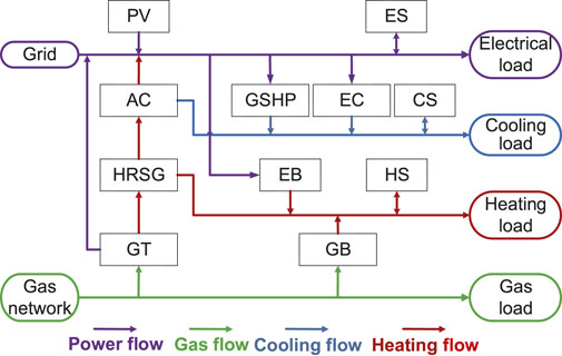
FIGURE 1. IES structure and energy flow.

2.2 Constructing an IES model

2.2.1 The part CCHP

The part CCHP model is built as follows:

$\left\{\begin{array}{c}\hfill P_{\mathrm{g}\mathrm{t}}\left(t\right)=G_{\mathrm{g}\mathrm{t}}\left(t\right)K_{\text{g}}{\eta }_{\mathrm{g}\mathrm{t}}\hfill \\ \hfill H_{\mathrm{h}\mathrm{g}}\left(t\right)=\frac{P_{\mathrm{g}\mathrm{t}}\left(t\right)}{{\eta }_{\mathrm{g}\mathrm{t}}}{\eta }_{\mathrm{h}\mathrm{g}}\hfill \\ \hfill C_{\mathrm{a}\mathrm{c}}\left(t\right)=H_{\mathrm{h}\mathrm{g}}\left(t\right){\eta }_{\mathrm{a}\mathrm{c}}\hfill \end{array}\right.(1)$

where P_gt, H_hg, and C_ac are the output electric power, thermal power, and cold power, respectively; G_gt is the natural gas consumption; K_g is the gas–heat conversion factor; η_gt is the power generation efficiency; η_hg is the heat generation efficiency; and η_ac is the heat and cold conversion efficiency.

2.2.2 The part EC

The part EC is expressed as follows:

$C_{\mathrm{e}\mathrm{c}}\left(t\right)=P_{\mathrm{e}\mathrm{c}}\left(t\right){\eta }_{\mathrm{e}\mathrm{c}},(2)$

where C_ec is the cooling power; P_ec is the input electrical power; and η_ec is the cooling efficiency.

2.2.3 The part GB

The part GB is shown as follows:

$H_{\mathrm{g}\mathrm{b}}=G_{\mathrm{g}\mathrm{b}}{K}_{\text{g}}{\eta }_{\mathrm{g}\mathrm{b}},(3)$

where H_gb is the heat production power; G_gb is the natural gas consumption; and η_gb is the gas-to-heat conversion efficiency.

2.2.4 The part EB

The part EB is expressed as follows:

$H_{\mathrm{e}\mathrm{b}}\left(t\right)=P_{\mathrm{e}\mathrm{b}}\left(t\right){\eta }_{\mathrm{e}\mathrm{b}},(4)$

where H_eb is the heating power; P_eb is the input electric power; and η_eb is the heating efficiency.

2.2.5 The part GSHP

The part GSHP is expressed as follows:

$C_{\mathrm{g}\mathrm{p}}\left(t\right)=P_{\mathrm{g}\mathrm{p}}\left(t\right){\eta }_{\mathrm{g}\mathrm{p}},(5)$

where C_gp is the cooling power; P_gp is the input electrical power; and η_gp is the cooling efficiency.

2.2.6 The part energy storage systems

Electric energy storage, CS, and HS share a similar working principle and energy conversion relationship; here, these are expressed in a unified energy storage model, and the power model of energy storage devices is as follows (Asl et al., 2022):

$E^s\left(t\right)=E^s\left(t-1\right)\left(1-{\eta }_{\mathrm{l}\mathrm{o}\mathrm{s}\mathrm{s}}^s\right)+{\eta }_{\mathrm{c}\mathrm{h}\mathrm{a}\mathrm{r}}^s{P}_{\mathrm{c}\mathrm{h}\mathrm{a}\mathrm{r}}^s\left(t\right)-\frac{P_{\mathrm{d}\mathrm{i}\mathrm{s}}^s\left(t\right)}{{\eta }_{\mathrm{d}\mathrm{i}\mathrm{s}}^s},(6)$

where E^s(t) is the storage capacity of the energy storage device at time t; $P_{\mathrm{c}\mathrm{h}\mathrm{a}\mathrm{r}}^s(t)$ and $P_{\mathrm{d}\mathrm{i}\mathrm{s}}^s(t)$ are the storage charging and discharging power of the energy storage device at time t, respectively; ${\eta }_{\mathrm{l}\mathrm{o}\mathrm{s}\mathrm{s}}^s$, ${\eta }_{\mathrm{c}\mathrm{h}\mathrm{a}\mathrm{r}}^s$, and η^s_dis are the self-loss rate, charging efficiency, and discharging efficiency of the energy storage device, respectively; and s = 1, 2, 3 are the electric energy storage, CS, and HS, respectively.

$\left\{\begin{array}{c}\hfill E_{\min }^s\le E^s\left(t\right)\le E_{\max }^s\hfill \\ \hfill 0\le P_{\mathrm{c}\mathrm{h}\mathrm{a}\mathrm{r}}^s\left(t\right)\le {\alpha }_{\mathrm{c}\mathrm{h}\mathrm{a}\mathrm{r}}^s\left(t\right)P_{\mathrm{c}\mathrm{h}\mathrm{a}\mathrm{r},\mathrm{m}\mathrm{a}\mathrm{x}}^s\hfill \\ \hfill 0\le P_{\mathrm{d}\mathrm{i}\mathrm{s}}^s\left(t\right)\le {\alpha }_{\mathrm{d}\mathrm{i}\mathrm{s}}^s\left(t\right)P_{\mathrm{d}\mathrm{i}\mathrm{s},\mathrm{m}\mathrm{a}\mathrm{x}}^s\hfill \\ \hfill {\alpha }_{\mathrm{c}\mathrm{h}\mathrm{a}\mathrm{r}}^s\left(t\right)+{\alpha }_{\mathrm{d}\mathrm{i}\mathrm{s}}^s\left(t\right)\le 1\hfill \\ \hfill E_1^s\left(t\right)=E{\left(t\right)}_{24}^s\hfill \end{array}\right.(7)$

where $E_{\max }^s$ and $E_{\min }^s$ are the upper and lower limits of the energy storage capacity of the energy storage device, respectively; $P_{\mathrm{c}\mathrm{h}\mathrm{a}\mathrm{r},\mathrm{m}\mathrm{a}\mathrm{x}}^{s}and{P}_{\mathrm{d}\mathrm{i}\mathrm{s},\mathrm{m}\mathrm{a}\mathrm{x}}^s$ are the maximum charging and discharging power of the energy storage device, respectively; ${\alpha }_{\mathrm{c}\mathrm{h}\mathrm{a}\mathrm{r}}^s(t)$ and ${\alpha }_{\mathrm{d}\mathrm{i}\mathrm{s}}^s(t)$ are the states of charging and discharging, respectively; and 1 means the device is in a charging or discharging state and 0 means the device stops charging and is in a discharging state.

3 Electricity–gas–cooling load demand response model

The demand response approach utilized in this work comprises a price-based electricity–gas load demand response and an adjustable cooling load demand response.

3.1 Electricity–gas load demand response

This paper considers price-based electricity–gas load demand response, and a price-based demand response model based on the load price elasticity coefficient matrix is developed to guide customers in responding to changes in energy prices in order to adjust load demand. The change in load is represented by a price elasticity matrix based on the price elasticity coefficient while employing time-sharing electricity and gas pricing (Tan et al., 2020). The elasticity coefficient is defined as the ratio of the rate of change in load demand to the rate of change in price and is calculated as follows:

${\epsilon }_{ij}^x=\frac{\mathrm{\Delta }{Q}_j^x}{Q_j^x}/\frac{\mathrm{\Delta }{P}_i^x}{P_i^x},(8)$

where ${\epsilon }_{ij}^x$ is the price elasticity coefficient; $Q_j^x$ and $\mathrm{\Delta }{Q}_j^x$ are the load demand and load change, respectively; ${\epsilon }_{ij}^x$ is the self-elasticity coefficient when i = j; ${\epsilon }_{ij}^x$ is the cross-elasticity coefficient when i ≠ j; and x = 1 for electric load and x = 2 for gas load. The load change reflected by the price elasticity matrix can be calculated using the price elasticity coefficient:

$\left[\begin{array}{c}\hfill \mathrm{\Delta }{Q}_1^x/Q_1^x\hfill \\ \hfill \mathrm{\Delta }{Q}_2^x/Q_2^x\hfill \\ \hfill ⋮\hfill \\ \hfill \mathrm{\Delta }{Q}_n^x/Q_n^x\hfill \end{array}\right]=\left[\begin{array}{cccc}\hfill {\epsilon }_{11}^x\hfill & \hfill {\epsilon }_{12}^x\hfill & \hfill \cdots \hfill & \hfill {\epsilon }_{1n}^x\hfill \\ \hfill {\epsilon }_{21}^x\hfill & \hfill {\epsilon }_{22}^x\hfill & \hfill \cdots \hfill & \hfill {\epsilon }_{2n}^x\hfill \\ \hfill ⋮\hfill & \hfill ⋮\hfill & \hfill \hfill & \hfill ⋮\hfill \\ \hfill {\epsilon }_{n1}^x\hfill & \hfill {\epsilon }_{n2}^x\hfill & \hfill \cdots \hfill & \hfill {\epsilon }_{nn}^x\hfill \end{array}\right]\left[\begin{array}{c}\hfill \mathrm{\Delta }{P}_1^x/P_1^x\hfill \\ \hfill \mathrm{\Delta }{P}_2^x/P_2^x\hfill \\ \hfill ⋮\hfill \\ \hfill \mathrm{\Delta }{P}_n^x/P_n^x\hfill \end{array}\right].(9)$

In order to find the price elasticity matrix consisting of the price elasticity coefficients in Equation 9, assuming that for a given time interval l, the energy price at any moment i has the same effect on the consumption of the same type of energy at moments i + l, the following assumptions are made in this paper:

$\begin{array}{ll}\hfill {\epsilon }_{11}^x& ={\epsilon }_{22}^x=\cdots ={\epsilon }_{nn}^x={\epsilon }_0\hfill \\ {\epsilon }_{12}^x\hfill & ={\epsilon }_{23}^x=\cdots ={\epsilon }_{\left(n-1\right)n}^x={\epsilon }_1^x\hfill \\ {\epsilon }_{13}^x\hfill & ={\epsilon }_{24}^x=\cdots ={\epsilon }_{\left(n-2\right)n}^x={\epsilon }_2^x\hfill \\ {\epsilon }_{21}^x\hfill & ={\epsilon }_{32}^x=\cdots ={\epsilon }_{n\left(n-1\right)}^x={\epsilon }_{-1}^x\hfill \\ {\epsilon }_{31}^x\hfill & ={\epsilon }_{12}^x=\cdots ={\epsilon }_{n\left(n-2\right)}^x={\epsilon }_{-2}^x\hfill \\ \hfill & \cdots \hfill \end{array}.(10)$

Therefore, Equation 9 can be simplified as follows:

$\frac{\mathrm{\Delta }{Q}_i^x}{Q_i^x}=\sum _{l=-m}^{+m}{\epsilon }_l\frac{\mathrm{\Delta }{P}_{i+l}^x}{P_{i+l}^x},(11)$

where i = 1, 2, …, n and $P_{i+l}^x$ are the energy prices at neighboring moment i at a distance l; ε_l is the response elasticity coefficient; and m is the range of moments that have an effect on energy prices at moment i. The specific procedure for finding the price elasticity matrix is as follows:

Step 1. Based on the historical energy use data of the studied IES (June–July 2022), corresponding to time period i, the average value of energy prices p_i and the average value of energy use q_i are calculated as follows:

$p_i=\frac{R_{fi}+R_{gi}+R_{pi}}{q_{fi}+q_{gi}+q_{pi}},(12)$

$q_i^x=q_{fi}^x+q_{gi}^x+q_{pi}^x,(13)$

where R is the energy price; q is the energy usage; and the subscripts f, g, and p are the peak, valley, and normal periods, respectively.

Step 2. Outlier handling

The 3σ criterion is chosen to remove outliers from the sample.

$|v_k|=X_k-\bar{X}>3\sigma .(14)$

If the residual satisfies Equation 14, the value is considered an outlier. Since the standard deviation σ is usually unknown, the experimental standard deviation difference s (X_k) is used instead of σ. The formula for s (X_k) is as follows:

$s\left(X_k\right)=\sqrt{\frac{1}{n-1}\left[\sum _{k=1}^n{\left(X_k-\bar{X}\right)}^2\right]},(15)$

where X_k is the value of the first k samples; $\bar{X}$ is the mean value of the samples.

Step 3. The rate of change of energy and energy prices is calculated. The rate of change of energy and energy prices in Equation 9 is calculated using Equations 15, 16, respectively:

$\frac{\mathrm{\Delta }{Q}_i^x}{Q_i^x}=\frac{Q_{i2}^x-Q_{i1}^x}{Q_{i1}^x},(16)$

$\frac{\mathrm{\Delta }{P}_i^x}{P_i^x}=\frac{P_{i2}^x-P_{i1}^x}{P_{i1}^x},(17)$

where $P_{i2}^x$ is the average value of energy price in July at i period; $P_{i1}^x$ is the average value of energy price in June at i period; $Q_{i2}^x$ is the energy usage in July at i period; and $Q_{i1}^x$ is the energy usage in June at i period.

Step 4. The price elasticity coefficient matrix based on Equation 11 is calculated. A multiple regression algorithm is applied to calculate the price elasticity coefficient ɛ_l, l = −m, − m + 1, …, + m.

After using the time-sharing electricity–gas price, the following formula may be derived based on Equation 9:

$\begin{array}{ll}\hfill \left[\begin{array}{c}\hfill Q_1^{*x}\hfill \\ \hfill Q_2^{*x}\hfill \\ \hfill ⋮\hfill \\ \hfill Q_n^{*x}\hfill \end{array}\right]& =\left[\begin{array}{c}\hfill Q_1^x\hfill \\ \hfill Q_2^x\hfill \\ \hfill ⋮\hfill \\ \hfill Q_n^x\hfill \end{array}\right]+\left[\begin{array}{cccc}\hfill Q_1^x\hfill & \hfill 0\hfill & \hfill \cdots \hfill & \hfill 0\hfill \\ \hfill 0\hfill & \hfill Q_2^x\hfill & \hfill \cdots \hfill & \hfill 0\hfill \\ \hfill ⋮\hfill & \hfill ⋮\hfill & \hfill \hfill & \hfill ⋮\hfill \\ \hfill 0\hfill & \hfill 0\hfill & \hfill \cdots \hfill & \hfill Q_n^x\hfill \end{array}\right]\left[\begin{array}{c}\hfill \mathrm{\Delta }{Q}_1^x/Q_1^x\hfill \\ \hfill \mathrm{\Delta }{Q}_2^x/Q_2^x\hfill \\ \hfill ⋮\hfill \\ \hfill \mathrm{\Delta }{Q}_n^x/Q_n^x\hfill \end{array}\right],\hfill \end{array}(18)$

where $Q_n^{*x}$ is the electricity–gas load demand after the introduction of time-of-use pricing.

3.2 Cooling load demand response

Adjustable cooling load demand response modifies the cooling load within the user’s temperature comfort range based on the ambiguity of the user’s temperature demand and transforms the cooling load curve into a cooling load interval, increasing system scheduling flexibility. A building heat balance model is a physical description of the building heat exchange process that can analyze the principle and process of temperature change in the building, describe the process of heat gain and loss in the building, and obtain the connection between temperature and cooling power in the building (Triolo et al., 2023). The following heat balance equation can be used to describe the temperature change inside the building:

$\left(c_{\mathrm{g}\mathrm{a}\mathrm{s}}{m}_{\mathrm{g}\mathrm{a}\mathrm{s}}+c_{\text{s}}{m}_{\text{s}}\right)\frac{\mathrm{d}{T}_{\text{b}}}{\mathrm{d}t}=q_{\mathrm{l}\mathrm{o}\mathrm{a}\mathrm{d}}\left(t\right)-q_{\text{c}}\left(t\right),(19)$

where c_gas and c_s are the specific heat capacity of air and the specific heat capacity of the envelope, respectively; m_gas and m_s are the air mass and the envelope mass, respectively; dT_b/dt is the differentiation of room temperature with respect to time; q_c(t) is the cooling power; and q_load(t) is the building load.

The building load q_load(t) consists of the following components:

$q_{\mathrm{l}\mathrm{o}\mathrm{a}\mathrm{d}}\left(t\right)=q_1\left(t\right)+q_2\left(t\right)+q_3\left(t\right),(20)$

where q₁(t) is the heat exchange between the maintenance structure and the environment; q₂(t) is the heat transfer from the outside air; and q₃(t) is the heat dissipation inside the building. q₁(t), q₂(t), and q₃(t), respectively, can be expressed as

$\left\{\begin{array}{c}{q}_1\left(t\right)=KF\left(T_{\mathrm{i}\mathrm{n}}\left(t\right)-T_{\mathrm{o}\mathrm{u}\mathrm{t}}\left(t\right)\right)\hfill \\ q_2\left(t\right)=\left(T_{\mathrm{i}\mathrm{n}}\left(t\right)-T_{\mathrm{o}\mathrm{u}\mathrm{t}}\left(t\right)\right)c_{\mathrm{g}\mathrm{a}\mathrm{s}}{\rho }_{\mathrm{g}\mathrm{a}\mathrm{s}}V\hfill \\ q_3\left(t\right)=A\left(e\left(t\right)+p_{\text{e}}\left(t\right)\right)\hfill \end{array}\right.(21)$

where K is the average heat transfer coefficient of the maintenance structure; F is the heat transfer area of the maintenance structure; T_in(t) is the indoor temperature; T_out(t) is the outdoor temperature; ρ_gas is the air density; V is the air exchange volume; A is the floor area; e(t) is the amount of heat dissipated by the equipment per unit area; and P_e(t) is the heat dissipation power per unit area. The discrete treatment of the building heat balance equation is as follows:

$q_{\text{c}}\left(t\right)=-\left\{\frac{\left(T_{\mathrm{i}\mathrm{n}}\left(t+1\right)-T_{\mathrm{i}\mathrm{n}}\left(t\right)\right)\left(c_{\mathrm{g}\mathrm{a}\mathrm{s}}{m}_{\mathrm{g}\mathrm{a}\mathrm{s}}+c_{\text{s}}{m}_{\text{s}}\right)}{\mathrm{\Delta }t}+q_{\mathrm{l}\mathrm{o}\mathrm{a}\mathrm{d}}\left(t\right)\right\}.(22)$

According to the aforementioned calculation, the user’s cooling load demand is proportional to the indoor temperature and equals the cooling power under supply–demand balance. Thus, the adjustment interval of the cold power supplied by the IES may be estimated based on the user’s temperature comfort range, reducing the burden of delivering energy during the peak cooling period.

4 Multi-objective optimal scheduling for the IES

The multi-objective optimal function is constructed as follows:

$F=\min \left\{F_1,F_2,F_3\right\},(23)$

where F₁ is the system operating cost; F₂ is the system carbon emission; and F₃ is the inverse of the system exergy efficiency.

4.1 Economical goal

The daily operating cost of the system includes the purchase cost of electricity and gas f_buy and the operation and maintenance cost of each equipment f_om.

$F_1=f_{\mathrm{b}\mathrm{u}\mathrm{y}}+f_{\mathrm{o}\mathrm{m}},(24)$

$f_{\mathrm{b}\mathrm{u}\mathrm{y}}=\sum _{t=1}^{24}{P}_{\mathrm{g}\mathrm{r}\mathrm{i}\mathrm{d}}\left(t\right)C_{\mathrm{g}\mathrm{r}\mathrm{i}\mathrm{d}}\left(t\right)+\sum _{t=1}^{24}{G}_{\mathrm{g}\mathrm{r}\mathrm{i}\mathrm{d}}\left(t\right)C_{\mathrm{g}\mathrm{a}\mathrm{s}}\left(t\right),(25)$

where P_grid(t) is the purchased power at time t, C_grid(t) is the price of electricity at time t, G_grid(t) is the purchased gas volume at time t, and C_gas(t) is the price of gas at time t.

$f_{\mathrm{o}\mathrm{m}}=\sum _{i=1}^n\sum _{t=1}^{24}{P}_i\left(t\right){\eta }_i,(26)$

where P_i(t) is the power output of the ith device at time t; η_i is the operation and maintenance cost of the ith equipment output.

4.2 Environmental goal

Carbon emissions from power and gas purchases are included in the IES carbon emissions. The entire system’s carbon emissions are calculated using the unit carbon emission factor as follows:

$F_2=\sum _{t=1}^{24}{P}_{\mathrm{g}\mathrm{r}\mathrm{i}\mathrm{d}}\left(t\right){\lambda }_{\mathrm{g}\mathrm{r}\mathrm{i}\mathrm{d}}\left(t\right)+\sum _{t=1}^{24}{G}_{\mathrm{g}\mathrm{r}\mathrm{i}\mathrm{d}}\left(t\right){\lambda }_{\mathrm{g}\mathrm{a}\mathrm{s}},(27)$

where λ_grid is the purchased power carbon emission factor; λ_gas is the purchased gas carbon emission factor.

4.3 Exergy target

The IES contains several types of energy with varying characteristics. Exergy can represent the “quantity” as well as the “quality” of energy. We introduce an energy quality system to measure the losses in each energy source’s conversion process and determine the utilization of each energy source, i.e., exergy efficiency (Chen et al., 2022). The inverse of exergy efficiency is used as the optimization objective in the following equation:

$F_3=\frac{\sum _{t=1}^{\mathrm{24}}\left(P_{\mathrm{l}\mathrm{d}}\left(t\right){\lambda }_{\text{e}}+H_{\mathrm{l}\mathrm{d}}\left(t\right){\lambda }_{\text{h}}+C_{\mathrm{l}\mathrm{d}}\left(t\right){\lambda }_{\text{c}}+G_{\mathrm{l}\mathrm{d}}\left(t\right){\lambda }_{\text{g}}\right)}{\sum _{t=1}^{\mathrm{24}}\left(P_{\mathrm{g}\mathrm{r}\mathrm{i}\mathrm{d}}\left(t\right){\lambda }_{\text{e}}+P_{\mathrm{p}\mathrm{v}}\left(t\right){\lambda }_{\mathrm{p}\mathrm{v}}+G_{\mathrm{g}\mathrm{r}\mathrm{i}\mathrm{d}}\left(t\right){\lambda }_{\text{g}}\right)},(28)$

where P_ld(t), H_ld(t), C_ld(t), and G_ld(t) are the electrical, thermal, cooling, and gas loads of the system at time t, respectively; λ_e, λ_h, λ_c, λ_g, and λ_pv are the energy quality coefficients of electrical, thermal, cooling, and PV, respectively; and P_pv(t) is the PV power generated at time t.

4.4 Constraints and conditions

The IES is subjected to power balance constraints and conditions when solving optimal scheduling. The electrical power balance constraint is shown as follows:

$\begin{array}{ll}\hfill P_{\mathrm{g}\mathrm{t}}\left(t\right)+P_{\mathrm{p}\mathrm{v}}\left(t\right)+P_{\mathrm{d}\mathrm{i}\mathrm{s}}^1\left(t\right)+P_{\mathrm{g}\mathrm{r}\mathrm{i}\mathrm{d}}\left(t\right)& =P_{\mathrm{e}\mathrm{c}}\left(t\right)+P_{\mathrm{e}\mathrm{b}}\left(t\right)+P_{\mathrm{g}\mathrm{p}}\left(t\right)\hfill \\ \hfill & +P_{\mathrm{l}\mathrm{d}}\left(t\right)+P_{\mathrm{c}\mathrm{h}\mathrm{a}\mathrm{r}}^1\left(t\right).\hfill \end{array}(29)$

The thermal power balance constraint is

$H_{\mathrm{g}\mathrm{b}}\left(t\right)+H_{\mathrm{e}\mathrm{b}}\left(t\right)+H_{\mathrm{h}\mathrm{g}}\left(t\right)+P_{\mathrm{d}\mathrm{i}\mathrm{s}}^3\left(t\right)=H_{\mathrm{l}\mathrm{d}}\left(t\right)+P_{\mathrm{c}\mathrm{h}\mathrm{a}\mathrm{r}}^3\left(t\right).(30)$

The cooling power balance constraint is

$C_{\mathrm{a}\mathrm{c}}\left(t\right)+C_{\mathrm{e}\mathrm{c}}\left(t\right)+C_{\mathrm{g}\mathrm{p}}\left(t\right)+P_{\mathrm{d}\mathrm{i}\mathrm{s}}^2\left(t\right)=C_{\mathrm{l}\mathrm{d}}\left(t\right)+P_{\mathrm{c}\mathrm{h}\mathrm{a}\mathrm{r}}^2\left(t\right).(31)$

The gas power balance constraint is

$G_{\mathrm{g}\mathrm{r}\mathrm{i}\mathrm{d}}\left(t\right)=G_{\mathrm{g}\mathrm{t}}\left(t\right)+G_{\mathrm{g}\mathrm{b}}+G_{\mathrm{l}\mathrm{d}}\left(t\right).(32)$

The system power and gas purchase constraints are

$\left\{\begin{array}{c}\hfill 0\le G_{\mathrm{g}\mathrm{r}\mathrm{i}\mathrm{d}}\left(t\right)\le G_{\mathrm{b}\mathrm{u}\mathrm{y}\mathrm{m}\mathrm{a}\mathrm{x}}\hfill \\ \hfill 0\le P_{\mathrm{g}\mathrm{r}\mathrm{i}\mathrm{d}}\left(t\right)\le P_{\mathrm{g}\mathrm{r}\mathrm{i}\mathrm{d}\mathrm{m}\mathrm{a}\mathrm{x}}\hfill \end{array}\right.(33)$

where G_buymax is the upper limit of purchased gas power; P_gridmax is the upper limit of purchased electricity power.

According to the “Office Building Design Standards” in China, the indoor temperature of office buildings in summer should be in the range of 25°C–28°C. The temperature comfort constraint is

$25\le T\left(t\right)\le 28.(34)$

4.5 Model solving

In this paper, NSGA-II based on Tent mapping chaos optimization is used to solve the proposed multi-objective optimization model, due to its advantages of large search space and fast convergence (Verma et al., 2021). The specific solving process is depicted in Figure 2. After obtaining the Pareto optimal frontier solution set using NSGA-II based on Tent mapping chaos optimization, the optimal scheduling scheme is selected using the VIKOR decision method, and the specific process is as follows (Zheng and Wang, 2020):

FIGURE 2

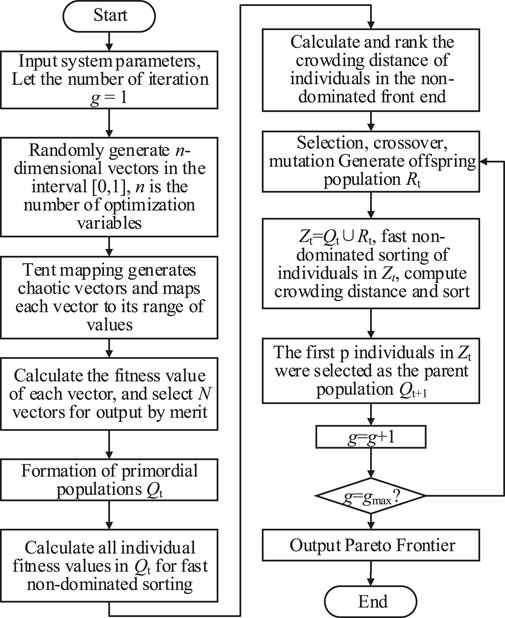
FIGURE 2. NSGA-II based on Tent mapping chaos optimization.

Step 1. Let A = {A₁, A₂, …, A_n} be the set of force solutions to be selected, n = 100; G = {G₁, G₂, …, G_m} be the set of objectives, m = 3; and W = {w₁, w₂, …, w_m} be the set of objective weights.

Step 2. The raw data x_ij = {i = 1, 2, …, n; j = 1, 2, ⋯m} are normalized.

$v_{ij}=\frac{x_{ij}}{\sqrt{\sum _{i=1}^n{x}_{ij}^2}},(35)$

where v_ij is the normative value of the j objective of the i scenario.

Step 3. The positive and negative ideal solutions are obtained.

$\left\{\begin{array}{c}\hfill r^{+}=\left\{\max x_{i1},\max x_{i2},\dots ,\max x_{im}\right\},\hfill \\ \hfill r^{-}=\left\{\min x_{i1},\min x_{i2},\dots ,\min x_{im}\right\}\hfill \end{array}\right.(36)$

where r⁺ and r⁻ are the positive and negative ideal solutions, respectively.

Step 4. The group benefit values and individual regret values are calculated.

$S_i=\sum w_{ij}\left(\frac{r_j^{+}-v_{ij}}{r_j^{+}-r_j^{-}}\right),(37)$

$R_i=\max \left\{\left.w_{ij}\left(\frac{r_j^{+}-v_{ij}}{r_j^{+}-r_j^{-}}\right)\right\}\right.(38)$

where S_i and R_i are the group effect value and individual regret value of the i decision option, respectively.

Step 5. The decision index value Q_i based on S_i, R_i is calculated.

$Q_i=v\frac{S_i-S^{-}}{S^{+}-S^{-}}+\left(1-v\right)\frac{R_i-R^{-}}{R^{+}-R^{-}},(39)$

where Q_i is the value of the decision indicator; S⁺ and S⁻ are the maximum and minimum values of group effect, respectively; and R⁺ and R⁻ are the maximum and minimum values of individual regret, respectively.

Step 6. According to the decision index values of each solution, the solution corresponding to the first ranked index value is the optimal solution.

5 Example analysis

5.1 Parameter settings

The Sino-German Ecological Park in Qingdao, China, is chosen as the research object to investigate the applicability and effectiveness of the proposed IES multi-objective optimal dispatch model incorporating exergy efficiency and demand responsiveness (DR). The multi-objective optimal scheduling analysis is performed in this example based on the electricity, gas, cooling, and heating loads in typical summer days. The global scheduling time is 24 h, and the unit scheduling time is 1 h. Figure 3 depicts the system’s projection for power, gas, cooling, and heating loads and solar output. The price information of natural gas and electricity used in this case study is listed in Table 1. Table 2 lists the economic parameters of the equipment. Table 3 lists the parameters of the modeling. Among them, IES internal equipment parameters, energy storage equipment parameters, and energy time-of-use prices are derived from Wang et al. (2022). The following NSGA-II settings are considered: the population size is 50, the maximum number of iterations is 300, the crossover percentage is 0.7, and the mutation percentage is 0.3. The average summer days of IES are chosen for this paper’s energy supply study. Because the heat load is small and stable, it is excluded in demand response.

FIGURE 3

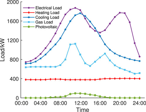
FIGURE 3. Electrical, gas, cooling, and heating loads and PV output forecast.

TABLE 1

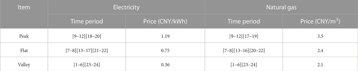
TABLE 1. Prices of natural gas and electricity.

TABLE 2

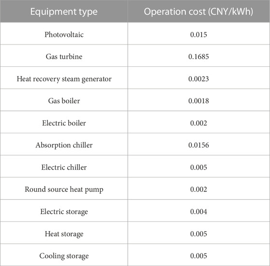
TABLE 2. Economic parameters of equipment.

TABLE 3

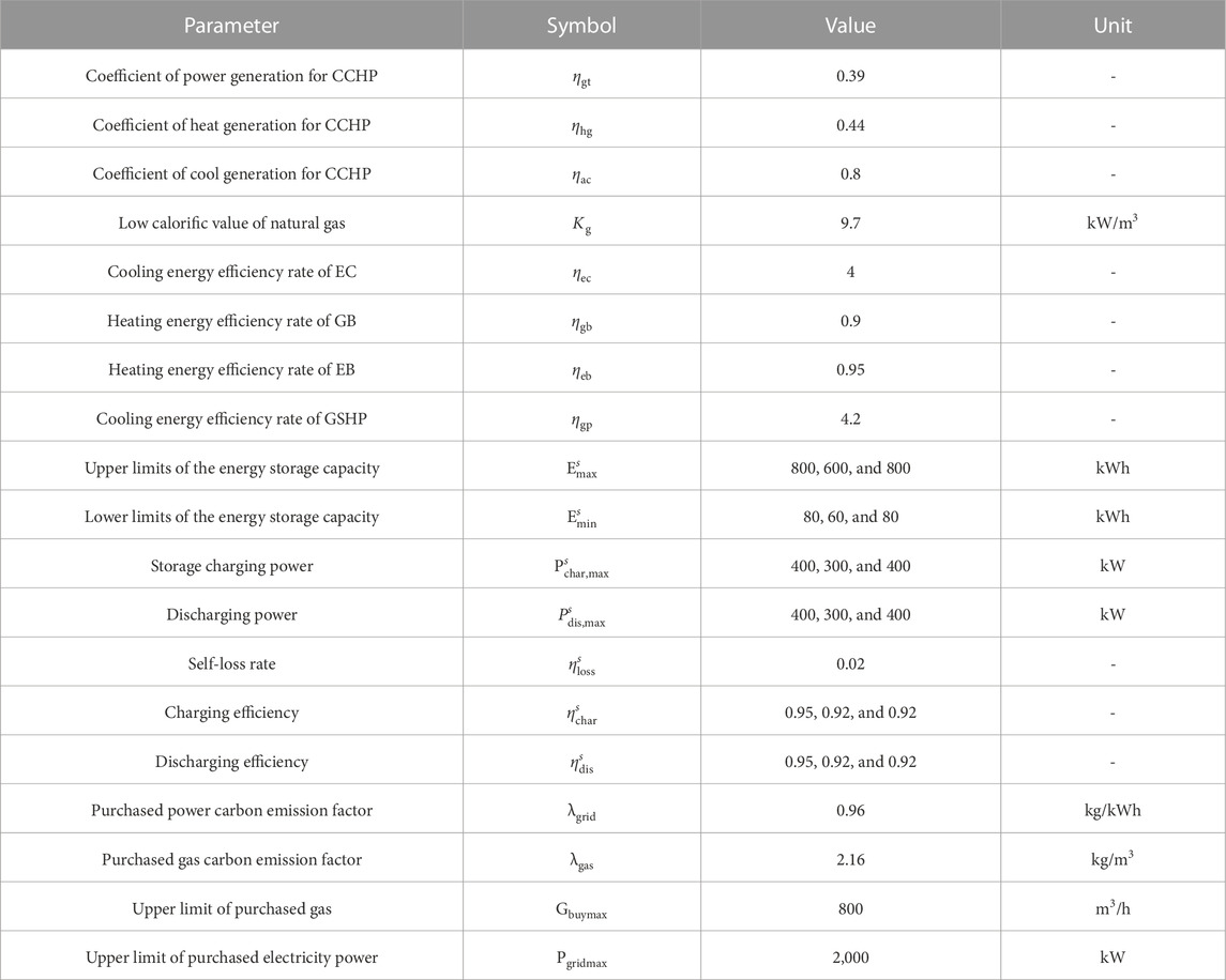
TABLE 3. Parameters of the modeling.

5.2 Analysis of the results

To validate the feasibility and effectiveness of the IES optimal scheduling model developed in this paper, five scenarios are set up for comparative analysis, and the settings for each scenario are shown in Table 4. The optimization outcomes under each scenario are solved after optimization computation, and the system operation cost, carbon emission, and energy efficiency are compared, and the optimum scheduling results are shown in Table 5. As shown in Table 5, the performance of individual indexes in Scenario 4 is slightly worse than that in Scenarios 1, 2, and 3; however, it can take into account the three indices of system economy, environmental protection, and energy efficiency at the same time. Compared to Scenario 1, exergy efficiency improves by 5.1%; compared to Scenario 2, carbon emissions are decreased by 3.5%; and compared to Scenario 3, operation costs are lowered by 5.2%. As a result, the model suggested in this study can meet IES scheduling criteria for numerous purposes, such as economy, environmental protection, and exergy efficiency.

TABLE 4

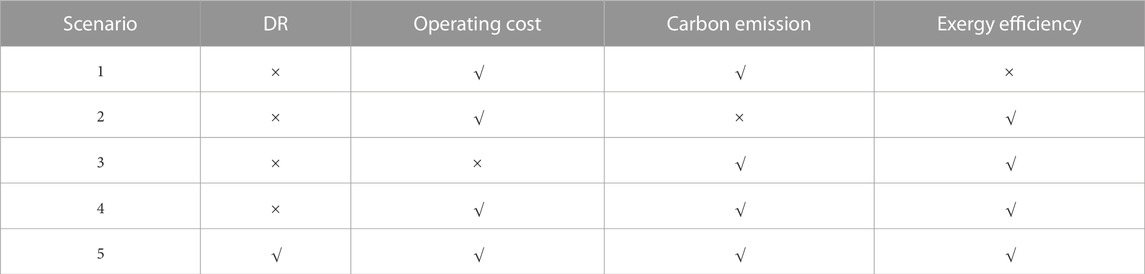
TABLE 4. Various scenario settings.

TABLE 5

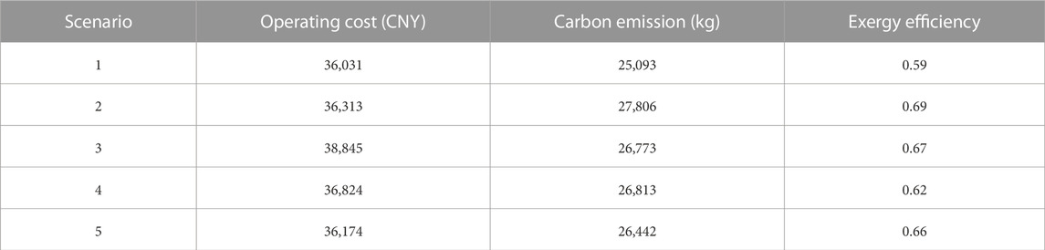
TABLE 5. System operating costs, carbon emissions, and exergy efficiency for each scenario.

The load variations following demand response are depicted in Figure 4 and Figure 5. When combined with Table 5, it can be observed that all indicators of Scenario 5 are better than those of Scenario 4, in which energy efficiency is increased by 6.4%, carbon emissions are decreased by 1.3%, and operation costs are lowered by 1.7%. This is primarily due to the fact that after demand response, IES can appropriately cut the peak values of electric load, gas load, and cooling load while satisfying the basic load demand and maintaining a comfortable temperature and, lowering the cost of purchasing high-priced energy during the peak period; at the same time, it can shift the peak load, allowing for multi-objective optimization to reduce carbon emissions and improve exergy efficiency.

FIGURE 4

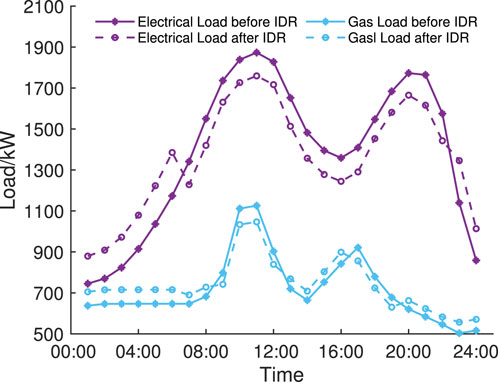
FIGURE 4. Electricity load and gas load before and after the introduction of demand responsiveness.

FIGURE 5

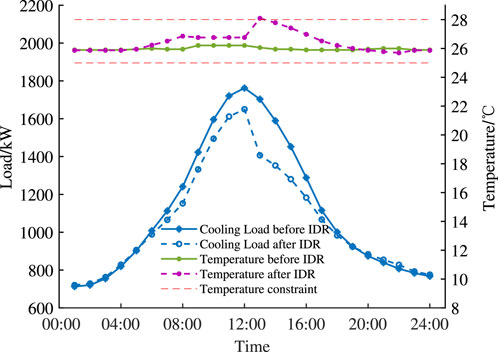
FIGURE 5. Comparison of cooling load and temperature before and after the introduction of demand responsiveness.

The peak–valley difference of electric load after demand response decreases by 21.9% and the peak–valley difference of gas load after demand response decreases by 17.8% compared to those before demand response. The load fluctuation is leveled off, which is due to the impact of price response on users’ energy consumption habits, and users’ loads are shifted downward and upward during peak and valley hours, respectively, as shown in Figure 4 and Figure 5. The efficiency of price-based demand response for optimizing electricity–gas load is demonstrated. During the peak cold load period, the cold load is properly reduced to ensure the user’s comfort, relieving supply pressure during the peak energy consumption period. This is due to the human body’s ambiguity for temperature changes within a certain range, and adjusting the cold load to change the temperature within this range has no effect on the comfortable temperature, so the cold load curve is transformed into a cold load interval, transforming the cold load into a flexible adjustable load to participate in demand response to enhance system scheduling flexibility. The electric, gas, and cooling load curves can be efficiently smoothed using demand response, ensuring improved system operating economy, environmental protection, and exergy efficiency.

The Pareto solution set of Scenario 5 is illustrated in Figure 6, demonstrating that the low operating cost, low carbon emission, and high exergy efficiency of IES are three competing optimization objectives, and obtaining the optimal solution simultaneously is difficult. As a result, the model developed in this paper can satisfy IES’s optimal scheduling requirements in terms of economy, environmental protection, and exergy efficiency. Decision-makers in the multi-objective optimal decision method used in this study can alter the VIKOR decision weight parameters based on the real needs of the project to acquire the appropriate optimal scheduling solution.

FIGURE 6

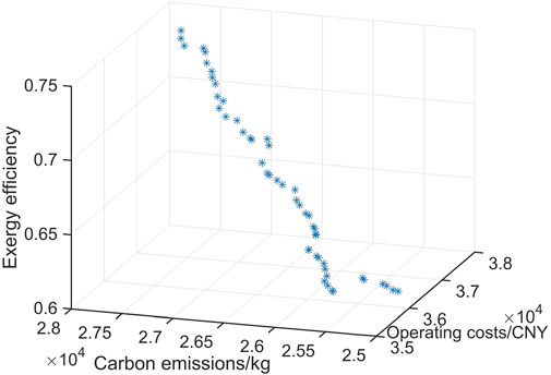
FIGURE 6. Diagram of electrical power balance.

The optimal dispatching result of Scenario 5 is shown in Figure 7, Figure 8, Figure 9, and Figure 10. Due to the cost-effectiveness, minimal carbon footprint, and high exergy efficiency of PV, it is completely consumed during the dispatching procedure. During 23:00–06:00, the system purchases low-cost electricity from the grid as its primary supply and from GT as its supplementary supply, while the storage apparatus stores electricity. At this time, the cold load is low, with EC and GSHP as the primary supply method and AC as the supplementary supply; during 07:00–10:00, the electric load and cold load continue to increase, the price of electricity is moderate, and the joint power supply equipment can meet the needs of a variety of loads; during 11:00–13:00, the electric load and cold load reach their peak, the price of electricity is at its highest, and GT generation is more advantageous. AC as the main refrigeration equipment, which can use low-grade thermal energy to cool, has a more balanced exergy efficiency and economy compared to the consumption of high-grade electrical energy to cool the electric refrigeration equipment; during 14:00–17:00, the cold load demand is greater, the electricity price is flat, and the system is suited to increase the output of the electric refrigeration equipment; and during 18:00–22:00, which are the peak electricity price hours, the output of the electric refrigeration equipment should be decreased.

FIGURE 7

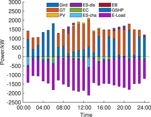
FIGURE 7. Results of electrical power balance.

FIGURE 8

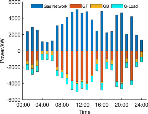
FIGURE 8. Results of gas power balance.

FIGURE 9

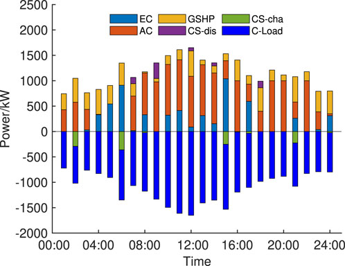
FIGURE 9. Results of cooling power balance.

FIGURE 10

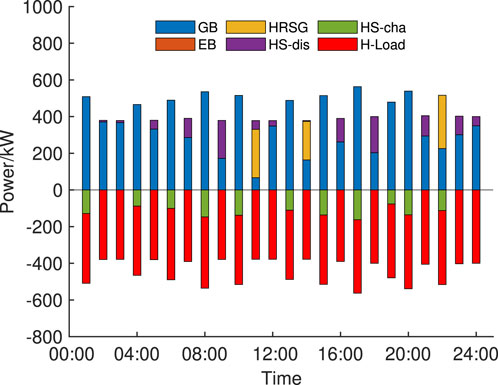
FIGURE 10. Results of heating power balance.

6 Discussion and limitations

This section will provide a broader analysis of the multi-objective optimal scheduling model proposed in this paper, discussing its strengths and limitations. In addition to considering the modeling and technological diversity of information exchange, the model’s impact on the intensity of information exchange among the participants of an IES will be explored.

6.1 Advantages of the model

Multi-objective optimization: The model proposed in this paper effectively balances multiple objectives, including system operating costs, carbon emissions, and exergy. By providing a Pareto optimal frontier solution set, it enables decision-makers to weigh the trade-offs and make informed choices that are in line with their priorities. In this paper, we use NSGA-II to achieve efficient solution space exploration and obtain diverse sets of Pareto optimal solutions. This feature enables decision-makers to identify a range of feasible and desirable solutions. Integrated demand response: The introduction of a demand response mechanism allows dynamic load regulation, promotes demand-side management and energy conservation, and helps improve the overall economic and environmental performance of the IES. The model takes into account user’s comfort when optimizing energy scheduling, ensuring user’s comfort, enhancing user’s satisfaction, and increasing user’s participation in demand response programs.

6.2 Limitations of the model

Scalability and complexity: Although the model in this paper considers different types of energy devices and demand response scenarios, it may face challenges when applied to larger and more complex IESs. Future research should address scalability issues for a wide range of practical applications. Data requirements and model generalization: Models are highly dependent on accurate and real-time data, and obtaining and managing these data can be resource-intensive and may present challenges in practice; as with any optimization model, the generalizability of the approach presented in this paper to different types of IESs requires further study. The unique characteristics and constraints of a particular system may require customization of the model.

6.3 Impact of modeling on the intensity of information exchange in integrated energy systems

In the study of this paper, a multi-objective optimal dispatch model is proposed which takes into account energy efficiency and demand response. This model may have an impact on the intensity of communication between participants in an IES. In the real world, different participants in the energy system need to exchange information frequently in terms of supply and demand matching and energy trading. Our model may introduce new information exchange needs, e.g., sharing of energy supply plans during demand response adjustments to ensure smooth operation of the system. Such information exchange may affect aspects such as cooperation patterns, data sharing, and decision coordination among participants. In addition, different types of energy equipment and systems may involve different modes of information exchange. For example, there may be differences in the way information is exchanged between electric, thermal, and gas energy systems because of their different characteristics and operational needs. The model in this paper may introduce closer information exchange between different systems for cross-system coordination and optimization. This diversity of information exchange models requires adequate technical support to ensure the safety and reliability of data transmission. In this paper, we pay special attention to the modeling of information exchange and technological diversity in order to better understand the impact of our model on the intensity of communication between participants in an IES. In IESs, effective modeling of information exchange is essential to achieve efficient system operation. Górski (2023) emphasized the importance of information exchange in software applications, especially in the communication between different systems, introducing integration services and business views. The multi-objective optimal scheduling model in this paper also aims to create an integrated view between various energy devices. Such a view helps reveal the information needs and communication patterns among the energy system participants. In Zhao et al. (2023), the role of emerging information and communication technologies in driving energy system transformation is emphasized. The model developed in this paper is based on an IES that leverages information exchange and technological diversity to optimize energy scheduling. In the model proposed in this paper, different types of energy devices and demand response mechanisms are considered, and frequent data and information exchanges are required among the various players. Therefore, the modeling of information exchange needs to be fully considered in the model, including data transmission methods, communication protocols, and the time cost of information processing and delivery. In an IES, different energy devices and technologies are usually diverse, such as smart meters, sensors, and communication networks. For example, in our model, we introduce a price elasticity matrix to simulate the exchange of information in the energy market to support electricity–gas load demand response. This has similarities to the idea of using message flow modeling discussed in the paper, where information exchange is used to achieve coordination among system components. The diversity of these technologies not only provides broader possibilities for information exchange but also brings a number of challenges, such as data compatibility and information security. Taken together, the multi-objective optimal scheduling model in this paper has far-reaching implications for the modeling of information exchange and technological diversity in IESs. In order to further improve the model, appropriate modeling of information exchange needs to be embedded in the model to ensure efficient communication among participants. At the same time, different information and communication technologies should be actively applied to accommodate the technological diversity in IESs and to address the associated technological challenges. Through such explorations and improvements, the model proposed in this paper will be better adapted to practical applications and make positive contributions to the intelligent and sustainable development of IESs.

7 Conclusion

This paper proposes a multi-objective optimization scheduling model of the IES incorporating exergy efficiency and demand responsiveness and evaluates it considering economy, environmental protection, and high quality energy use, and the following conclusions are drawn using arithmetic analysis:

(1) The low operating cost, low carbon emission, and high exergy efficiency of IES are three conflicting optimization objectives, making it difficult to find the optimal solution. Multiple objectives, such as economy, environmental protection, and exergy efficacy, can be met by the model constructed in this paper, including those of the IES. Compared to dual-objective optimization scheduling, the exergy efficiency is increased by 5.1%, carbon emissions are reduced by 6.1%, and the operation cost is decreased by 5.2%.

(2) Considering DR can efficiently reduce the peak-to-valley load difference, alleviate the pressure of supplying energy during peak load, and enhance the flexibility of IES multi-objective optimization, exergy efficiency is increased by 6.4%, carbon emissions are decreased by 1.3%, and operating expenses are decreased by 1.7%.

This study has achieved some results in the multi-objective optimal dispatch model considering exergy efficiency and demand response. In order to further promote the economic and environmental protection and quantity and quality of the synergistic growth of the IES, future research will focus on the following aspects:

(1) In order to incentivize users to participate in demand response and promote the balancing and optimization of energy supply and demand, we will study the market mechanism adapted to the multi-objective optimal dispatching model of the IES and explore economic incentives and policy support to promote the sustainable development of the IES.

(2) Considering the complexity and scale of IESs, we will investigate more efficient and accurate optimization algorithms to cope with multi-objective optimal scheduling problems for large-scale energy devices. We will explore meta-heuristic algorithms combined with evolutionary algorithms and evaluate the applicability and performance of different algorithms in various scenarios.

Data availability statement

The original contributions presented in the study are included in the article/Supplementary Material; further inquiries can be directed to the corresponding author.

Author contributions

BZ: writing–original draft preparation and methodology; RW: conceptualization and validation; MgW: supervision; MyW: data curation and visualization; KL: investigation; YY: formal analysis; HG: writing–reviewing and editing.

Funding

This research was partially supported by the National Natural Science Foundation of China (62073196 and 62133008), the Key Research and Development Project of Shandong Province (2019JZZY010903), and the State Grid Corporation Headquarters Science and Technology Project (5100-202116567A-0-5-SF). The funder was not involved in the study design, collection, analysis, interpretation of data, the writing of this article, or the decision to submit it for publication.

Conflict of interest

Author RW was employed by State Grid Shandong Integrated Energy Services Co., Ltd. Author HG was employed by Shandong Zhengchen Technology Co., Ltd.

The remaining authors declare that the research was conducted in the absence of any commercial or financial relationships that could be construed as a potential conflict of interest.

Publisher’s note

All claims expressed in this article are solely those of the authors and do not necessarily represent those of their affiliated organizations, or those of the publisher, the editors, and the reviewers. Any product that may be evaluated in this article, or claim that may be made by its manufacturer, is not guaranteed or endorsed by the publisher.

References

Alghtani, A. H., Tirth, V., and Algahtani, A. (2023). Lens-oppositional duck pack algorithm based smart home energy management system for demand response in smart grids. Sustain. Energy Technol. Assessments 56, 103112. doi:10.1016/j.seta.2023.103112

CrossRef Full Text | Google Scholar

Asl, D. K., Seifi, A. R., Rastegar, M., Dabbaghjamanesh, M., and Hatziargyriou, N. D. (2022). Distributed two-level energy scheduling of networked regional integrated energy systems. IEEE Syst. J. 16, 5433–5444. doi:10.1109/JSYST.2022.3166845

CrossRef Full Text | Google Scholar

Bahlawan, H., Castorino, G. A. M., Losi, E., Manservigi, L., Spina, P. R., and Venturini, M. (2022). Optimal management with demand response program for a multi-generation energy system. Energy Convers. Manag. X 16, 100311. doi:10.1016/j.ecmx.2022.100311

CrossRef Full Text | Google Scholar

Caglayan, D. G., Heinrichs, H. U., Linssen, J., Robinius, M., and Stolten, D. (2019). Impact of different weather years on the design of hydrogen supply pathways for transport needs. Int. J. Hydrogen Energy 44, 25442–25456. doi:10.1016/j.ijhydene.2019.08.032

CrossRef Full Text | Google Scholar

Caliano, M., Delfino, F., Somma, M. D., Ferro, G., Graditi, G., Parodi, L., et al. (2022). An energy management system for microgrids including costs, exergy, and stress indexes. Sustain. Energy, Grids Netw. 32, 100915. doi:10.1016/j.segan.2022.100915

CrossRef Full Text | Google Scholar

Ceylan, C., and Devrim, Y. (2023). Green hydrogen based off-grid and on-grid hybrid energy systems. Int. J. Hydrogen Energy. doi:10.1016/j.ijhydene.2023.02.031

CrossRef Full Text | Google Scholar

Chen, Y., Xu, Z., Wang, J., Lund, P. D., Han, Y., and Cheng, T. (2022). Multi-objective optimization of an integrated energy system against energy, supply-demand matching and exergo-environmental cost over the whole life-cycle. Energy Convers. Manag. 254, 115203. doi:10.1016/j.enconman.2021.115203

CrossRef Full Text | Google Scholar

Çiçek, A. (2023). Multi-objective operation strategy for a community with ress, fuel cell evs and hydrogen energy system considering demand response. Sustain. Energy Technol. Assessments 55, 102957. doi:10.1016/j.seta.2022.102957

CrossRef Full Text | Google Scholar

Fangjie, G., Jianwei, G., Yi, Z., Ningbo, H., and Haoyu, W. (2022). Community decision-makers’ choice of multi-objective scheduling strategy for integrated energy considering multiple uncertainties and demand response. Sustain. Cities Soc. 83, 103945. doi:10.1016/j.scs.2022.103945

CrossRef Full Text | Google Scholar

Ghahramani, M., Nazari-Heris, M., Zare, K., and Mohammadi-Ivatloo, B. (2022). A two-point estimate approach for energy management of multi-carrier energy systems incorporating demand response programs. Energy 249, 123671. doi:10.1016/j.energy.2022.123671

CrossRef Full Text | Google Scholar

Górski, T. (2023). Integration flows modeling in the context of architectural views. IEEE Access 11, 35220–35231. doi:10.1109/ACCESS.2023.3265210

CrossRef Full Text | Google Scholar

Guo, W., Wang, Q., Liu, H., and Desire, W. A. (2023). Multi-energy collaborative optimization of park integrated energy system considering carbon emission and demand response. Energy Rep. 9, 3683–3694. doi:10.1016/j.egyr.2023.02.051

CrossRef Full Text | Google Scholar

Karimi, H., and Jadid, S. (2023). Multi-layer energy management of smart integrated-energy microgrid systems considering generation and demand-side flexibility. Appl. Energy 339, 120984. doi:10.1016/j.apenergy.2023.120984

CrossRef Full Text | Google Scholar

Keshavarzzadeh, A. H., and Ahmadi, P. (2019). Multi-objective techno-economic optimization of a solar based integrated energy system using various optimization methods. Energy Convers. Manag. 196, 196–210. doi:10.1016/j.enconman.2019.05.061

CrossRef Full Text | Google Scholar

Kirkerud, J., Nagel, N., and Bolkesjø, T. (2021). The role of demand response in the future renewable northern european energy system. Energy 235, 121336. doi:10.1016/j.energy.2021.121336

CrossRef Full Text | Google Scholar

Malka, L., Bidaj, F., Kuriqi, A., Jaku, A., Roçi, R., and Gebremedhin, A. (2023). Energy system analysis with a focus on future energy demand projections: the case of Norway. Energy 272, 127107. doi:10.1016/j.energy.2023.127107

CrossRef Full Text | Google Scholar

Sayadi, S., Tsatsaronis, G., Morosuk, T., Baranski, M., Sangi, R., and Müller, D. (2019). Exergy-based control strategies for the efficient operation of building energy systems. J. Clean. Prod. 241, 118277. doi:10.1016/j.jclepro.2019.118277

CrossRef Full Text | Google Scholar

Schick, C., Klempp, N., and Hufendiek, K. (2022). Role and impact of prosumers in a sector-integrated energy system with high renewable shares. IEEE Trans. Power Syst. 37, 3286–3298. doi:10.1109/TPWRS.2020.3040654

CrossRef Full Text | Google Scholar

Sejkora, C., Kühberger, L., Radner, F., Trattner, A., and Kienberger, T. (2022). Exergy as criteria for efficient energy systems – maximising energy efficiency from resource to energy service, an austrian case study. Energy 239, 122173. doi:10.1016/j.energy.2021.122173

CrossRef Full Text | Google Scholar

Souayfane, F., Lima, R. M., Dahrouj, H., Dasari, H. P., Hoteit, I., and Knio, O. (2023). On the behavior of renewable energy systems in buildings of three saudi cities: winter variabilities and extremes are critical. J. Build. Eng. 70, 106408. doi:10.1016/j.jobe.2023.106408

CrossRef Full Text | Google Scholar

Tan, Z., Yang, S., Lin, H., De, G., Ju, L., and Zhou, F. (2020). Multi-scenario operation optimization model for park integrated energy system based on multi-energy demand response. Sustain. Cities Soc. 53, 101973. doi:10.1016/j.scs.2019.101973

CrossRef Full Text | Google Scholar

Triolo, R. C., Rajagopal, R., Wolak, F. A., and de Chalendar, J. A. (2023). Estimating cooling demand flexibility in a district energy system using temperature set point changes from selected buildings. Appl. Energy 336, 120816. doi:10.1016/j.apenergy.2023.120816

CrossRef Full Text | Google Scholar

Verma, S., Pant, M., and Snasel, V. (2021). A comprehensive review on nsga-ii for multi-objective combinatorial optimization problems. IEEE Access 9, 57757–57791. doi:10.1109/ACCESS.2021.3070634

CrossRef Full Text | Google Scholar

Wang, M., Wang, R., Liu, J., Ju, W., Zhou, Q., Zhang, G., et al. (2022). Operation optimization for park with integrated energy system based on integrated demand response. Energy Rep. 8, 249–259. doi:10.1016/j.egyr.2022.05.060

CrossRef Full Text | Google Scholar

Wang, N., Verzijlbergh, R. A., Heijnen, P. W., and Herder, P. M. (2023). Incorporating indirect costs into energy system optimization models: application to the Dutch national program regional energy strategies. Energy 276, 127558. doi:10.1016/j.energy.2023.127558

CrossRef Full Text | Google Scholar

Yazdanie, M. (2023). Resilient energy system analysis and planning using optimization models. Energy Clim. Change 4, 100097. doi:10.1016/j.egycc.2023.100097

CrossRef Full Text | Google Scholar

Zhao, N., Zhang, H., Yang, X., Yan, J., and You, F. (2023). Emerging information and communication technologies for smart energy systems and renewable transition. Adv. Appl. Energy 9, 100125. doi:10.1016/j.adapen.2023.100125

CrossRef Full Text | Google Scholar

Zheng, G., and Wang, X. (2020). The comprehensive evaluation of renewable energy system schemes in tourist resorts based on vikor method. Energy 193, 116676. doi:10.1016/j.energy.2019.116676

CrossRef Full Text | Google Scholar