 Xiang Wang
 Cheng Rui1
- 1School of Petroleum and Natural Gas Engineering, Changzhou University, Changzhou, Jiangsu, China
- 2Exploration and Development Research Institute, Sinopec Shengli Oil Field Branch, Dongying, Shandong, China
Sidetracking technology is an important measure to increase production and efficiency, too many complex factors affect the development effect of sidetracking wells. At present, most of the research on sensitive factors of sidetracking wells is based on theory, numerical simulation, or application analysis of limited wells. In this study, we adopt a data-driven research paradigm to conduct data mining studies on the actual data of a large number of sidetracking wells accumulated in the oil fields. Actual data from more than 130 sidetracking wells in oil fields within 5 years is collected and cleaned. An index system including 25 indicators for the analysis of sidetracking effect and a sample set of influencing factors are established. On this basis, scatter plots between various influencing factors and sidetracking development effect parameters are drawn to achieve intuitive qualitative understanding through visualization. The correlation coefficients between each parameter are calculated by Pearson and Spearman correlation analysis methods to quantitatively characterize and analyze the linear and nonlinear correlation degrees between each indicator. A feature importance calculation method based on a decision tree is constructed to calculate and rank the importance of each influencing factor for the development effect of sidetracking wells. The results show that compared with Pearson, the Spearman correlation coefficient can more accurately reflect the complex nonlinear correlation relationship between each indicator. Four indicators such as sidetracking target point position show medium or above correlation with sidetracking development effect. Through the calculation of the feature importance of the decision tree, it can be known that the importance of remaining recoverable reserves to the development effect of sidetracking wells exceeds 10%. The importance of six indicators, such as perforation thickness, is small, all less than 3%. This research work can provide guidance for future sidetracking well design and development work.
1 Introduction
Sidetracking well development technology is an important means of reviving and resuming production in old oil fields. This technology is essential for exploring and recovering oil reserves from previously unexplored reservoir zones, allowing for the exploration of resources in areas once considered inaccessible. As a result, sidetracking technology plays a pivotal role in the adjustment of old oil fields. There are many factors affecting the development effect of sidetracking wells, including geological factors, production systems, and new well sidetracking methods. Studying the influence of laws and degrees of various factors on the development effect of sidetracking wells has important guiding significance for the scientific design of sidetracking development plans (Magizov et al., 2021; Xu et al., 2023).
In order to analyze the relationship between the development effect of sidetracking wells and many influencing factors, as well as to further reveal the sensitivity degree of influencing factors, scholars around the world have carried out a series of studies. Varushkin analyzed the degree of influence of reserves and geological factors for sidetracking wells on the design and decision-making of sidetracking well development (Varushkin and Khakimova, 2018). Chen et al. (2021) carried out the planning and design of sidetrack drilling branch wells in the study area, through geological research and numerical simulation. Wang et al. (2022a) used theoretical research and numerical models to study the impact of 7 indicators, like reservoir pressure and porosity, on the development of aging reservoirs. While their work guided well placement, their focus was limited in terms of considered influencing factors (Wang et al., 2022a). Wang et al. (2022b) employed a three-dimensional geological model, formation inclination assessment, and other techniques along with well data to establish location criteria for sidetracking wells based on economic evaluation. They discussed 3 sidetracking indicators including horizontal segment length, horizontal segment direction, and target front distance (Wang et al., 2022b). Yuan et al. (2022) established multiple linear regression equations, as well as evaluation models for recovery and key control factors. They performed a sensitivity analysis using 7 indicators, including permeability and gas injection rate, to study the influence of various factors on the side-rail gravity fire flood. However, their study had limitations due to the relatively small number of indicators considered (Yuan et al., 2022). Voronin (Voronin et al., 2017), Akhmetov (Akhmetov et al., 2019), and Gao (Gao, 2023) analyzed the relationship between the development effect and influencing factors of different types of sidetrack drilling by studying a small number of actual production cases of individual sidetrack drilling.
Through the above research, it is found that most of the current research on the influencing factors of the sidetracking development effect mostly uses theoretical analysis and numerical simulation, or empirical analysis of actual production data of a small number of sidetracking well cases. Due to the high complexity of the real reservoir, a large number of assumptions and simplified conditions are required in theoretical analysis and numerical simulation research, which leads to an overly idealized research understanding; while the sample coverage of individual sidetracking well cases is limited, resulting in certain one-sidedness in analysis understanding. Therefore, although the above research has achieved a certain understanding, there are still certain deviations between the research results and the actual situation, and there are certain limitations in practical application.
In recent years, the use of sidetracking technology in oil fields has been increasing. This has led to the accumulation of a significant number of actual sidetracking well cases, which include both successful and unsuccessful instances. The data from these cases offers a wealth of valuable information about the relationship between the sidetrack drilling performance and factors such as geology, development schemes, and wellbore design. By using effective data mining methods to analyze and extract insights from this data, we can better understand the factors and patterns that influence the success of sidetracking well development. This can provide valuable guidance for future sidetracking development decisions. However, to our knowledge, there is currently a lack of research that analyzes a large number of actual sidetracking well cases from oil fields.
With the development of big data and data science, using data to discover and reveal rules, modeling and describing complex problems, and then improving the understanding of problems, this research method has become a new scientific research paradigm after experiments, theory, and numerical simulation, and is revolutionizing the progress of various disciplines (Yang et al., 2021; Yuan et al., 2021; Purbey et al., 2022; Xu et al., 2022). In this study, our goal is to collect as many actual sidetracking well cases as possible and use data mining techniques to analyze and extract insights from the data. By taking a data-driven approach, we aim to identify the factors that influence the success of sidetrack drilling operations and gain a better understanding of their importance in the design of sidetracking wells.
We collected actual data from over 130 sidetracking wells used in oil fields over the past 5 years. Through data cleaning and feature engineering, we have gathered a total of 25 data indicators, including reservoir geological parameters, sidetracking well design parameters, and sidetracking well development effect parameters. These parameters were then used to establish a sample set of influencing factors. Exploratory data analysis was conducted on the sample set of influencing factors, including scatter plot analysis to examine the single-factor relationship between each factor and the sidetracking well development effect parameter. Pearson and Spearman correlation analysis methods were also employed to characterize the influence law of each influencing factor on the sidetracking well development effect using the correlation coefficient as an index. Additionally, we introduced a feature importance calculation method based on adaptive boosting decision trees for multi-factor analysis, allowing us to rank each influencing factor’s importance on the sidetracking development effect parameter.
The organization of this article is as follows: Section 2 introduces the selection method of each influencing factor indicator and the establishment of the sample set. Section 3 introduces three sensitivity analysis methods, firstly, two single-factor analysis methods are used to study the sample set of influencing factors qualitatively and quantitatively, and the other uses the decision tree importance calculation method to comprehensively consider the impact of the interaction between each influencing factor and calculate and rank the importance of each influencing factor. Section 4 provides results and discussions.
2 Establishment of a sample set for sidetrack drilling
2.1 Data sources
The samples of this study come from more than 130 sidetracking wells implemented in oil fields between 2018 and 2022, covering 8 reservoir blocks. The relevant data of each sidetracking well is taken from various data sources such as the new well design book of each sidetracking well, the monthly database of oil well development, and the numerical simulation model of the reservoir. Among them, the new well design book of the sidetracking well mainly includes the geological conditions of the original well area of the sidetracking well and the new well design plan; the monthly database of oil well development contains monthly production data before and after the development of each sidetracking well, such as monthly oil production, monthly water production, water cut, etc.; the numerical simulation model of the reservoir block where the sidetracking well is located contains stratum position, porosity, permeability, saturation and other data information related to the location of the sidetracking well in the reservoir block. It can also in-directly analyze inter-well connectivity and reservoir heterogeneity based on the model. After data collection, data cleaning is performed to ensure accuracy. By verifying with the oilfield, we have supplemented the missing values and corrected the outliers in the data to guarantee data accuracy.
2.2 Construction of indicator system
For a sidetracking well, there are many supporting data indicators. In the task of mining the influencing factors of the development effect of sidetracking wells and conducting sensitivity analysis, we are concerned about the data indicators that have an impact on the development effect of sidetracking wells. The accuracy of data mining depends on the quality of the sample data. Analyzing an excessive number of irrelevant factors together not only results in an excessive workload and calculation burden but also introduces the issue of dimensional overload. On the other hand, irrelevant numerical indicators will introduce a large amount of interference and noise, which may lead to inaccurate data mining results. Therefore, it is necessary to construct a scientific indicator system to remove irrelevant features while ensuring that important feature indicators are not lost and reduce computational complexity.
Based on the actual data collected from more than 130 sidetracking wells in the oil fields, combined with expert practical experience and reservoir engineering theory knowledge, the indicator system for sidetracking effect analysis is established, which includes three categories of reservoir geological parameters, sidetracking well design parameters and sidetracking well development effect parameters. The specific indicator definitions and ranges are shown in Table 1.
TABLE 1. Indicator system.
From Table 1, it can be seen that the reservoir geological parameters include a total of 16 indicators: remaining recoverable reserves, single well control area, recovery degree, comprehensive water cut, connectivity coefficient, permeability, porosity, effective thickness, oil saturation, permeability variation coefficient, porosity variation coefficient, effective thickness variation coefficient, permeability ratio, porosity ratio, effective thickness ratio and streamline position; the sidetracking well design parameters include 4 indicators: distance between the target point and the old well point, injection-production well spacing, sidetracking target point position, and perforation thickness; the sidetracking well development effect parameters include 5 indicators: stable production time, average oil production, recovery rate, water cut rise rate, production decline rate. More precisely, in addition to giving the name of each indicator in Table 1, the definition and unit of each indicator are also given.
2.3 Establishment of sample sets
For the constructed indicator system, each indicator is analyzed one by one, and the data source and acquisition method of each indicator are clarified. There are mainly two ways to obtain data: one is direct acquisition, that is, the data can be directly obtained from a certain data source; the other is indirect acquisition, which requires calculation or transformation based on the directly obtained data. After analysis, the acquisition methods of each indicator in the indicator system are summarized in Table 2.
TABLE 2. Distribution of indicator sources.
For indirectly acquired data indicators, their calculation methods are further explained as follows.
Indicators such as average permeability, average porosity, average effective thickness, average oil saturation, permeability variation coefficient, porosity variation coefficient, effective thickness variation coefficient, permeability ratio, porosity ratio, effective thickness ratio, etc., require reading the permeability, porosity, effective thickness, oil saturation, and other data of all layers to be perforated by the sidetracking well from the reservoir numerical simulation model. Then refer to the following formula for calculation.
Taking permeability as an example, first read the permeability values K1, K2, …, Kn of each layer according to the numerical simulation layer corresponding to the layer to be perforated by the sidetracking well. Then calculate parameters such as the average permeability value, permeability variation coefficient, and permeability ratio. The formula for calculating the average permeability value is:
Where
The formula for calculating the permeability variation coefficient is:
Where
The formula for calculating the permeability ratio is:
Where
For porosity, effective thickness, etc., their mean value, variation coefficient, and ratio can be calculated by analogy according to the calculation formula of permeability, which will not be repeated here.
The connectivity coefficient, injection-production well spacing, and streamline position need to be analyzed and determined based on the distribution of sand bodies where the target sidetrack drilling is located and the location relationship with surrounding oil-water wells, etc., combined with the numerical simulation model of the reservoir.
The formula for calculating the connectivity coefficient is:
Where S represents the connectivity coefficient;
The formula for calculating injection-production well spacing is:
Where D represents Injection-production well spacing, m;
In order to enhance understanding of the calculation process for the connectivity coefficient and injection-production well spacing, Figure 1 and Formulas 4, 5 can be used together. We use well S1 as an example, as shown in Figure 1. In this illustration, water injection wells w1, w2, and w3 are located around well S1. The connectivity coefficient can be determined by observing the connections of the sand body indicated by the red and purple arrows in Figure 1. The direction of the red arrow signifies that the sand body of well S1 is connected, while the purple arrow indicates that it is not connected in this particular direction. Therefore, the connectivity coefficient can be calculated through Formula 4. For the distance between injection and production wells, the black arrow between w1, w2, w3, and S1 well represents their distance. The distance between injection and production wells can be calculated through Formula 5.
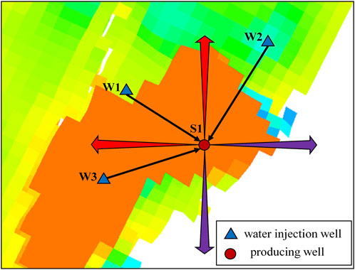
FIGURE 1. Example diagram of reservoir numerical simulation model.
Stable production time, average oil production, recovery rate, water cut rise rate, and production decline rate. First, query and download the production history data of the corresponding sidetracking well from the monthly database of oil well development, plot the oil production curve and water cut curve, and calculate the above indicators according to the following formula:
The formula for calculating average oil production is:
Where
The formula for calculating the recovery rate is:
Where
The formula for calculating the water cut rise rate is:
Where
The formula for calculating the production decline rate is:
Where
In order to explain some complex indicators more intuitively in the above calculation process, such as stable production time, production decline time, terminal water content, initial water content, oil production at the initial stage of decline, and oil production at the end of decline, we have drawn the oil production curve and water cut curve as shown in Figures 2, 3.
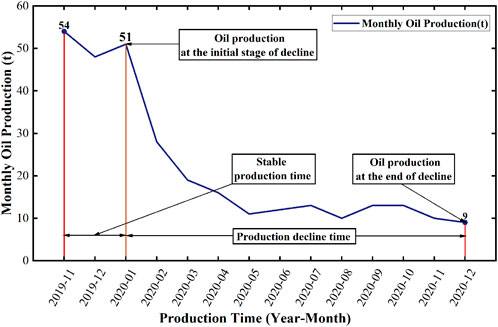
FIGURE 2. S1 oil production curve.
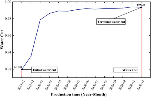
FIGURE 3. S1 water cut curve.
2.3.1 Direct access based on the design book
As shown in Table 3, the influencing factors of residual recoverable reserves and single well control area can be directly obtained from the sidetrack drilling design book.
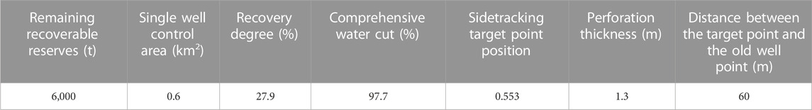
TABLE 3. Data statistics table of the numerical simulation model of S1 well.
2.3.2 Indicator acquisition based on the numerical simulation model
Through investigation of the original numerical simulation model of the target sidetrack drilling well “S1,” it can be known that the original old well opened up strata 21, 22, and 23. Then, data collection and statistics are carried out layer by layer as needed, and according to the statistical results and combined with Formula 1, the index values of oil saturation, permeability, porosity, and the effective thickness of the S1 well can be calculated. Combined with Formulas 2, 3, the variation coefficient and gradient value of permeability, porosity, and effective thickness can be calculated. The specific results are shown in Table 4.
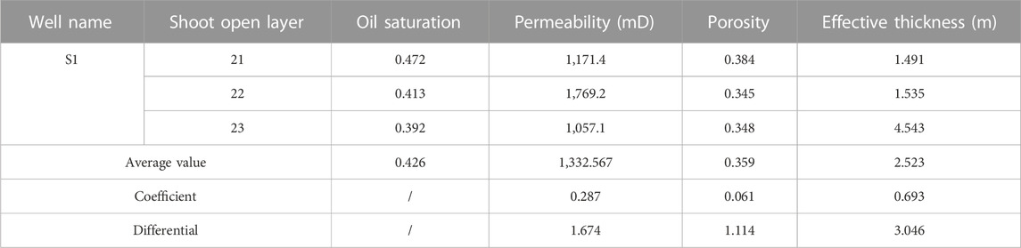
TABLE 4. Initial data statistics table of S1 well numerical simulation model.
From Figure 1, the completeness of the four-direction model of the old well drilled on this side can be judged by whether it is connected. Among them, the purple arrow indicates disconnection, the red arrow indicates connectivity, and the combined Formula 4 shows that the azimuth M of the S1 well connected in this open layer is 2, and the combined Formula 4 can calculate the connection coefficient of the S1 well as 0.5. The larger the connectivity coefficient, the better the connectivity.
In the corresponding well network, the distance between each injection well and the target sidetrack drilling well S1 is counted, and the value of the “injection and production well spacing” of well S1 is calculated in combination with Formula 5 as 178.821.
By observing the position relationship between the target sidetrack drilling well and the surrounding water injection wells in Figure 1, it is judged that the drilling on this side is at the position of the mainstream line or the shunt line. Among them, the main line position is represented by 1, and the shunt line position is represented by 0, that is, the S1 well is located at the shunt line position.
2.3.3 Metric acquisition based on production dynamic datasets
By observing Figure 3, it shows that the oil production of the S1 well began to gradually increase in November 2019 until the production began to decline in January 2020, which shows that the stable production time of the S1 well is 2 months.
According to Figure 3, the cumulative oil production of well S1 from November 2019 to December 2020 is 307 tons, with a total production time of 14 months, and the average oil production of well S1 is 21.929 tons in combination with Formula 6.
Based on the average oil production calculated above, combined with the remaining recoverable reserves value in the original geological parameter index, combined with the calculation method of Formula 7, the value of the recovery rate is 0.044.
Figure 3 shows that the water cut of the S1 well at the beginning and end of production is 91.98% and 99.36%, respectively, combined with the data in the production dynamic data table, the production degree of the S1 well in the early and late production stages is 0.9% and 5.12%, respectively, combined with the calculation method of Formula 8, the value of water cut rise rate is 1.749.
According to Figure 3, the oil production at the end of the decline period, that is, December 2020, is 9 tons, and the production in January 2020 is 51 tons in January 2020, and the decline time is 11 months, and the value of the production decline rate of S1 well can be obtained in combination with Formula 9 as −0.424.
According to the above data statistics method of the S1 well, the actual data of more than 130 sidetrack drilling mines collected are collated, and then the sample set of influencing factors is established. The obtained sample set is cleaned and sorted, and the missing values and outliers in the preliminary obtained data were counted and processed, and the sample set that finally met the research requirements retained the data of 31 sidetrack drilling wells.
3 Influencing factor sensitivity analysis
For the sample set of factors affecting sidetrack drilling, the relationship between each influencing factor and the data parameters of the sidetrack drilling development effect is initially unknown and fuzzy. Therefore, firstly, a single-factor analysis is carried out on each influencing factor and the development effect parameters of sidetrack drilling. The relationship between reservoir geological parameters, sidetrack drilling scheme well design parameters, and sidetrack drilling development effect parameters are qualitatively analyzed by drawing an oil scatter plot. After obtaining a preliminary understanding, Pearson and Spearman correlation analysis methods are used to quantitatively represent the correlation between influencing factors and development effects with correlation coefficients. Based on the above methods, multiple factor analysis is continued to more comprehensively consider the interaction between indicators. Therefore, a feature importance calculation method based on a decision tree is introduced to analyze the importance of each influencing factor on the development effect of sidetrack drilling and sort them.
3.1 Qualitative analysis based on scatter plots
The scatter plot is one of the most commonly used charts in data mining. It can intuitively show the relationship between two continuous variables, including linear and non-linear relationships, increasing and decreasing relationships, and outlier situations (Rajagopalan and Rajagopalan, 2021). When there are multiple quantitative variables with multiple numerical types in the dataset, they can be analyzed by linking each variable together. In this study, the Seaborn tool is used to draw a scatter plot of the impact factor between two factors of a horizontal well and a parameter factor of the horizontal well development effect. Seaborn is a powerful and easy-to-use data visualization tool that is particularly well-suited for drawing high-quality statistical charts. Each point represents an observation sample point (Cihan Sorkun et al., 2022).
Visual analysis of the correlation between 20 influencing factor indicators and 5 different parameters for drilling efficiency in sidetracking wells is conducted using scatter-plots generated by Seaborn’s scatterplot () function. A total of 100 images are produced. Due to space limitations, this paper analyzes and discusses the recovery rate as an example. Figure 4 shows the scatterplot between various influencing factors and the recovery rate.
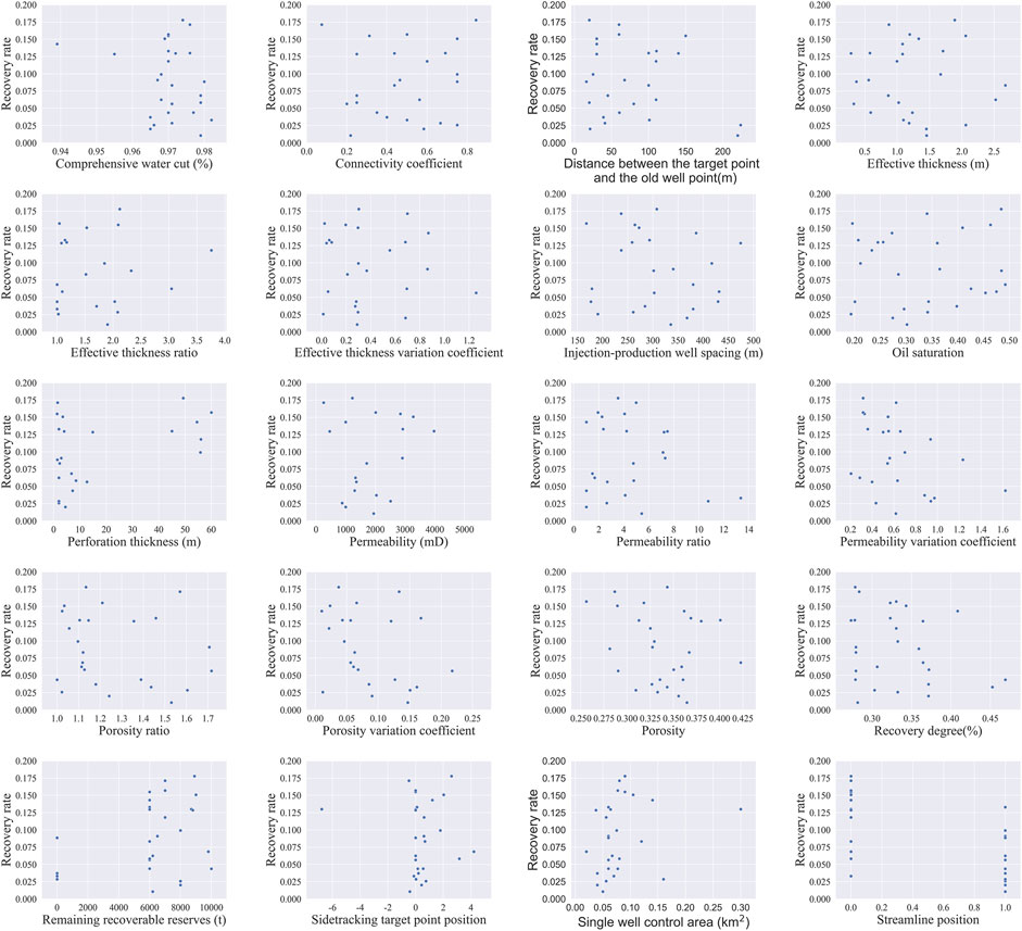
FIGURE 4. Scatter plot between influencing factors and recovery rate.
From Figure 4, it can be seen that the influencing factors such as single well control area, perforation thickness, etc., and recovery rate show a positive correlation, while the influencing factors such as permeability variation coefficient, streamline position, etc., and recovery rate show a negative correlation. However, the overall impact of each influencing factor on the recovery rate of sidetracking wells is not clear enough. This may be because the influence of the indicators of influencing factors on evaluation indicators is not strong enough, or because the relationship between influencing factors and development effect parameters is more complex. Qualitative analysis through visualization alone may not capture clear impact patterns, and further research using other data mining methods is needed to study the relationship between various influencing factor indicators and development effects.
3.2 Quantitative analysis of indicator correlation
From Figure 4, it is difficult to accurately identify the correlation between the influencing factors and the development effect by visualizing scatter plots alone. Therefore, Pearson correlation coefficient and Spearman correlation coefficient analysis methods are used to further analyze the sample set. Pearson correlation coefficient is suitable for data that follows normal distribution or approximate normal distribution, Spearman correlation analysis is mainly used to analyze the relationship between two variables that do not satisfy the normal distribution, or when the variable distribution type is unknown. The Pearson correlation coefficient is mainly used to evaluate linear relationships, while the Spearman correlation coefficient is mainly used to evaluate monotonic relationships (Gu, 2021; Janse et al., 2021).
3.2.1 Pearson correlation
The Pearson correlation coefficient reflects the strength of the linear correlation between the two variables. The higher the absolute value, the stronger the correlation. With different positive and negative shapes, the correlation is also different. This is shown in Table 5.

TABLE 5. Pearson Correlation division.
Through the study of the Pearson correlation, the sample values are substituted for calculation, and the calculation results of the Pearson correlation coefficient between the reservoir geological parameters, the sidetrack drilling design parameters, and the sidetrack drilling development effect parameters are shown in Figure 5.
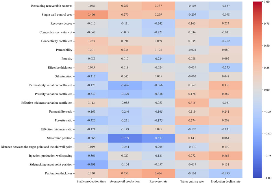
FIGURE 5. Pearson correlation coefficient heat map.
The correlation strength of the variables was judged by the range of the absolute value of the Pearson correlation coefficient after calculation, and the specific evaluation criteria are shown in Table 6.
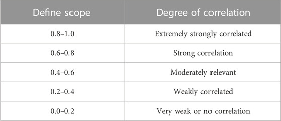
TABLE 6. Correlation coefficient evaluation criteria.
Combining Figure 5; Table 6, it can be seen that 8 indicators are positively correlated with stable production time, and twelve indicators are negatively correlated with stable production time. From the perspective of correlation degree, the absolute value of the correlation coefficient calculated statistically can be found that for eleven indicators such as remaining recoverable reserves and effective thickness, the absolute value of their correlation coefficient is between 0 and 0.2, which belongs to extremely weak correlation; for seven indicators such as connectivity coefficient and permeability, the absolute value of their correlation coefficient is between 0.2 and 0.4, which belongs to weak correlation; for two indicators such as single well control area and sidetracking target point position, the absolute value of their correlation coefficient is between 0.4–0.6, which belongs to moderate correlation. Therefore, a single well control area and sidetracking target point position are indicators that are strongly linearly correlated with stable production time.
Nine indicators are positively correlated with the average oil production and eleven indicators are negatively correlated with it. Among them, ten indicators such as oil recovery degree and comprehensive water cut have an absolute value of correlation coefficient between 0 and 0.2, which belongs to extremely weak correlation; eight indicators such as remaining recoverable reserves and single well control area have an absolute value of correlation coefficient between 0.2 and 0.4, which belongs to weak correlation; one indicator such as permeability variation coefficient has an absolute value of correlation coefficient between 0.4–0.6, which belongs to moderate correlation; one indicator such as streamline position has an absolute value of correlation coefficient between 0.6–0.8, which belongs to strong correlation. Therefore, the permeability variation coefficient and streamline position are indicators that have a strong linear correlation with average oil production.
Seven indicators are positively correlated with the recovery rate, and thirteen indicators are negatively correlated with it. Among them, ten indicators such as connectivity co-efficient and permeability have an absolute value of correlation coefficient between 0 and 0.2, which belongs to extremely weak correlation; eight indicators such as remaining recoverable reserves and single well control area have an absolute value of correlation coefficient between 0.2 and 0.4, which belongs to weak correlation; one indicator such as perforation thickness has an absolute value of correlation coefficient between 0.4–0.6, which belongs to moderate correlation; one indicator such as streamline position has an absolute value of correlation coefficient between 0.6–0.8, which belongs to strong correlation. Therefore, perforation thickness and streamlined position are indicators that have a strong linear correlation with the recovery rate.
Eleven indicators are positively correlated with the water cut rise rate and nine indicators are negatively correlated with it. Among them, sixteen indicators such as remaining recoverable reserves and Recovery degree have an absolute value of correlation coefficient between 0 and 0.2, which belongs to extremely weak correlation; four indicators such as single well control area and coefficient of variation of single effective thickness have an absolute value of correlation coefficient between 0.2 and 0.4, which belongs to weak correlation. Overall, it shows that various geological parameters of oil reservoirs and sidetrack drilling design parameters do not have a significant linear correlation with the water cut rise rate of sidetrack drilling.
Eight indicators are positively correlated with the production decline rate and twelve indicators are negatively correlated with it. Among them, eleven indicators such as remaining recoverable reserves and single well control area have an absolute value of correlation coefficient between 0 and 0.2, which belongs to extremely weak correlation; nine indicators such as Recovery degree and connectivity coefficient have an absolute value of correlation coefficient between 0.2 and 0.4, which belongs to weak correlation. It shows that various geological parameters of oil reservoirs and sidetrack drilling design parameters do not have a significant linear correlation with the production decline rate of sidetracking.
3.2.2 Spearman correlation
The above Pearson correlation analysis is used to measure the linear relationship between two variables. In contrast, Spearman correlation analysis does not require making such an assumption about a linear relationship between the two variables. It involves transforming each variable’s values into ranks and calculating the rank differences between them. Spearman correlation analysis is employed to measure the monotonic relationship between the two variables (Alsaqr, 2021; Hou, 2023).
The formula for calculating Spearman Correlation is:
Where
The calculation process is first to sort the data of the two variables X and Y, and then note the position after sorting (X’, Y’). The value of (X’, Y’) is called a rank. The difference in rank is
Through the study of Spearman’s rank correlation coefficient, the sample values are substituted for calculation, and the Spearman correlation coefficient calculation results between reservoir geological parameters, sidetrack drilling design parameters, and side-track drilling development effect parameters are shown in Figure 6.
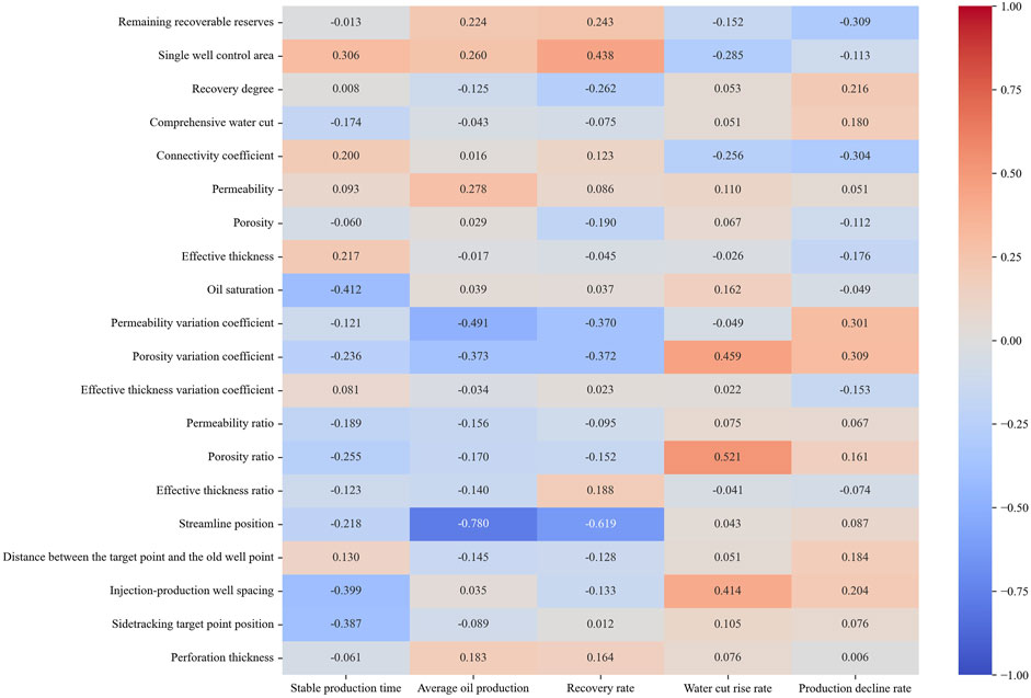
FIGURE 6. Spearman correlation coefficient heat diagram.
According to Figure 6, under the Spearman correlation analysis, the correlation results between the sidetrack drilling development effect parameters and the influencing factors of sidetrack drilling are not much different from the Pearson correlation analysis results, but there are still certain differences. By differentiating the correlation coefficient calculated by Pearson correlation analysis and Spearman correlation analysis, and plotting the heat map as shown in Figure 7 in absolute form, the indicators with large differences are analyzed separately, and the darker the color, the greater the difference.
FIGURE 7. Correlation coefficient difference heat diagram.
According to Figure 7, factors with absolute differences greater than 0.25 are defined as factors with significant differences. Among them, the results of stable production time and average oil production under Pearson and Spearman correlation analysis are relatively similar, and it is believed that the two have a consistent understanding, so it will not be discussed here.
For the recovery rate, the factors with significant differences are perforation thickness, and Figure 4 shows a scatter plot of perforation thickness and recovery rate. The Pearson correlation coefficient between perforation thickness and recovery rate is 0.426, which is moderately correlated, while the Spearman correlation coefficient is 0.164, which is extremely weakly correlated, and the former is significantly higher than the latter. From the scatter plot of perforation thickness and recovery rate, it can be seen that the recovery rate increases with the increase of perforation thickness, showing a positive correlation relationship. Although the Pearson correlation coefficient and Spearman correlation coefficient reflect slightly different degrees of correlation, they both accurately reflect its basic trend.
For the water cut rise rate, the factors with significant differences are the connectivity coefficient, porosity variation coefficient, and effective thickness variation coefficient. For further analysis, Figure 8 shows a scatter plot of the connectivity coefficient, porosity variation coefficient, effective thickness variation coefficient, and water cut. The Pearson correlation coefficient between the connectivity coefficient and water cut is 0.035, while the Spearman correlation coefficient is −0.256. Not only are the two correlation coefficients numerically different, but they also show a reversal of positive and negative correlations. The scatter plot of the connectivity coefficient and water cut shows that the water cut decreases with increasing connectivity coefficient, and the rate of decrease becomes slower and slower, showing a nonlinear negative correlation relationship. Here, the Spearman correlation coefficient more accurately describes it.
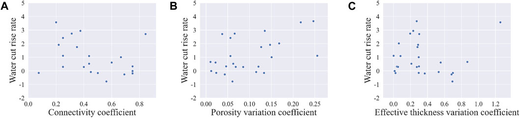
FIGURE 8. Scatter plot of water cut rise rate: (A) Connectivity coefficient- Water cut rise rate scatter plot; (B) Porosity variation coefficient—Water cut rise rate scatter plot; (C) Effective thickness variation coefficient—Water cut rise rate scatter plot.
The Pearson correlation coefficient between the porosity variation coefficient and water cut is 0.178, which is extremely weak, while the Spearman correlation coefficient is 0.459, which is moderately correlated, and the latter calculation result is significantly higher than the former. From the scatter plot of the porosity variation coefficient and water cut, it reflects that the rising rate of water cut shows a certain upward trend with the increase of porosity variation coefficient, but it is not significant and belongs to a weak correlation. Although the Pearson correlation coefficient and Spearman correlation coefficient reflect slightly different degrees of correlation, they both accurately reflect its basic trend.
The Pearson correlation coefficient between the effective thickness variation coefficient and the water cut rise rate is 0.315, which is a weak correlation, and the Spearman correlation coefficient is 0.022, which is a very weak correlation. Although the results are significantly higher than the latter. However, from the scatter plot of the effective thickness variation coefficient and the rising rate of water cut, there is no obvious water cut rise rate and there is a certain upward trend with the increase of effective thickness variation coefficient, but there is no obvious regularity, and the Spearman correlation coefficient here describes it more accurately, so it is more accurate to describe it by combining Pearson correlation coefficient and Spearman correlation coefficient.
For the production decline rate, the Pearson correlation coefficient between perforation thickness and the production decline rate is −0.293, which is a weak correlation, and the Spearman correlation coefficient is 0.006, which is a very weak correlation. The two correlation coefficients not only have a large numerical difference but also have positive and negative reversals. Figure 9 shows the scatter plot of perforation thickness and production decline rate, from which there is no obvious regularity between perforation thickness and production decline rate, whereas the Spearman correlation coefficient describes it more accurately.
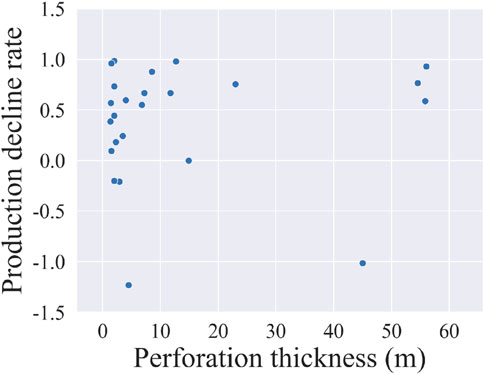
FIGURE 9. Perforation thickness-production decline rate scatter plot.
By comparing the results of the Person correlation analysis and Spearman correlation analysis, it can be found that the Spearman correlation coefficient is more accurate for describing the complex nonlinear correlation between the influencing factors and the sidetrack drilling development effect, so the results of the Spearman correlation analysis are used as the final quantitative characterization results of the correlation between the reservoir geological parameters, the sidetrack drilling design parameters and the sidetrack drilling development effect parameters.
According to the results in Figure 6 and the evaluation criteria in Table 6, the influencing factor that meets the medium correlation degree and above for stable production time is oil saturation; For average oil production, the influencing factors that meet the medium correlation degree and above are the permeability variation coefficient and the streamline position, among which the correlation between the streamline position and the average oil production is the strongest. For recovery rate, the influencing factors that meet the medium correlation degree and above are the control area and streamline position of a single well, among which the streamlined position has the strongest correlation with the recovery rate. For the water cut rise rate, the influencing factors that meet the medium correlation degree and above are porosity variation coefficient, porosity ratio, and injection-production well spacing, among which the correlation between porosity ratio and water cut rise rate is the strongest. For the production decline rate, there are no influencing factors that meet the moderate degree or above, which indicates that the correlation between the production decline rate and the influencing factors is not significant enough, but in general, the index with the strongest correlation with the production decline rate among the influencing factors is the remaining recoverable reserves.
3.3 Ranking analysis of metric importance based on decision trees
Qualitative analysis of the influencing factor sample set and quantitative analysis of the correlation between each influencing factor and the sidetrack drilling development effect parameter is conducted using two single-factor analysis methods, scatter plots, and correlation analysis. These two methods explore the relationship between each influencing factor and the sidetrack drilling development effect factor to some extent. However, single-factor analysis methods have certain limitations. On the one hand, single-factor analysis cannot fully consider the interrelationships between various factors, such as permeability and porosity often showing a strong positive correlation. On the other hand, single-factor analysis is difficult to indicate the size of each influencing factor’s role in the sidetracking development effect. Therefore, further research is needed using multi-factor analysis methods.
With the development of digital oilfields, decision trees have been widely used in economic evaluation, production forecasting, and decision analysis in the petroleum industry as an effective method for processing data sets with complex relationships. At the same time, to explore the degree of influence of geological parameters of oil reservoirs, sidetrack drilling design parameters and other indicators on sidetrack drilling development effect parameters, decision tree algorithms can be used to calculate the importance of each influencing factor on sidetrack drilling development effect parameters and sort the final results. This can intuitively reflect the relationship between various sidetracking influencing factors and sidetracking development effect parameters while fully considering the mutual influence between various factors (Zhou and Hooker, 2021).
The decision tree is a basic classification and regression method. A decision tree consists of nodes and directed edges, with two types of nodes, internal nodes, and leaf nodes. Internal nodes represent a feature or attribute, while leaf nodes represent a category or a value. The decision tree classification algorithm is an instance-based inductive learning method that can extract a tree-like classification model from given unordered training samples. The decision tree model is also a type of white-box model whose prediction results can be explained by humans. We call this feature of machine learning models interpretability, but not all machine learning models have interpretability. As part of the interpretability attribute, feature importance is an indicator that measures the contribution of each input feature to the model’s prediction results.
In a decision tree, each branch represents the result of testing an attribute. The test is represented by each internal node, and each node controls a class label. The decision tree algorithm is based on a top-down recursive divide-and-conquer strategy. The top node of the tree is the root node, representing the first decision. For subsequent decisions, each decision may result in one or more events in their natural state that can produce very different results. Essentially, the decision tree represents a partition of data space. Therefore, decision trees can intuitively show the importance of each attribute to the target attribute (Pappalardo et al., 2021).
For decision trees, in order to measure the importance of features, it is necessary to study how each feature plays a role in the final “decision” of the model. In each split, the final decision (the leaf node) is closer. Therefore, we can say that at each decision node, the chosen segmentation feature determines the final prediction result.
3.3.1 Importance calculation method (DT feature importance)
Specifically, the formula for calculating the importance of the initial characteristics of the decision tree is shown in Formula 11 (Guo et al., 2021).
Where
For the initial feature importance value, it is necessary to normalize the value between 0 and 1 to obtain the final importance value of each feature. For each feature, their importance is a number between 0 and 1, where 0 means “not used at all,” 1 means “perfectly predicted target,” and the sum of the importance of all metric features is always 1.
Taking the decision tree map of Figure 10 as an example, the initial feature importance of the sample indicators X [0], X [1], and X [2] are calculated by using the Formula 11.
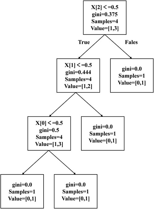
FIGURE 10. A computational instance based on a decision tree map.
Combining the information in Formula 11 and Figure 10, it can be seen that the initial feature importance corresponding to X [0], X [1], and X [2] is respectively:
Normalizing the above results, it can be obtained that the importance of X [0], X [1], X [2] samples
Due to space limitations, the production decline rate is used as an example to analyze and discuss. According to the above calculation method, the calculation results of the importance of ordinary decision trees are shown in Figure 11.
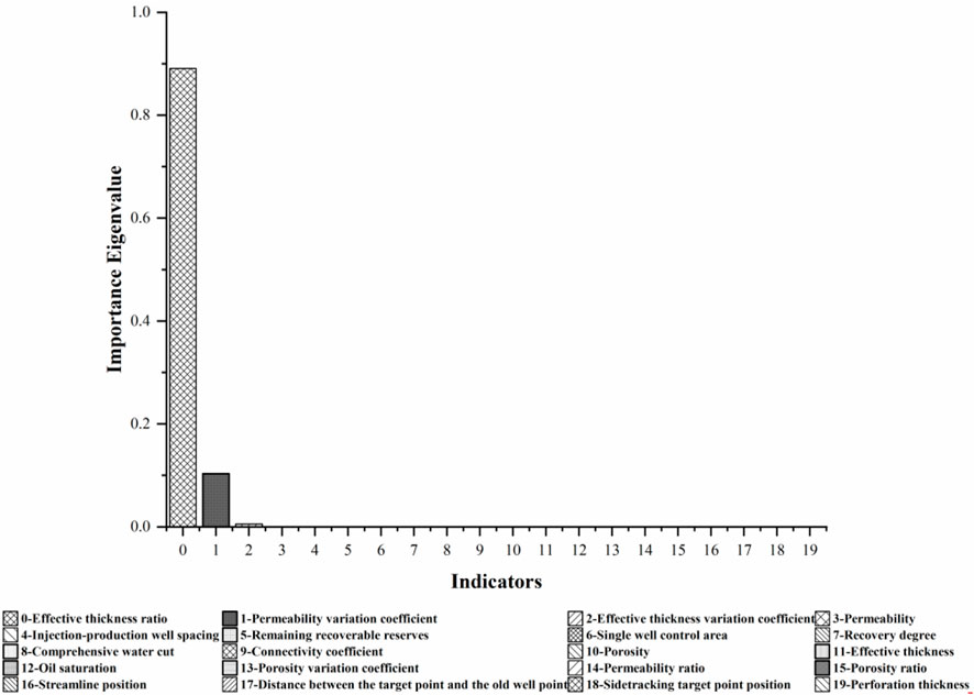
FIGURE 11. Histogram of the importance of each feature under the calculation of the production decline rate in a regular decision tree.
For the production decline rate, the importance ranking of each influencing factor is shown in Figure 11. From the Figure, it can be seen that the effective thickness variation co-efficient accounts for more than 80% of the importance of the production decline rate, while the permeability variation coefficient accounts for more than 10% of its importance. The importance of other indicators is less than 1%. Similar results were obtained for other characteristics of sidetracking development effect parameters, with only one or two indicators accounting for more than 80% of the importance of sidetracking development effect parameters among all influencing factors. This is quite different from theoretical and mining practice knowledge. Analysis believes that this situation may be due to the imbalance of sample data distribution in actual mining field data. Ordinary decision tree models lack effective mechanisms to deal with imbalanced samples, leading to overfitting.
3.3.2 Adaptive enhanced decision trees (Ada feature importance)
In order to alleviate the calculation overfitting caused by the imbalance of the distribution of actual sample data in the mine, the adaptive enhanced decision tree method (AdaBoost) is used to calculate the feature importance of the samples (Panhalkar and Doye, 2022).
The basic principle of the AdaBoost (Adaptive Boosting) algorithm is to reasonably combine multiple weak classifiers (weak classifiers generally use a single-layer decision tree) to make it a strong classifier. The adaptation is that the samples misclassified by the previous basic classifier will be weighted, and the weighted entire sample will be used again to train the next basic classifier, while the weights of the correctly classified samples of the previous round will be reduced. At the same time, a new weak classifier is added to each round until a predetermined sufficiently small error rate is reached or a pre-specified maximum number of iterations is reached. Figure 12 shows the schematic diagram of the adaptive decision tree algorithm (Zhang and Bifet, 2020).
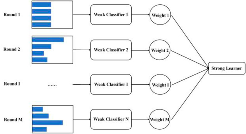
FIGURE 12. Schematic diagram of adaptive enhanced decision trees.
According to Figure 12, the histogram in the leftmost rectangle represents each sample, the different widths represent its weight size, and the weight distribution of the initialized training sample has the same weight; Training a weak classifier, if the sample classification is correct, its weight will be reduced when constructing the next training set; On the contrary, improve. Train the next classifier with the updated sample set; After the training process of each weak classifier is completed, increase the weight of the weak classifier with a small classification error rate and reduce the weight of the weak classifier with a large classification error rate. Compared with ordinary decision tree models, adaptive enhanced decision trees have the advantages of high classification accuracy, and strong flexibility, and are not easy to overfit (Kumari and Sai, 2022).
According to Formula 11, the feature importance of each influencing factor under model training for sidetrack drilling development effect parameters can be obtained according to Formula 11. Similarly, taking the production decline rate as an example, the results of the importance calculation using the adaptive enhanced decision tree method are shown in Figure 12.
According to the results of Figure 13, the importance of each influencing factor to the production decline rate is calculated based on the adaptive enhanced decision tree method, and the top 10 are the permeability variation coefficient, effective thickness variation coefficient, permeability ratio, effective thickness ratio, recovery degree, porosity, the distance between the target point and the old well point, porosity variation coefficient, remaining recoverable reserves, and injection-production well spacing. The combined importance of these top 10 indicators to the production decline rate exceeds 80%.
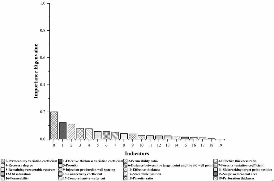
FIGURE 13. Histogram of the importance of each feature in adaptive enhanced decision tree calculation based on production decline rate.
3.3.3 Comprehensive calculation
According to the influencing relationship between the five sidetrack drilling development effect parameters and each influencing factor, the importance calculation method of the adaptive enhanced decision tree is used to calculate the importance between the five sidetrack drilling development effect parameters and their various influencing factors, and the final results are summed and then averaged, which is used as a comprehensive evaluation index to analyze and study the importance of each influencing factor to the sidetrack drilling development effect parameters. Figure 14 shows the ranking results of the feature importance values comprehensively calculated by each influencing factor on the sidetrack drilling development effect parameters.
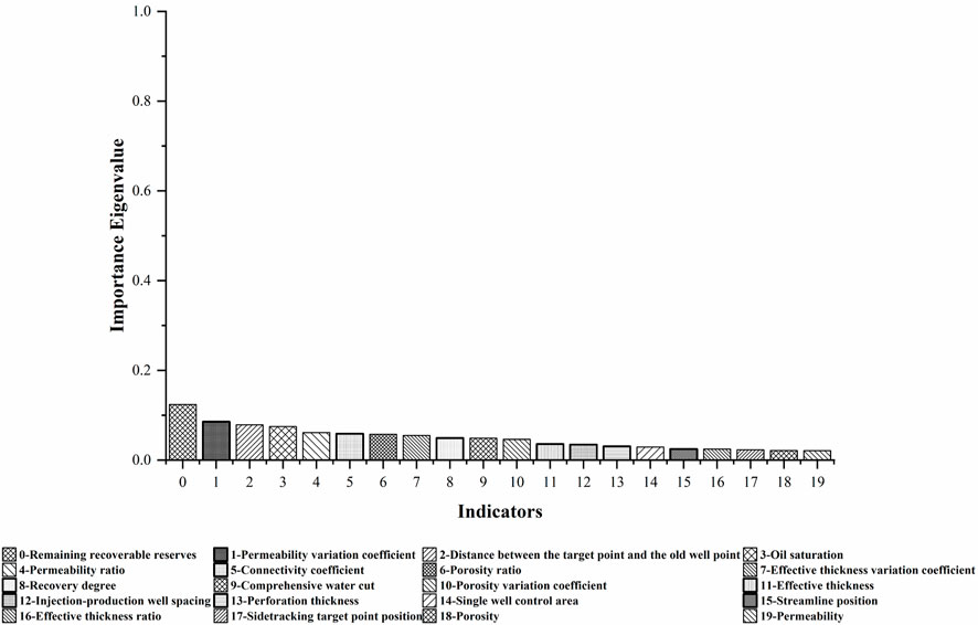
FIGURE 14. Histogram of the importance of each feature in adaptive enhanced decision tree calculation using comprehensive indicators. According to Figure, the characteristic importance of each influencing factor after the calculation of the adaptive enhanced decision tree is the remaining recoverable reserves, the permeability variation coefficient, distance between the sidetracking target point position and the old well point, oil saturation, permeability ratio, comprehensive water cut, porosity ratio, effective thickness variation coefficient, recovery degree, connectivity coefficient, porosity variation coefficient, effective thickness, injection-production well spacing, perforation thickness, single well control area, streamline position, effective thickness ratio, sidetracking target point position, porosity, permeability. Among them, only the remaining recoverable reserves are more than 10% important to the development effect of sidetrack drilling; In addition, the total value of streamline position, effective thickness variation coefficient, sidetracking target point position, porosity, and permeability on the importance of sidetrack drilling development effect only exceeds 10%, which indicates that the above indicators have a weak influence on the importance of sidetrack drilling development effect.
4 Conclusion
This article proposes a study on sensitivity analysis of oil well drilling development effect factors based on actual mining field data. Based on the actual data of more than 130 sidetracking wells in an oil field and combined with expert experience, an influence factor sample set was established. Through three sensitivity analysis methods under single-factor and multi-factor analysis, the value law between geological parameters of oil reservoirs, sidetracking well design parameters, and development effect parameters of sidetracking wells was accurately and objectively described.
In single-factor analysis, scatter plots of each influencing factor and development effect parameters of sidetracking wells are drawn to qualitatively study the relationship between each influencing factor and the development effect of sidetracking wells. The correlation coefficient between each influencing factor and the development effect parameters of sidetracking wells is calculated through Pearson and Spearman correlation analysis methods, which quantitatively characterized the correlation between each influencing factor and the development effect of sidetracking wells. Finally, it is determined that the Spearman correlation analysis method can more accurately describe the complex nonlinear correlation between each influencing factor and development effect parameters of sidetracking wells. The correlation between influencing factors such as oil saturation, permeability variation coefficient, streamline position, single well control area, porosity variation coefficient, porosity ratio, and injection-production well spacing and development effect parameters of sidetracking wells meets a moderate or higher degree of correlation.
To avoid the limitations of using a single-factor analysis, a multi-factor analysis method is used to fully consider the interaction between influencing factors. Based on the calculation method of decision tree feature importance, the self-adaptive enhanced decision tree feature importance calculation method is used to calculate and rank the feature importance of various influencing factor indicators and 5 sidetracking development effect indicator parameters. Among them, only the remaining recoverable reserves have an importance of more than 10% on the sidetracking development effect; in addition, the importance of 6 indicators, such as perforation thickness, is small, all less than 3%.
In this study, we have analyzed the relationship between various influencing factors and the parameters of the development effect of sidetracking wells in a relatively accurate and objective manner. In subsequent studies, more data can be collected sustainably to expand the sample set of influencing factors and continuously improve understanding based on this research method. After capturing certain rules that affect the development effect of sidetrack drilling, the method of association rules can be used to further find efficient development models. On this basis, research on predicting the effect of sidetrack drilling development measures can be carried out.
Data availability statement
The original contributions presented in the study are included in the article/Supplementary Material, further inquiries can be directed to the corresponding author.
Author contributions
XW: Conceptualization, Methodology, Writing—Review and Editing, Supervision, Project administration, Resources, Funding acquisition. CR: Formal analysis, Investigation, Writing—Original Draft, Visualization. HL: Resources, Supervision, Project administration. All authors contributed to the article and approved the submitted version.
Funding
This work has been financially supported by the National Natural Science Foundation of China (No. 52204027), and the Jiangsu Province Postgraduate Research and Practice Innovation Plan Project number (SJCX23_1573).
Acknowledgments
We would like to express our gratitude to the funding provided by the National Natural Science Foundation of China (No. 52204027), and the Jiangsu Province Postgraduate Research and Practice Innovation Plan Project number (SJCX23_1573).
Conflict of interest
Author HL was employed by Sinopec Shengli Oil Field Branch.
The remaining authors declare that the research was conducted in the absence of any commercial or financial relationships that could be construed as a potential conflict of interest.
Publisher’s note
All claims expressed in this article are solely those of the authors and do not necessarily represent those of their affiliated organizations, or those of the publisher, the editors and the reviewers. Any product that may be evaluated in this article, or claim that may be made by its manufacturer, is not guaranteed or endorsed by the publisher.
Supplementary material
The Supplementary Material for this article can be found online at: https://www.frontiersin.org/articles/10.3389/fenrg.2023.1250336/full#supplementary-material
References
Akhmetov, M., Maximov, M., Lymarev, M., et al. (2019). Drilling extended reach well with eight fishbone sidetracks: East Messoyakha Field. OnePetro: SPE Russian Petroleum Technology Conference.
Alsaqr, A. M. (2021). Remarks on the use of Pearson’s and Spearman’s correlation coefficients in assessing relationships in ophthalmic data. Afr. Vis. Eye Health 80 (1), 10. doi:10.4102/aveh.v80i1.612
Chen, Y-H., Li, Y., Hu, D-D., et al. (2021). “Optimized design of horizontal well sidetracking in a porous carbonate reservoir with thief zone,” in International field exploration and development conference (Springer), 189–201.
Cihan Sorkun, M., Mullaj, D., Koelman, J. V. A., and Er, S. (2022). ChemPlot, a Python library for chemical space visualization. Chemistry-Methods 2 (7), e202200005. doi:10.1002/cmtd.202200038
Gao, H. (2023). Influencing factors and measures of water drive oilfield development effect. EDP Sciences: E3S Web of Conferences.01021
Gu, P. (2021). “A study on listening comprehension anxiety in Chinese junior middle school students based on the Pearson correlation analysis,” in 2021 2nd International Conference on Artificial Intelligence and Education (ICAIE), Dali, China, 18-20 June 2021 (IEEE), 332–335.
Guo, Z., Shi, Y., Huang, F., Fan, X., and Huang, J. (2021). Landslide susceptibility zonation method based on C5. 0 decision tree and K-means cluster algorithms to improve the efficiency of risk management. Geosci. Front. 12 (6), 101249. doi:10.1016/j.gsf.2021.101249
Hou, Y. (2023). Analysis of the composition of ancient glass products based on Spearman's correlation coefficient. Highlights Sci. Eng. Technol. 58, 59–65. doi:10.54097/hset.v58i.10026
Janse, R. J., Hoekstra, T., Jager, K. J., Zoccali, C., Tripepi, G., Dekker, F. W., et al. (2021). Conducting correlation analysis: important limitations and pitfalls. Clin. Kidney J. 14 (11), 2332–2337. doi:10.1093/ckj/sfab085
Kumari, L., and Sai, Y. P. (2022). Classification of ECG beats using optimized decision tree and adaptive boosted optimized decision tree. Signal, Image Video Process. 16 (3), 695–703. doi:10.1007/s11760-021-02009-x
Magizov, B., Molchanov, D., Devyashina, A., Tatiana, T., Ksenya, Z., et al. (2021). Multivariant well placement and well drilling parameters optimization methodology. Case study from yamal gas field. SPE Russian Petroleum Technology Conference? : SPE, D041S019R002.doi:10.2118/206574-MS
Panhalkar, A. R., and Doye, D. D. (2022). A novel approach to build accurate and diverse decision tree forest. Evol. Intell. 15 (1), 439–453. doi:10.1007/s12065-020-00519-0
Pappalardo, G., Cafiso, S., Di Graziano, A., and Severino, A. (2021). Decision tree method to analyze the performance of lane support systems. Sustainability 13 (2), 846. doi:10.3390/su13020846
Purbey, R., Parijat, H., Agarwal, D., Mitra, D., Agarwal, R., Pandey, R. K., et al. (2022). Machine learning and data mining assisted petroleum reservoir engineering: A comprehensive review. Int. J. Oil, Gas Coal Technol. 30 (4), 359–387. doi:10.1504/ijogct.2022.124412
Rajagopalan, G., and Rajagopalan, G. (2021). A Python data analyst’s toolkit: Learn Python and Python-based libraries with applications in data analysis and statistics, 243–278.Data visualization with python libraries
Varushkin, S. V., and Khakimova, Z. A. (2018). The design of geological exploration with side track drilling. Perm J. Petroleum Min. Eng. 18 (1), 16–27. doi:10.15593/2224-9923/2018.3.2
Voronin, A., Gilmanov, Y., Eremeev, D., et al. (2017). An analysis of rotary steerable systems for sidetracking in open hole Fishbone multilateral wells in vostochno-messoyakhskoye field. OnePetro: SPE Russian Petroleum Technology Conference.
Wang, S., Liao, G., Zhang, Z., and Wang, X. (2022a). Study on wellbore stability evaluation method of new drilled well in old reservoir. Processes 10 (7), 1334. doi:10.3390/pr10071334
Wang, W., Zhiheng, W., Yulong, M., et al. (2022b). Technologies and application of sidetracking horizontal well in existing wells in sulige gas field. Xinjiang Pet. Geol. 43 (3), 368.
Xu, C., Zhang, H., Kang, Y., Zhang, J., Bai, Y., Zhang, J., et al. (2022). Physical plugging of lost circulation fractures at microscopic level. Fuel 317, 123477. doi:10.1016/j.fuel.2022.123477
Xu, C., Zhang, H., She, J., Jiang, G., Peng, C., and You, Z. (2023). Experimental study on fracture plugging effect of irregular-shaped lost circulation materials. Energy 276, 127544. doi:10.1016/j.energy.2023.127544
Yang, T., Zhang, L., Kim, T., Hong, Y., Zhang, D., and Peng, Q. (2021). A large-scalecomparison of Artificial Intelligence and Data Mining (AI&DM) techniques in simulating reservoir releases over the Upper Colorado Region. J. Hydrology 602, 126723. doi:10.1016/j.jhydrol.2021.126723
Yuan, S., Song, J., Li, L., Jiang, H., and Sun, X. (2022). Numerical simulation study on the development effect of gravity fire flooding by vertical well sidetracking. J. Energy 2022, 1–10. doi:10.1155/2022/5737027
Yuan, Z., Huang, H., Jiang, Y., and Li, J. (2021). Hybrid deep neural networks for reservoir production prediction. J. Petroleum Sci. Eng. 197, 108111. doi:10.1016/j.petrol.2020.108111
Zhang, W., and Bifet, A. (2020). “Feat: A fairness-enhancing and concept-adapting decision tree classifier,” in Proceedings 23 Discovery Science: 23rd International Conference, DS 2020, Thessaloniki, Greece, October 19–21, 2020 (Springer), 175–189.
Keywords: sidetracking well, actual production data, data mining, influencing factors, sensitivity analysis
Citation: Wang X, Rui C and Liu H (2023) Analysis of sensitive factors for sidetrack drilling in water-flooded oil reservoirs: data mining based on actual field data. Front. Energy Res. 11:1250336. doi: 10.3389/fenrg.2023.1250336
Received: 30 June 2023; Accepted: 28 August 2023;
Published: 08 September 2023.
Edited by:
Chengyuan Xu, Southwest Petroleum University, ChinaReviewed by:
Xiaodong Han, China University of Petroleum, ChinaBingyuan Hong, Zhejiang Ocean University, China
Jianchun Xu, China University of Petroleum (East China), China
Copyright © 2023 Wang, Rui and Liu. This is an open-access article distributed under the terms of the Creative Commons Attribution License (CC BY). The use, distribution or reproduction in other forums is permitted, provided the original author(s) and the copyright owner(s) are credited and that the original publication in this journal is cited, in accordance with accepted academic practice. No use, distribution or reproduction is permitted which does not comply with these terms.
*Correspondence: Xiang Wang, eGlhbmd3YW5nQGNjenUuZWR1LmNu