Research on concentrated frequency-dependent parameter model for short overhead transmission lines based on first-order rational function fitting

The impedance of power lines is influenced by geological conditions and skin effect, resulting in frequency-dependent characteristics. In this study, a centralized parameter frequency-dependent line model based on first-order rational function fitting is investigated for short overhead transmission lines. The proposed model incorporates a parallel branch consisting of resistance and inductance obtained through rational function fitting, which mimics the frequency-dependent behavior of the line. The coupling between multiple conductors is represented using controlled sources. Comparative analysis of fitting accuracy and computational efficiency across various orders of rational functions reveals that the first-order rational function fitting offers superior computational efficiency while maintaining high accuracy in the medium and low-frequency range. Simulation results demonstrate that the proposed model, when disregarding wave propagation effects, exhibits comparable accuracy to the distributed parameter line model while achieving higher computational efficiency. Moreover, in transient analysis predominantly influenced by power frequency, the proposed model outperforms the frequency-independent pi(π) line model in terms of accuracy.

1 Introduction

Accurate line models are essential for investigating transient analysis in power systems (Zhou et al., 2021; Hu et al., 2022; Lei et al., 2023). The impedance of transmission lines varies with frequency due to the skin effect and the interaction with the ground under alternating electromagnetic fields, resulting in frequency-dependent characteristics (Mingli and Yu, 2004; Martí and Tavighi, 2017; Chen et al., 2022). Currently, line models commonly used in practice can be classified into fixed parameter models and frequency-dependent parameter models. In general, for steady-state conditions at a fixed frequency, a constant parameter line model can be considered (da Prado et al., 2014; da Silva Lessa et al., 2020). However, for electromagnetic transient processes (including DC components, power frequency components, and various harmonic components), due to the varying resistance and reactance of the transmission line at different frequency components, employing a constant parameter line model for electrical quantity calculations would result in significant errors. This is because the resistance and reactance in the low-frequency range are generally smaller than those in the high-frequency range, and applying fixed parameter line models at power frequency can amplify higher harmonic signals in current responses, leading to substantial waveform distortion (Marti, 1982). Hence, to conduct more accurate electromagnetic transient analysis in power systems, exploring line modeling methods that account for frequency-dependent parameters holds crucial theoretical and practical significance.

The models used for transient simulations of overhead lines can be broadly classified into two categories: concentrated parameter frequency-dependent line models and distributed parameter frequency-dependent line models. In cases where the overhead line is long (over 100 km) and spatial effects need to be taken into account, distributed parameter frequency-dependent line models are recommended. Professor J. Marti from the University of British Columbia proposed the Marti model (Marti, 1982; Marti, 1988), which utilizes a filtering network (RC network) with frequency characteristics that match the line’s characteristic impedance to simulate frequency-dependent parameter lines. Gustavsen introduced the vector fitting method, which offers a more accurate fitting approach for the universal Line Model (ULM) (Gustavsen and Semlyen, 1999; Morched et al., 1999; Gustavsen and Nordstrom, 2007). The ULM has been widely adopted as a fundamental distributed parameter frequency-dependent line model in the Electromagnetic Transients Program (PSCAD/EMTP) (Kocar et al., 2010). On the other hand, when the overhead line is short (within 100 km) and the spatial effects of electromagnetic wave propagation along the line can be neglected, concentrated parameter line models also exhibit high accuracy. Furthermore, due to the shorter computational time required compared to distributed parameter models, concentrated parameter line models offer higher computational efficiency. Therefore, when the investigation does not involve the wave propagation characteristics of the transmission line, the use of concentrated parameter line models is more suitable (Ghazizadeh et al., 2022).

In the field of concentrated parameter frequency-dependent line models, extensive research has been conducted, leading to significant achievements. Reference (Kurokawa et al., 2009) proposed a method for approximating the distributed characteristics of a line parameter model by cascading multiple concentrated parameter line models. Each concentrated parameter line model was connected to an RL parallel network to account for the frequency-dependent characteristics of the line parameters. Further advancements were made in reference (Da Costa et al., 2011), where the adaptability of concentrated parameter line models to higher frequency ranges was investigated by employing a sufficient number of cascaded RL networks. To address the issue of high-frequency oscillations resulting from the cascading of numerous RL networks in references (Kurokawa et al., 2009; Da Costa et al., 2011), reference (De Araújo et al., 2015) designed a low-pass passive filter that was integrated into the equivalent circuit of the concentrated parameter line model. This integration effectively mitigated the oscillation problem. Reference (Colqui et al., 2021) examined the voltage response of multi-cascaded concentrated parameter frequency-dependent line models under various lightning current conditions and demonstrated good agreement with distributed parameter frequency-dependent line models through computational analysis. In the cited references (Kurokawa et al., 2009; Da Costa et al., 2011; De Araújo et al., 2015; Colqui et al., 2021), RL networks were serially connected to concentrated parameter line models to capture the frequency-dependent effects of line parameters. However, in reference (Beerten et al., 2016), an alternative approach was proposed. RL networks were connected in parallel with the concentrated parameter line model to construct a frequency-dependent line model. The applicability of this model to high-voltage direct current lines was analyzed. The concentrated parameter frequency-dependent line models investigated in references (Kurokawa et al., 2009; Da Costa et al., 2011; De Araújo et al., 2015; Beerten et al., 2016; Colqui et al., 2021) involved inserting equivalent circuits obtained from vector fitting calculations into the framework of a constant concentrated parameter line model. These models simulated the wave propagation effects of the line by cascading multiple concentrated parameter line models. Nevertheless, it is important to note that utilizing high-order function vector fitting and cascading multiple concentrated parameter line models can adversely impact computational efficiency and lead to a significant waste of computational resources.

If the transmission line is relatively short (below 100 km) and the impact of wave propagation is negligible, accurate results can be achieved in research that ignores wave propagation characteristics by utilizing low-order rational function fitting. Therefore, the objective of this study is to investigate concentrated parameter frequency-dependent line models using low-order rational function fitting.

Initially, we simulate the frequency-dependent behavior of line parameters by employing a parallel combination of resistors and inductors. The values of the resistors and inductors are determined through rational function fitting. Additionally, controlled sources are used to replicate the coupling relationships between multiple conductors. Subsequently, we analyze the accuracy and efficiency of rational function fitting at different orders. Finally, we evaluate the applicability of the proposed model by constructing a concentrated parameter line model based on first-order rational function fitting in PSCAD.

This paper investigates a concentrated parameter frequency-dependent line model suitable for overhead transmission lines. The accuracy and computational efficiency of rational function fitting with various orders were analyzed. The conclusion drawn is that employing a first-order rational function fitting offers the highest computational efficiency and satisfactory results. In comparison to distributed parameter line models, the proposed line model in this paper exhibits higher computational efficiency, while compared to lumped parameter line models, it attains greater accuracy. Furthermore, an applicability analysis of the concentrated parameter line model fitted with a first-order rational function is conducted, accompanied by quantitative conclusion.

2 Rational function fitting method for line impedance

The Carson’s formula (Carson, 1926) is a fundamental approach for calculating the frequency-dependent impedance of transmission lines. This method requires the input of various constants, including the geometric positions of the line towers, wire radius, and DC resistance.

Figure 1 illustrates the geometric parameters of the line towers, defined within a Cartesian coordinate system. A, B, and C represent the geometric positions of the three-phase conductors at the tower. The X-axis represents the horizontal position, while the Y-axis represents the vertical height. The positions of the three-phase conductors are denoted as P_A = [x_A, y_A], P_B = [x_B, y_B], and P_C = [x_C, y_C], where x_i represents the horizontal coordinate of the conductor, and y_i represents its height above the ground. A_mirror, B_mirror, and C_mirror indicate the mirrored positions of the three-phase conductors with respect to the ground. By utilizing the coordinates of the three-phase conductors, the distances d_ij and the mirror distances d_ij,mir (where i, j = A, B, C, and i ≠ j) between the conductors can be calculated. The symbol r_i represents the radius of the conductor, while SAG refers to the conductor sag. By utilizing the sag and the height of the conductor on the tower, denoted as y_i, the average height of the conductor above the ground, denoted as h_i, can be calculated as shown in Eq. 1.

$h_i=\left|y_i\right|-SAG+\frac{1}{3}SAG=\left|y_i\right|-\frac{2}{3}SAG\left(i=A,B,C\right)(1)$

FIGURE 1

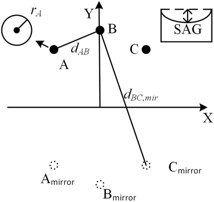
FIGURE 1. Equivalent geometric parameters of overhead lines.

By employing this data, the Carson’s formula can be used to compute the impedance matrix of the transmission line at a specific frequency, as expressed in Eq. 2.

$Z=\left[\begin{array}{ccc}{Z}_{\mathrm{a}\mathrm{a}}& Z_{ab}& Z_{ac}\\ Z_{bc}& Z_{bb}& Z_{bc}\\ Z_{ac}& Z_{bc}& Z_{cc}\end{array}\right](2)$

Reference (Li and Lv, 2019) presents a method to derive the geometric parameters of a line by utilizing the known impedance matrix and capacitance matrix at power frequency. Further, the Carson’s formula is employed to determine the line parameters at different frequencies. To cover a frequency range of 10 ^ -3∼10 ^ 4 Hz, m frequency values, denoted as f(n) (n = 1, 2, m), are selected with a logarithmic uniform distribution. This method enables the calculation of the line impedance matrix, Z(f(n)), corresponding to each of the chosen frequency values.

$\begin{array}{l}Z\left(f\left(n\right)\right)=\left[\begin{array}{ccc}{Z}_{\mathrm{a}\mathrm{a}}\left(f\left(n\right)\right)& Z_{ab}\left(f\left(n\right)\right)& Z_{ac}\left(f\left(n\right)\right)\\ Z_{bc}\left(f\left(n\right)\right)& Z_{bb}\left(f\left(n\right)\right)& Z_{bc}\left(f\left(n\right)\right)\\ Z_{ac}\left(f\left(n\right)\right)& Z_{bc}\left(f\left(n\right)\right)& Z_{cc}\left(f\left(n\right)\right)\end{array}\right]\\ \left(n=\mathrm{1,2}\cdots m\right)\end{array}(3)$

This study does not consider the asymmetric conditions of three-phase lines and specifically focuses on uniformly transposed three-phase lines. Under this assumption, the impedance matrix can be expressed as follows:

$Z=\left[\begin{array}{ccc}{Z}_s& Z_m& Z_m\\ Z_m& Z_s& Z_m\\ Z_m& Z_m& Z_s\end{array}\right](4)$

The Coulomb-Born phase transformation matrix (Liang and Zhu, 2019) was chosen for this study.

$\mathbf{S}=\left[\begin{array}{ccc}1& 1& 1\\ 1& -2& 1\\ 1& 1& -2\end{array}\right](5)$

The matrix (4) is diagonalized by employing Eq. 5:

$Z_{\mathrm{mod}}={\mathbf{S}}^{-1}Z\mathbf{S}=\left[\begin{array}{ccc}{Z}_s+2Z_m& 0& 0\\ 0& Z_s-Z_m& 0\\ 0& 0& Z_s-Z_m\end{array}\right](6)$

At this stage, the zero-sequence impedance and positive-sequence impedance can be expressed as follows:

$\left\{\begin{array}{l}{Z}_0=Z_s+2Z_m\\ Z_1=Z_s-Z_m\end{array}\right.(7)$

By substituting the impedance values at different frequencies from Eq. 3 into Eqs 4–7, we can obtain the following results:

$\begin{array}{l}\left\{\begin{array}{l}{Z}_0\left(f\left(n\right)\right)=Z_s\left(f\left(n\right)\right)+2Z_m\left(f\left(n\right)\right)\\ Z_1\left(f\left(n\right)\right)=Z_s\left(f\left(n\right)\right)-Z_m\left(f\left(n\right)\right)\end{array}\right.\\ n=\mathrm{1,2}\cdots m\end{array}(8)$

Due to the complexity of the Carson’s formula, obtaining a frequency-domain analytical expression is challenging. Hence, we propose utilizing simple rational functions to fit the modulus impedance values obtained from the Carson’s formula at different frequencies (i.e., Eq. 8). By obtaining fitting functions that capture the frequency-dependent characteristics, we can approximate the frequency-domain behavior of the modulus impedance and develop a frequency-dependent line parameter model. Currently, there are two primary types of fitting functions for rational function approximation of impedance, expressed by Eqs 9, 10:

$Z_{fit1}\left(j\omega \right)=R_1+L_{1}j\omega +{\displaystyle \sum _{k=2}^n}\frac{R_{k}j\omega }{j\omega +\left(R_k/L_k\right)}(9)$

$Z_{fit2}\left(j\omega \right)=R_1+{\displaystyle \sum _{k=2}^n}\frac{1/C_k}{j\omega +\left(1/C_k{R}_k\right)}(10)$

In Eqs 9, 10, the coefficients R_k, L_k, C_k (k = 1,2, n) represent the unknown parameters of the fitting functions. These equations can be equivalently represented by the circuit diagrams shown in Figures 2A, B, respectively.

FIGURE 2

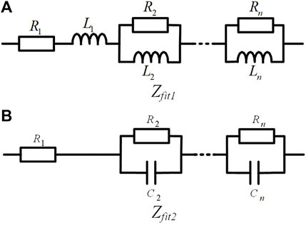
FIGURE 2. Equivalent circuit diagrams of the fitting functions.

These two fitting functions are mathematically similar and exhibit comparable fitting accuracy. In this study, we employ the fitting function Z_fit1, as represented by Eq. 9 and illustrated in Figure 2A, as the equivalent circuit model.

It is important to note that the fitting functions proposed in this study are specifically designed to fit the modulus impedance. In computational and simulation analyses of multi-conductor lines, modulus operations are commonly used. If the fitting target were the complex impedance (Zs, Zm), although the rational function in Eq. 9 is of order (n-1), the modulus impedance (Z₀, Z₁) calculated using Eq. 7 would be of order 2(n-1). Conversely, when directly fitting the modulus impedance, the order of the rational function for the modulus impedance would be (n-1). Therefore, fitting the modulus impedance can reduce the order of the rational function, thereby reducing computational complexity and improving computational speed.

Let the relative deviation between each data point in Eq. 8 and the fitting function in Eq. 9 be denoted as

${\delta }_n=\left|\frac{Z\left(f\left(n\right)\right)-Z_{fit}\left(j2\pi f\left(n\right)\right)}{Z\left(f\left(n\right)\right)}\right|,n=,\mathrm{1,2}\cdots m(11)$

The sum of squared relative deviations is given by:

$J={\displaystyle \sum _{j=1}^m}{{\delta }_n}^2(12)$

Based on the principle of minimizing the sum of squared deviations, the optimal fitting curve Z_fit is obtained using the least squares method. In this study, the forminsearch function in MATLAB is used for implementation.

Upon reaching this stage, the fitting functions Z_fit,x (x = 1,2) can be employed to substitute the modulus impedance Z_x (x = 1,2) calculated using the Carson’s formula.

To validate the accuracy of the proposed fitting functions, a frequency-dependent model of a 10 km three-phase overhead line is constructed in the PSCAD/EMTDC simulation environment, as depicted in Figure 3.

FIGURE 3

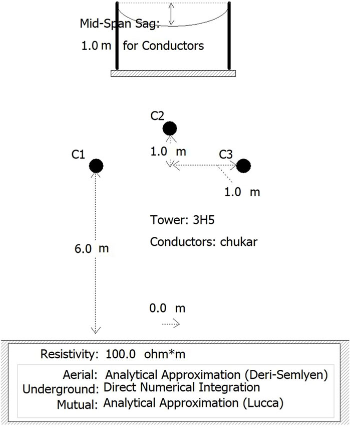
FIGURE 3. Tower structure of three-phase overhead transmission power line.

The tower parameters are set as follows: PA = [-1 m, 6 m], PB = [0 m, 7 m], and PC = [1 m, 6 m]. The SAG is set to 1 m, while the wire radius r_i is chosen as 0.0203454 m. The DC resistance of the wire is determined to be 0.03206 Ω/km. A three-phase balanced transposition scheme is implemented. Subsequently, the line’s modulus impedance parameters obtained from simulations at different frequencies are extracted for comparison with the values calculated using the Carson’s formula and the fitting functions proposed in this study. Initially, a first-order rational function fitting approach is employed, specifically with n = 2 in Eq. 9. The results obtained are depicted in Figures 4, 5.

FIGURE 4

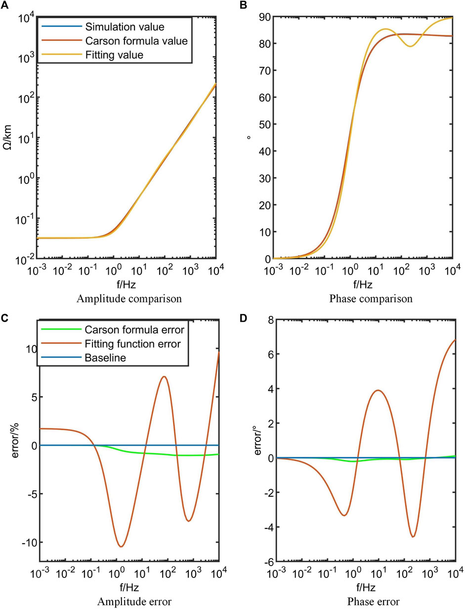
FIGURE 4. Comparison and error analysis of first-order rational function fitting for Z₀.

FIGURE 5

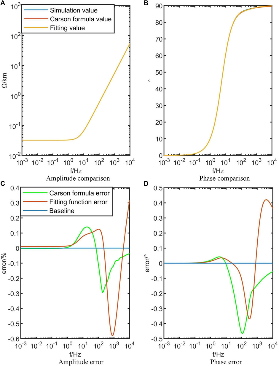
FIGURE 5. Comparison and error analysis of first-order rational function fitting for Z₁.

Figures 4A, B show the comparison between the PSCAD simulated values, the calculated values from the Carson’s formula, and the fitting function approximations for the zero-sequence impedance. Figures 4C, D depict the calculation errors of the Carson’s formula and the fitting function, respectively, based on the precise values obtained from the PSCAD simulations. Similarly, Figure 5 represents the positive-sequence impedance.

Figures 4, 5 demonstrate that the calculated values obtained from the Carson’s formula exhibit remarkable accuracy when compared to the PSCAD simulated values. Furthermore, the first-order rational function approximation yields highly accurate fitting results. Regarding the fitting values, the average magnitude error of the zero-sequence impedance Z0 is 2.95%, with a maximum error of 10.43%. The average phase deviation is 1.82°, with a maximum deviation of 6.83°. Similarly, for the positive-sequence impedance Z1, the average magnitude error is 0.09%, with a maximum error of 0.58%. The average phase deviation is 0.08°, with a maximum deviation of 0.43°. Therefore, it can be concluded that the results obtained from the first-order rational function approximation are highly accurate.

In order to enhance the fitting accuracy, a higher-order rational function approximation can be utilized. Similar to the approach used for the first-order rational function approximation, the error function for the third-order rational function approximation is defined with k = 4 in Eq. 9. Similarly, the error function for the fifth-order rational function approximation is defined k = 6 in Eq. 9. The fitting process was conducted using MATLAB on a desktop computer with an i7-7700 CPU and 12 GB RAM. The first-order approximation required a time of 0.1300 s, the third-order approximation took 0.4775 s, and the fifth-order approximation took 0.9665 s. The efficiency of the first-order rational function approximation is 3.67 times higher than that of the third-order approximation and 7.43 times higher than that of the fifth-order approximation. Figures 6, 7 illustrate the fitting errors of the third-order and fifth-order rational function approximations.

FIGURE 6

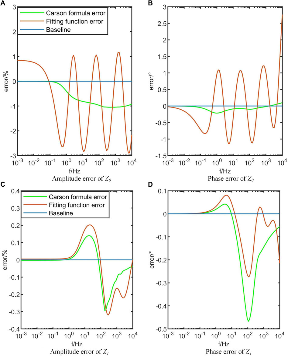
FIGURE 6. Error of third-order fitting function.

FIGURE 7

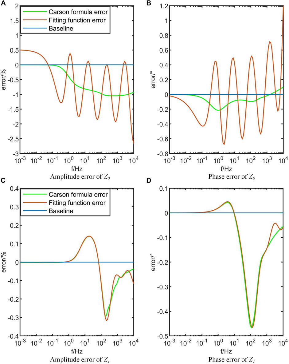
FIGURE 7. Error of fifth-order fitting function.

In Figures 6, 7, the average magnitude error of the zero-sequence impedance obtained from the third-order rational function approximation is 0.91%, with an average phase deviation of 0.55°. For the positive-sequence impedance, the average magnitude error is 0.96%, with an average phase deviation of 0.04°. Regarding the fifth-order rational function approximation, the average magnitude error of the zero-sequence impedance is 0.55%, with an average phase deviation of 0.32°. For the positive-sequence impedance, the average magnitude error is 0.04%, with an average phase deviation of 0.08°. The results in Figures 6, 7 demonstrate that increasing the order of the fitting function can improve the fitting accuracy. However, it is important to note that since the fitting is performed against the values computed by the Carson’s formula, which inherently includes some degree of error, using higher-order fitting functions only leads to a closer approximation of the Carson’s formula values without a significant improvement in fitting function errors.

Given the low computational complexity and ease of implementation, as well as the reasonably accurate fitting results achieved with the first-order rational function approximation method, our subsequent research will predominantly concentrate on its further exploration and refinement.

3 Concentrated-parameter frequency-dependent line model based on the pi(π) line model

In the case of relatively short transmission lines, where the wave propagation characteristics can be neglected, a simplified pi(π) line model is commonly employed as an appropriate line model (Xu et al., 2019). Figure 8 depicts the simplified equivalent circuit of the multi-phase pi(π) line model, which effectively captures the fundamental characteristics of the system.

FIGURE 8

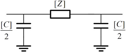
FIGURE 8. Simplified multi-phase pi(π)-type equivalent circuit.

In Figure 8, the impedance matrix for the three-phase balanced interchanged line is represented by Eq. 4, whereas the capacitance matrix is described by Eq. 13.

$\left[C\right]=\left[\begin{array}{ccc}{C}_s& C_m& C_m\\ C_m& C_s& C_m\\ C_m& C_m& C_s\end{array}\right](13)$

The line capacitance typically does not change with varying frequencies (Martinez et al., 2005). In this study, we directly utilize the capacitance values derived from PSCAD simulations for subsequent computational analyses.

Eq. 14 can be derived from Eq. 7.

$\left\{\begin{array}{l}{Z}_s=\frac{1}{3}{Z}_0+\frac{2}{3}{Z}_1\\ Z_m=\frac{1}{3}{Z}_0-\frac{1}{3}{Z}_1\end{array}\right.(14)$

By substituting the obtained first-order fitting functions Z_fit,0(j2πf) and Z_fit,1(j2πf) (derived from Eq. 9 with n = 2) for Z₀ and Z₁ in Eqs 14–16 can be derived.

$\begin{array}{l}{Z}_s=\frac{1}{3}\left(R_{\mathrm{0,1}}+L_{\mathrm{0,1}}j2\pi f+\frac{R_{\mathrm{0,2}}j2\pi f}{j2\pi f+\left(R_{\mathrm{0,2}}/L_{\mathrm{0,2}}\right)}\right)\\ +\frac{2}{3}\left(R_{\mathrm{1,1}}+L_{\mathrm{1,1}}j2\pi f+\frac{R_{\mathrm{1,2}}j2\pi f}{j2\pi f+\left(R_{\mathrm{1,2}}/L_{\mathrm{1,2}}\right)}\right)\\ =R_{s,1}+L_{s,1}j2\pi f+\frac{R_{s,2}j2\pi f}{j2\pi f+\left(R_{s,2}/L_{s,2}\right)}+\frac{R_{s,3}j2\pi f}{j2\pi f+\left(R_{s,3}/L_{s,3}\right)}\end{array}(15)$

$\begin{array}{l}{Z}_m=\frac{1}{3}\left(R_{\mathrm{0,1}}+L_{\mathrm{0,1}}j2\pi f+\frac{R_{\mathrm{0,2}}j2\pi f}{j2\pi f+\left(R_{\mathrm{0,2}}/L_{\mathrm{0,2}}\right)}\right)\\ -\frac{1}{3}\left(R_{\mathrm{1,1}}+L_{\mathrm{1,1}}j2\pi f+\frac{R_{\mathrm{1,2}}j2\pi f}{j2\pi f+\left(R_{\mathrm{1,2}}/L_{\mathrm{1,2}}\right)}\right)\\ =R_{m,1}+L_{m,1}j2\pi f+\frac{R_{m,2}j2\pi f}{j2\pi f+\left(R_{m,2}/L_{m,2}\right)}+\frac{R_{m,3}j2\pi f}{j2\pi f+\left(R_{m,3}/L_{m,3}\right)}\end{array}(16)$

In the above equations, R_s,x, L_s,x, R_m,x, and L_s,x (x = 1,2,3) represent the combined terms. The equivalent circuit diagrams for Z_s and Z_m are shown in Figure 9.

FIGURE 9

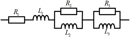
FIGURE 9. Equivalent circuit diagrams of Z_s and Z_m.

4 Simulation verification

To validate the proposed approach, a simulation model was constructed in the PSCAD/EMTDC environment, replicating the same line model as described in Section 2. The geometric parameters of the overhead line were incorporated into the Carson’s formula to calculate the line parameters. Subsequently, based on the methodology outlined in Section 3, all parameters for the fitting functions Z_s and Z_m were computed and their corresponding values are presented in Table 1.

TABLE 1

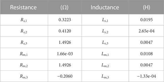
TABLE 1. Parameters in the fitting functions Z_s and Z_m.

Using the data provided in Table 1, a centralized parameter frequency-dependent transmission line model is constructed in the PSCAD/EMTDC simulation environment, as illustrated in Figure 10. The coupling between multiple conductors is simulated using controlled sources to accurately represent the relationship described by Eq. 17.

$\left[\begin{array}{l}{u}_a\\ u_b\\ u_c\end{array}\right]=\left[\begin{array}{ccc}{Z}_s& Z_m& Z_m\\ Z_m& Z_s& Z_m\\ Z_m& Z_m& Z_s\end{array}\right]\left[\begin{array}{l}{i}_a\\ i_b\\ i_c\end{array}\right](17)$

FIGURE 10

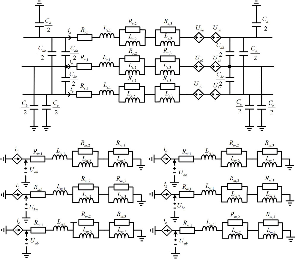
FIGURE 10. Centralized parameter frequency-dependent transmission line model built in PSCAD.

A comparative analysis is conducted to investigate the current responses of the proposed centralized parameter frequency-dependent line model (CPLM) and the distributed parameter frequency-dependent line model (DPLM) in PSCAD at different voltage frequencies. The line length is set to 10 km, and the leading terminal of the line is subjected to 10 kV voltages at various frequencies, while the other end is directly grounded (without load connection to assess the accuracy of the line model). The current response at the leading terminal of the line is measured, as shown in Figure 11.

FIGURE 11

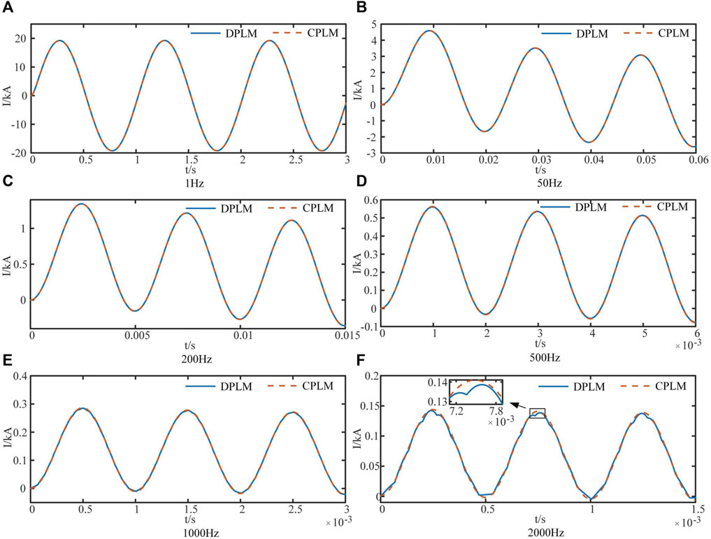
FIGURE 11. Line current response at different frequency voltages.

When the length of the line is 10 km, Figures 11A–E demonstrate a high level of consistency, below 1,000 Hz, between the proposed centralized parameter frequency-dependent line model in this study and the distributed parameter frequency-dependent line model. However, Figure 11F reveals a significant difference in the circuit response between the proposed model and the distributed parameter model at 2000 Hz.

In order to analyze the limiting frequency for various line lengths while maintaining accuracy, this study conducted additional current response simulations for line lengths of 200 km, 100 km, 10 km, and 1 km at different voltage frequencies, as illustrated in Figure 12.

FIGURE 12

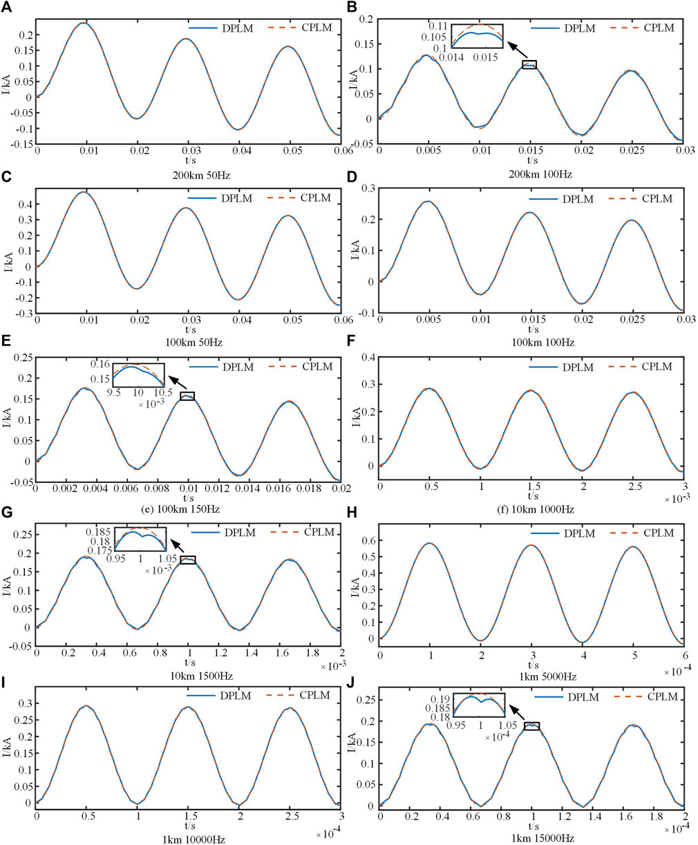
FIGURE 12. Response of different length lines under different frequency voltages.

From Figures 12A, B, it is evident that for a transmission line length of 200 km, the model’s accuracy is relatively high when considering only the power frequency (50 Hz) electrical quantity. However, the model’s precision noticeably decreases when the frequency exceeds 100 Hz. Figures 12C–E demonstrate that for a transmission line length of 100 km, the model is more accurate when the frequency is below 100 Hz, and its accuracy decreases noticeably when the frequency exceeds 150 Hz (third harmonic). Similarly, Figures 12F, G, and Figure 11 indicate that for a transmission line length of 10 km, the model is more accurate when the frequency is below 1,000 Hz, and its accuracy decreases significantly when the frequency surpasses 1,500 Hz. Moreover, Figures 12H–J show that for a transmission line length of 1 km, the model achieves higher accuracy when the frequency is below 10,000 Hz and experiences a noticeable decline in accuracy when the frequency exceeds 15,000 Hz.

According to reference (Cui et al., 2019), it has been observed that the accuracy of the concentrated parameter transmission line model is higher when the line length is much smaller than the electromagnetic wave’s wavelength. The formula for calculating the wavelength (λ) is as follows:

$\lambda =\frac{c}{f}(18)$

where λ represents the wavelength, c is the speed of light (typically taken as 3 × 10^8 m/s), and f is the frequency. Setting the ratio (k) between the electromagnetic wave’s wavelength (λ) and the line length (l) as:

$k=\frac{\lambda }{l}(19)$

Based on simulations, the following conclusion can be drawn: When k is greater than 30, our model is relatively accurate, while when k is less than 20, the model’s precision noticeably declines.

If we consider only the power frequency (50 Hz), we believe that the maximum distance for our transmission line model is 200 km, as it still ensures accuracy for power frequency (50 Hz) electrical quantities at that distance. If we also consider the third harmonic (150 Hz), we consider 66.7 km as the maximum distance, ensuring accuracy for third harmonic electrical quantities at that distance. If readers want to explore the limiting distance for different frequencies or the limiting frequency for different line lengths, they can use Formulas (18) and (19) for calculations.

The following section presents an analysis of the current responses in a three-phase line under normal operating conditions with a load at the industrial frequency of 50 Hz. Specifically, we examine the current responses at the 0.1-s mark for two fault scenarios: single-phase-to-ground fault and two-phase-to-ground fault at the far end of the line. These faults are characterized by zero-resistance short circuits, which are idealized to emphasize the accuracy of the line parameters. To evaluate the performance of our proposed centralized parameter frequency-dependent line model (CPLM), we compare it with two benchmark models: the distributed parameter frequency-dependent line model (DPLM) implemented in PSCAD and the widely used pi(π) line model (πLM). The comparative analysis is depicted in Figure 13.

FIGURE 13

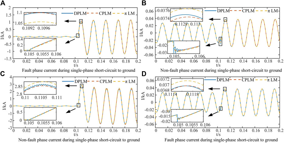
FIGURE 13. Current waveforms under different short circuit faults.

In Figure 13, by considering the PSCAD distributed parameter frequency-dependent line model (DPLM) as the accurate reference model, the following conclusions can be drawn: for a 10 km long line, when disregarding the wave propagation effect, the utilization of the proposed centralized parameter frequency-dependent line model based on the first-order rational function fitting yields higher accuracy in estimating the transient short-circuit current primarily driven by the power frequency, compared to the conventional pi(π) line model.

5 Conclusion

This study presents an investigation into a novel centralized parameter frequency-dependent line model based on first-order rational function fitting. The proposed model offers an efficient simulation approach for capturing the behavior of medium-to-low frequency responses in three-phase or two-phase overhead lines while neglecting the wave propagation effects. The conclusions and contributions of this paper are as follows:

1) This study analyzes the accuracy and computational efficiency of rational function fitting with different orders for estimating line impedance. The following conclusions are drawn: The computational efficiency of the first-order rational function fitting is 3.67 times higher than that of the third-order fitting and 7.43 times higher than that of the fifth-order fitting. Moreover, when considering only the medium-to-low frequency range, the first-order fitting exhibits comparable accuracy to higher-order fittings.

2) The proposed line model in this paper offers higher computational efficiency compared to the distributed parameter line model. Specifically, without considering wave propagation characteristics, the proposed model demonstrates higher accuracy. In the context of power-frequency-dominated electromagnetic transient processes, the proposed model outperforms the centralized parameter pi(π) model in terms of accuracy.

3) An applicability analysis is conducted for the centralized parameter line model utilizing first-order rational function fitting. The results indicate that when the ratio k between the electromagnetic wave wavelength λ and the line length l exceeds 30, this line model demonstrates a high level of accuracy. Conversely, when k falls below 20, the accuracy of the line model diminishes.

This paper focuses on the frequency-dependent model for overhead lines, while the frequency-dependent model for cables requires further investigation. The concatenation of multiple lumped parameter line models can overcome the length limitation of conductors and simulate wave propagation effects. The application of lumped parameter line models for calculating wave propagation and whether tuning wave protection using such model could potentially outperform the existing wave protection methods are subjects that warrant further research.

Data availability statement

The original contributions presented in the study are included in the article/Supplementary material, further inquiries can be directed to the corresponding author.

Author contributions

BL wrote the manuscript. MS and WW organized case studies. XJ and FX contributed to the theoretical research of this manuscript. All authors contributed to the article and approved the submitted version.

Funding

This work is supported by the State Grid Corporation of China Headquarters Science and Technology Project (No. 5400-202122573A-0-5-SF).

Conflict of interest

Authors XJ and FX were employed by State Grid Hubei Electric Power Co., Ltd.

The remaining authors declare that the research was conducted in the absence of any commercial or financial relationships that could be construed as a potential conflict of interest.

The authors declare that this study received funding from the State Grid Corporation of China. The funder had the following involvement in the study: study design, data collection, analysis, and interpretation.

Publisher’s note

All claims expressed in this article are solely those of the authors and do not necessarily represent those of their affiliated organizations, or those of the publisher, the editors and the reviewers. Any product that may be evaluated in this article, or claim that may be made by its manufacturer, is not guaranteed or endorsed by the publisher.

References

Beerten, J., D'Arco, S., and Suul, J. A. (2016). Frequency-dependent cable modelling for small-signal stability analysis of VSC-HVDC systems. IET Gener. Transm. Distrib. 10 (6), 1370–1381. doi:10.1049/iet-gtd.2015.0868

CrossRef Full Text | Google Scholar

Carson, J. R. (1926). Wave propagation in overhead wires with ground return. Bell Syst. Tech. J. 5 (4), 539–554. doi:10.1002/j.1538-7305.1926.tb00122.x

CrossRef Full Text | Google Scholar

Chen, S., Li, B., Liu, T., He, C., Zhang, M., and Wang, T. (2022). Mpedance modeling of DC grid considering the frequency-dependent characteristics of cable and overhead line parameters. Electr. Power Eng. Technol. 41 (06), 101–108. doi:10.12158/j.2096-3203.2022.06.012

CrossRef Full Text | Google Scholar

Colqui, J. S. L., Timaná, L. C., Kurokawa, S., De Araújo, A. R. J., and Pissolato Filho, J. (2021). “Lightning current on the frequency-dependent lumped parameter model representing short transmission lines,” in 2021 35th International Conference on Lightning Protection (ICLP) and XVI International Symposium on Lightning Protection (SIPDA), Colombo, Sri Lanka, 20-26 September 2021 (IEEE), 1–8.

Google Scholar

Cui, K., Wen, J., Zhao, X., Xin, Q., Wei, Z., and Han, M. (2019). Flexibly segmented non-decoupling algorithm for frequency-dependent model of multi-phase coupled transmission line. Proc. CSEE 39 (08), 2307–2314+13. doi:10.13334/j.0258-8013.pcsee.171744

CrossRef Full Text | Google Scholar

Da Costa, E. C. M., Kurokawa, S., do Prado, A. J., and Pissolato, J. (2011). Proposal of an alternative transmission line model for symmetrical and asymmetrical configurations. Int. J. Electr. Power Energy Syst. 33 (8), 1375–1383. doi:10.1016/j.ijepes.2011.06.015

CrossRef Full Text | Google Scholar

da Silva Lessa, L., de Luca, C. C. S., Pereira, T. G., Grilo, C. V. C., Moreira, A. C., Ronchini, C. M. B., et al. (2020). Sparse matrices for transient simulations with computing memory reduction. Electr. Power Syst. Res. 183, 106266. doi:10.1016/j.epsr.2020.106266

CrossRef Full Text | Google Scholar

De Araújo, A. R. J., Da Silva, R. C., and Kurokawa, S. (2015). Reducing the´ spurious oscillations in the lumped parameters model using low-pass filter. IEEE Lat. Am. Trans. 13 (4), 1029–1034. doi:10.1109/tla.2015.7106353

CrossRef Full Text | Google Scholar

do Prado, A. J., da Silva Lessa, L., Monzani, R. C., Bovolato, L. F., and Pissolato Filho, J. (2014). Modified routine for decreasing numeric oscillations at associations of lumped elements. Electr. Power Syst. Res. 112, 56–64. doi:10.1016/j.epsr.2014.03.006

CrossRef Full Text | Google Scholar

Ghazizadeh, M., Ajaei, F. B., and Dounavis, A. (2022). Passive lumped DC line model with frequency-dependent parameters for transient studies. IEEE Trans. Power Deliv. 37 (5), 3947–3957. doi:10.1109/tpwrd.2022.3141706

CrossRef Full Text | Google Scholar

Gustavsen, B., and Nordstrom, J. (2007). Pole identification for the universal line model based on trace fitting. IEEE Trans. Power Deliv. 23 (1), 472–479. doi:10.1109/tpwrd.2007.911186

CrossRef Full Text | Google Scholar

Gustavsen, B., and Semlyen, A. (1999). Rational approximation of frequency domain responses by vector fitting. IEEE Trans. Power Deliv. 14 (3), 1052–1061. doi:10.1109/61.772353

CrossRef Full Text | Google Scholar

Hu, Y., Yang, M., Qu, L., An, Y., Wang, J., Cheng, Y., et al. (2022). Improved electrogeometric model of UHV transmission line based on long gap discharge and its application. Front. Energy Res. 10, 862795. doi:10.3389/fenrg.2022.862795

CrossRef Full Text | Google Scholar

Kocar, I., Mahseredjian, J., and Olivier, G. (2010). Improvement of numerical stability for the computation of transients in lines and cables. IEEE Trans. Power Deliv. 25 (2), 1104–1111. doi:10.1109/tpwrd.2009.2037633

CrossRef Full Text | Google Scholar

Kurokawa, S., Yamanaka, F. N., Prado, A. J., and Pissolato, J. (2009). Inclusion of the frequency effect in the lumped parameters transmission line model: state space formulation. Electr. Power Syst. Res. 79 (7), 1155–1163. doi:10.1016/j.epsr.2009.02.007

CrossRef Full Text | Google Scholar

Lei, S., Shu, H., Li, Z., Tian, X., and Wang, S. (2023). A protection method for LCC-VSC hybrid HVDC system based on boundary transient power direction. Int. J. Electr. Power Energy Syst. 151, 109138. doi:10.1016/j.ijepes.2023.109138

CrossRef Full Text | Google Scholar

Li, B., and Lv, M. (2019). A calculation method of transmission line equivalent geometrical parameters based on power-frequency parameters. Int. J. Electr. Power Energy Syst. 111, 152–159. doi:10.1016/j.ijepes.2019.04.013

CrossRef Full Text | Google Scholar

Liang, J., and Zhu, K. (2019). Transient characteristics analysis of shunt capacitor asynchronous energizing. IEEE Trans. Power Deliv. 35 (5), 2186–2195. doi:10.1109/tpwrd.2019.2963338

CrossRef Full Text | Google Scholar

Marti, J. R. (1982). Accurate modelling of frequency-dependent transmission lines in electromagnetic transient simulations. IEEE Trans. power apparatus Syst. 101 (1), 147–157. doi:10.1109/tpas.1982.317332

CrossRef Full Text | Google Scholar

Martí, J. R., and Tavighi, A. (2017). Frequency-dependent multiconductor transmission line model with collocated voltage and current propagation. IEEE Trans. Power Deliv. 33 (1), 71–81. doi:10.1109/tpwrd.2017.2691343

CrossRef Full Text | Google Scholar

Marti, L. (1988). Simulation of transients in underground cables with frequency-dependent modal transformation matrices. IEEE Trans. Power Deliv. 3 (3), 1099–1110. doi:10.1109/61.193892

CrossRef Full Text | Google Scholar

Martinez, J. A., Gustavsen, B., and Durbak, D. (2005). Parameter determination for modeling system transients—Part I: overhead lines IEEE PES task force on data for modeling system transients of IEEE PES working group on modeling and analysis of system transients using digital simulation (general systems subcommittee). IEEE Trans. Power Deliv. 20 (3), 2038–2044. doi:10.1109/tpwrd.2005.848678

CrossRef Full Text | Google Scholar

Mingli, W., and Yu, F. (2004). Numerical calculations of internal impedance of solid and tubular cylindrical conductors under large parameters. IEEE Proc. Gener. Transm. Distrib. 151 (1), 67–72. doi:10.1049/ip-gtd:20030981

CrossRef Full Text | Google Scholar

Morched, A., Gustavsen, B., and Tartibi, M. (1999). A universal model for accurate calculation of electromagnetic transients on overhead lines and underground cables. IEEE Trans. Power Deliv. 14 (3), 1032–1038. doi:10.1109/61.772350

CrossRef Full Text | Google Scholar

Xu, J., Wang, K., Wu, P., and Li, G. (2019). FPGA-based sub-microsecond-level real-time simulation for microgrids with a network-decoupled algorithm. IEEE Trans. Power Deliv. 35 (2), 987–998. doi:10.1109/tpwrd.2019.2932993

CrossRef Full Text | Google Scholar

Zhou, H., Lu, T., Zhang, S., and Zhang, X. (2021). Lumped-circuits model of lossless transmission lines and its numerical characteristics. Front. Energy Res. 9, 809434. doi:10.3389/fenrg.2021.809434

CrossRef Full Text | Google Scholar