Stability and sensitivity characteristic analysis for the hydropower unit considering the sloping roof tailrace tunnel and coupling effect of the power grid

This paper focuses on the stability and dynamic characteristics of the coupled system of nonlinear hydraulic turbine regulating system (HTRS) and power grid (PG). By establishing a nonlinear mathematical model considering the downstream surge chamber and sloping roof tailrace tunnel, the coupling effect and influence mechanism between the hydropower station and power grid are revealed. First, with regard to the coupled system, HTRS considering downstream surge chamber and sloping roof tailrace tunnel and PG model is established. Then, dynamic performance of the coupled system is investigated based on the nonlinear mathematical model as well as Hopf bifurcation theory and validated by numerical simulation. Meanwhile, the impact mechanism of HTRS and PG is revealed by investigating dynamic characteristics. In addition, stability is studied by using eigenvalue method according to the Jacobian matrix of the coupled system. Finally, parameter sensitivity is investigated to quantify parameter effects on system performance. The experimental results indicate that bifurcation line divides the whole proportional–integral adjustment coefficient plane into two parts and the region at the bottom of bifurcation line is stability region. HTRS and PG possess a coupling effect on stable domain and dynamic properties of the coupled system. The variation of HTRS parameters is most significant for the coupled system, especially for the inertia time constant of the hydraulic turbine unit and penstock flow inertia time constant.

1 Introduction

In recent years, renewable energy sources including wind and solar power have been increasingly developed and utilized worldwide (Zhang et al., 2023a; Zhang et al., 2023b). Especially in China, intermittent renewable energy, which is an important supplementary form of applied energy, can effectively reduce the increasing load burden on power systems (Zhang et al., 2023c; Zhang et al., 2023d). However, wind energy appears to be more variable and less predictable than any other renewable energy source, which makes power systems, especially those dominated by hydropower, confront significant challenges in terms of power balancing and frequency stability (Fu et al., 2023; Xu et al., 2023). Although hydropower stations possess fast load regulation capability, the impact of the load disturbance of power grids (PGs) on hydropower stations cannot be ignored; thus, the interplay between hydropower stations and PGs necessitates further investigation.

The hydropower station connected to the PG will quickly come into the transient process once disturbed by external loads, which can only be restored to a new stable state through adjustment of the hydraulic turbine regulating system (HTRS) (Zhang et al., 2017). In the transient process, flow rate is adjusted by adjusting HTRS guide vane opening, which results in hydraulic oscillations in pressure pipeline (Liu et al., 2021). Hydraulic oscillation will impact the PG through hydropower station, so the transient process and the influence mechanism between hydropower station and PG connection need to be studied. Mathematical model is a premise and foundation for theoretical research. However, the mathematical model of the downstream surge chamber and pressurized tailrace tunnel is usually adopted in a hydropower station. Little consideration is given to the influence of the sloping roof tailrace tunnel and downstream surge chamber on the stable region and dynamic characteristics. Moreover, the surge chamber and sloping roof tailrace tunnel are rarely included in the modeling of hydropower stations and the interaction mechanism with the PG.

Mathematical models and analytical methods form the foundational basis of research into stability and dynamic characteristics of hydropower stations. The representative literatures works are as follows:

(1) Mathematical models: The linear model for the dynamic characteristics analysis of the HTRS has been established and widely applied. Xu and Guo (2020) developed a model of a hydropower station with a surge tank (HSST) that accounts for the non-linear characteristics of turbines. Through this model, the mechanism by which these non-linear characteristics affect the stability of the HSST regulating system is determined. Lu et al. (2022) established a model of three turbines sharing a long tailrace for the actual hydropower generation system with three turbines sharing a long tailrace, considering three typical operating conditions. A novel U-shaped rectifying impulse turbine for oscillating water column wave energy conversion was proposed by Guo et al. (2023), where the steady-state performance and transient characteristics of the impulse turbine were studied. Zheng et al. (2022) investigated the precise modeling of hydraulic transient characteristics in a complex tailrace system for the ultra-low frequency oscillation phenomenon that took place in a large hydropower plant. Zhao et al. (2021a) established four models of hydropower governor systems in two regulation modes to analyze the effect of model simplification on stability. Zhao et al. (2021b) conducted a systematic study on improving overall regulation performance by modeling a pumped storage unit, collaborative optimization, and operational evaluation. Zhang et al. (2017) established a dynamic model of pump turbines in S-shaped regions by introducing non-linear piecewise functions with relevant parameters. Xu et al. (2018) proposed an instantaneous linearized control autoregressive integrated moving average model of pumped storage units. The model accurately describes the hydraulic and mechanical dynamic characteristics. Yang et al. (2019a) analyzed the non-linear dynamics of turbine drivetrains and designed adaptive fixed-time control strategies, which is inspirational for the stability control of hydropower units. Zhu and Guo (2019) established a mathematical model of the hydro-turbine governing system considering non-linear penstock head loss and studied the setting condition of the surge tank. Guo and Yang (2018) established the model of the hydro-turbine governing system with a downstream surge tank and sloping ceiling tailrace tunnel and revealed their combined effect mechanism on stability. Lai et al. (2019) established a non-linear mathematical model considering the non-linear characteristic of head loss in penstock and studied the stability and dynamic characteristics.

(2) Analytical methods: Dynamic systems are divided into linear systems and non-linear systems. The Eigenvalue method, Routh method, and Hurwitz method are often applied for stability and dynamics analysis of linear systems. For non-linear dynamic systems, fault-tolerant control, finite-time control, predictive control, fuzzy control, and intelligent optimization algorithms are widely employed. For fault-tolerant control, the adaptive output feedback fault-tolerant control problem of a non-linear turbine regulation system is studied and the numerical simulation results indicate the satisfactory control effect of the scheme in the work of Yi et al. (2020). A backstepping sliding mode fault-tolerant tracking control problem for a hydro-turbine governing system considering external disturbances, actuator faults, and dead-zone inputs was investigated in the work of Yi and Chen (2019), which presents a sliding mode fault-tolerant tracking control method for a hydro-turbine governing system. For finite-time control, the no-chattering finite-time control problem for a fractional-order non-linear hydro-turbine governing system was studied, and a novel robust finite-time terminal sliding mode control scheme was proposed by Wu et al. (2019). The H_∞ control is integrated with finite-time control theory, a finite-time H_∞ control for the fractional-order hydraulic turbine governing system was proposed by Liu et al. (2018), and the stability condition is given in terms of linear matrix inequalities. Ma et al. (2021) proposed a robust Takagi–Sugeno fuzzy finite-time H-infinity control method for a non-linear time-delay HTRS. For predictive control, Tian et al. (2020) investigated a non-linear predictive control scheme with a state estimator for a fractional-order hydraulic turbine regulation system. A fuzzy generalized predictive control method for the fractional-order hydro-turbine regulating system is studied, and a non-linear fuzzy generalized predictive controller for the fractional-order hydro-turbine regulating system is designed based on the generalized predictive control theory in the work of Shi et al. (2018). A fuzzy generalized predictive control method for a time-delay hydro-turbine governing system was investigated, and a novel fuzzy generalized predictive control scheme for the time-delay hydro-turbine governing system was proposed by Tian et al. (2019). For fuzzy control and intelligent optimization algorithms, Wang et al. (2018) studied a robust finite-time Takagi–Sugeno fuzzy control method for the hydro-turbine regulation system. A non-linear singular time-delay model of a hydraulic turbine governing system with random disturbances is proposed, and the generalized Takagi–Sugeno fuzzy method is applied to describe the non-linearity of the hydraulic turbine governing system in the work of Feng and Chang (2018). A method for designing a multi-objective robust fuzzy fractional-order proportional–integral–differential controller for a non-linear hydraulic turbine governing system was presented by Piraisoodi et al. (2019). The method utilizes evolutionary computation techniques to achieve its objectives. A novel non-linear finite-time Takagi–Sugeno fuzzy control scheme of the hydraulic turbine governing system with mechanical time delay was proposed by Tian et al. (2021). A Takagi–Sugeno fuzzy control method based on the frequency distribution model of disturbance observer was proposed to improve the anti-interference control performance of the system (Ma and Wang, 2021).

In summary, the existing literature on modeling and control of hydropower stations is built on a linear or non-linear model. At present, the research on the dynamic performance of hydropower station rarely considers the coupling effect of the surge chamber and tailrace tunnel and the influence mechanism of load fluctuations in the PG on the hydropower station. Therefore, to conduct an in-depth exploration and research in this field that can reveal the coupling effect of the hydropower station with the PG, bifurcation theory is an effective mathematical tool for examining non-linear dynamics, and thus, this paper employs it to investigate stability and dynamic characteristics of non-linear systems. In summary, the main research work, innovations, and contributions of this paper are as follows:

(1) The non-linear mathematical model of a hydropower station coupled with a PG considering a downstream surge chamber and sloping roof tailrace tunnel is established

(2) The stability and dynamic properties of the coupled system are examined in this paper by applying Hopf bifurcation theory

(3) The influence mechanism of the HTRS and PG on the dynamic performance of the coupled system is revealed

(4) Stability and transition processes of the coupled system are analyzed by the Jacobian matrix

(5) The aim is to improve dynamic performance and enhance stability by optimizing the parameters of the hydropower station and PG

The main structure of this paper is as follows. Section 2 presents the establishment of a non-linear mathematical model for a hydropower station and PG, which includes a downstream surge chamber and sloping roof tailrace tunnel. Section 3 presents methods and procedures for stability analysis by Hopf bifurcation theory. In addition, the stability of the coupled system was analyzed and verified utilizing dynamic equations and stability domain analysis methods. Section 4 illuminates the impact mechanism of the hydropower station and PG on stability and dynamic characteristics through the study of dynamic performance. The stability and transition process of the coupled system is analyzed by studying eigenvalues of the Jacobian matrix. Section 5 analyzes the sensitivity of two subsystem parameters of the hydropower station and PG. The conclusion of this paper is given in Section 6.

2 Mathematical model of the HTRS and PG

The coupled system of the hydropower station and PG is illustrated in Figure 1A. The structure block diagram of the hydropower station and PG is shown in Figure 1B.

FIGURE 1

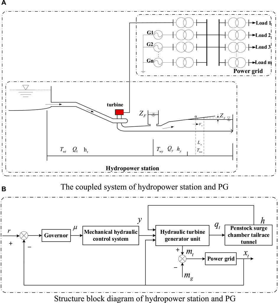
FIGURE 1. Coupled system and structure block diagram of the hydropower station and PG. (A) Coupled system of the hydropower station and PG. (B) Structure block diagram of the hydropower station and PG.

2.1 Mathematical model of the HTRS

As the actuator and core part of the HTRS, the governor which includes a controller and a servo system can balance the active power of power systems by adjusting the active power output from hydropower stations. The controller model applied in this paper is a parallel PI control structure, which can be represented as follows:

$\frac{dy}{dt}=-K_p\frac{d{x}_t}{dt}-K_i{x}_t,(1)$

where y is the output signal of the HURS governor; x_t is the relative deviation of the speed; and K_p and K_i represent the proportional gain and the integral gain, respectively.

The rigid model and elastic water hammer model are often utilized for a mathematical model of the pressure pipeline. For hydropower stations with long pressure pipelines, the elastic water hammer model is preferable to describe the characteristics of water flow in the pipe. However, as to hydropower stations with short pressure pipelines, it can be simplified to the rigid model. In this paper, the non-linear characteristics of flow and head loss are considered to establish the dynamic equation of the elastic water hammer model of the pressure pipeline (Liu and Guo, 2021).

$\frac{d{q}_t}{dt}=\frac{-h-Z_F-\frac{2h_t{q}_t}{H_0}}{T_{wt}},(2)$

where q_t is the flow rate of the pressure pipe; h is the relative deviation of the water head; Z_F is the water level of the downstream surge chamber; h_t is the head loss; H₀ is the initial water head; and T_wt is the inertial time constant of the water flow.

The dynamic equation of the downstream surge chamber is (Chaudhry, 2014)

$\frac{d{Z}_F}{dt}=\frac{q_t-q_y}{T_F},(3)$

where Z is the water level change of the downstream surge chamber; gr represents the flow rate of the diversion tunnel; gy is the flow rate of the tailrace tunnel; TF is the time constant of the downstream surge chamber; and T_F is a time constant of the surge chamber, $T_F=\frac{F{H}_0}{Q_{y0}}$.

The dynamic equation of the sloping roof tailrace tunnel is (Chaudhry, 2014)

$\frac{d{q}_y}{dt}=\frac{Z_F-\frac{2h_y{q}_y}{H_0}-z_y}{T_{wy}+T_{wx}}.(4)$

According to the work of Guo et al. (2015), T_wx and z_y are derived from Eqs 5, 6, respectively, and then, the dynamic equations of the sloping roof tailrace tunnel can be obtained by substituting Eqs 5, 6 into Eq. 4 as shown in Eq. 7.

$T_{wx}=\frac{\lambda Q_{y0}{V}_x{q}_y}{g{H}_{0}cW\tan \alpha },(5)$

$z_y=\frac{\lambda Q_{y0}{q}_y}{H_{0}cW},(6)$

$\frac{d{q}_y}{dt}=\frac{\frac{-2h_y{q}_y}{H_0}+Z_F-\frac{q_y{Q}_{y0}\lambda }{H_{0}cW}}{T_{wy}+\frac{q_y{Q}_{y0}\lambda V_x\cot \alpha }{g{H}_{0}cW}},(7)$

where h_y is the water head loss of the tailrace tunnel; z_y is the water level change of the tailrace tunnel; T_wy and T_wx represent the time constant of steady-state flow inertia and transient flow inertia, respectively; λ is the section coefficient of the tailrace tunnel; c is the wave velocity at the interface of the open and full-flow manifolds; W is the width of the tailrace tunnel; V_x is the flow rate at the open and full-flow interfaces; and α is the inclination angle of the tailrace tunnel.

The moment equation and flow equation of the hydraulic turbine are (Yang et al., 2019b)

$\begin{array}{c}{m}_t=e_x{x}_t+e_{y}y+e_{h}h,\\ q_t=e_{qx}{x}_t+e_{qy}y+e_{qh}h.\end{array}(8)$

In previous research, the first-order model of a synchronous generator was commonly employed to describe its inertia moment. Given the strong mechanical inertia of the hydraulic relay and water guide system, when the load changes, it is hard for the actuators to track and adjust quickly in real time, which leads to a lag phenomenon (Ma et al., 2021). To better reveal the dynamic characteristics of the HTRS coupled with the PG, this paper employs a second-order model of the synchronous generator, which depicts not only the rotational inertia but also the interaction between the electromagnetic power and the power angle. The mathematical model of synchronous generator is as follows:

$\frac{d{x}_t}{dt}=\frac{m_t-\left(e_g{x}_t+K_a\int \left(x_t-x_s\right)dt+D_a\left(x_t-x_s\right)+m_g\right)}{T_a}.(9)$

Since there is an integral term in Eq. 9, the state variable ξ₁ is defined as ${\xi }_1=\int \left(x_t-x_s\right)dt$. Equation 9 can be transformed into

$\begin{array}{c}\frac{d{\xi }_1}{dt}=x_t-x_s\\ \frac{d{x}_t}{dt}=\frac{m_t-\left(e_g{x}_t+K_a{\xi }_1+D_a\left(x_t-x_s\right)+m_g\right)}{T_a},\end{array}(10)$

where ξ₁ is the intermediate state variable; x_s is the relative deviation value of the grid frequency; e_g is the self-regulation coefficient of the load; K_a is the equivalent synchronization coefficient; D_a is the equivalent damping coefficient; m_g is the relative deviation of the resistance torque; and T_a is the inertial time constant of the unit.

2.2 Mathematical model of the PG

The structural block diagram of the equivalent PG is shown in Figure 2. Load disturbance only considers mg, ignoring load disturbance in the PG, i.e., p_l = 0. The dynamic equations of the equivalent PG can be deduced from Figure 2 as shown in the following (Guo and Peng, 2020):

$\begin{array}{c}\frac{d{\xi }_2}{dt}=x_s-\frac{{\xi }_2}{T_g},\\ \frac{d{x}_s}{dt}=\frac{B{p}_t-D_s{x}_s-\frac{{\xi }_2}{T_g{R}_g}}{T_s},\end{array}(11)$

where ξ₂ is the intermediate state variable; T_g is the inertia time constant of the servo motor in the grid model; B is the power conversion coefficient; p_t is the power output; D_s is the self-regulation coefficient of the equivalent load; difference coefficient; and R_g is the inertia time constant of the grid equivalent unit.

FIGURE 2

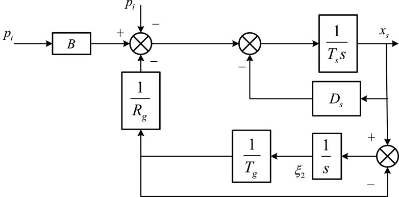
FIGURE 2. Structural block diagram of the equivalent PG.

By integrating Eqs 1–4 and Eqs 9–11, the eighth-order non-linear state equations are obtained as Eq. 12, which can reflect the coupling effect of the HTRS and PG.

$\left\{\begin{array}{c}\frac{d{x}_t}{dt}=\frac{1}{T_a}\left[-m_g-e_g{x}_t+e_x{x}_t-D_a\left(x_t-x_s\right)+e_{y}y+\frac{e_h}{e_{qh}}\left(q_t-e_{qx}{x}_t-e_{qy}y\right)-K_a{\xi }_1\right]\\ \frac{dy}{dt}=-K_i{x}_t-\frac{K_p}{T_a}\left[-m_g-e_g{x}_t+e_x{x}_t-D_a\left(x_t-x_s\right)+e_{y}y+\frac{e_h}{e_{qh}}\left(q_t-e_{qx}{x}_t-e_{qv}y\right)-K_a\xi \right]\\ \frac{d{\xi }_1}{dt}=x_t-x_s\\ \frac{d{x}_s}{dt}=\frac{1}{T_s}\left[-\left(D_s-B{D}_a\right)x_s+B{D}_a{x}_t+B{K}_a{\xi }_1-\frac{{\xi }_2}{R_g{T}_g}\right]\\ \frac{d{\xi }_2}{dt}=x_s-\frac{{\xi }_2}{T_g}\\ \frac{d{q}_t}{dt}=\frac{1}{T_{wt}}\left[\frac{-2h_t{q}_t}{H_0}-\frac{1}{e_{qh}}\left(q_t-e_{qx}{x}_t-e_{qv}y\right)-Z_F\right]\\ \frac{d{Z}_F}{dt}=\frac{1}{F{H}_0}\left(q_t-q_y\right)Q_{y0}\\ \frac{d{q}_y}{dt}=\frac{g\left(cW\left(-2h_y{q}_y+H_0{Z}_F\right)-q_y{Q}_{y0}\lambda \right)}{cg{H}_0{T}_{wy}W+q_y{Q}_{y0}{V}_x\lambda \cot \alpha }.\end{array}\right.(12)$

3 Stability of the non-linear HTRS

3.1 Stability analysis method

Hopf bifurcation (Strogatz, 2014; Wiggins, 2013) is a simple yet important dynamic bifurcation phenomenon in non-linear systems, which is a type of localized dynamic bifurcation; specifically, as the bifurcation parameter varies, the system bifurcates abruptly from the equilibrium at the non-hyperbolic equilibrium from the extremal limit loop phenomenon. Accordingly, Hopf bifurcation theory with theoretical applicability, simple program design, and high calculation accuracy is generally applied to conduct non-linear analysis. Meanwhile, Hopf bifurcation theory has been applied to the dynamics research of the HTRS in relevant works. Thus, this theory can be adopted in this paper to investigate the non-linear dynamical behavior of the coupled system.

Under external perturbations, the system will generate steady-state or unsteady-state limit-loop oscillations at Hopf bifurcation points, which correspond to supercritical and subcritical bifurcations, respectively. The Jacobian matrix of the coupled system at the equilibrium point X_E is J(μ) = Df_x(X_E,μ). Accordingly, the characteristic equation of the Jacobian matrix can be derived by det(J(μ) - λI) = 0 as follows:

${\lambda }^n+a_1{\lambda }^{n-1}+a_2{\lambda }^{n-2}+\cdots +a_{n-1}\lambda +a_n=0,(13)$

where λ and a_i(μ) (i = 1,2, ,n) are eigenvalues and coefficients of the polynomial det(J(μ) - λI) = 0, respectively.

The existence of Hopf bifurcation can be validated by the following well-known Hurwitz criterion (Hassard et al., 1981):

$a_i>0\left(i=\mathrm{1,2},\cdots ,n\right),(14)$

${\Delta }_2=\det \left[\begin{array}{cc}{a}_1& 1\\ a_3& a_2\end{array}\right]>0,(15)$

${\Delta }_3=\det \left[\begin{array}{ccc}{a}_1& 1& 0\\ a_3& a_2& a_1\\ a_5& a_4& a_3\end{array}\right]>0,(16)$

${\Delta }_7=\det \left[\begin{array}{ccccccc}{a}_1& 1& 0& 0& 0& 0& 0\\ a_3& a_2& a_1& 1& 0& 0& 0\\ a_5& a_4& a_3& a_2& a_1& 0& 0\\ a_7& a_6& a_5& a_4& a_3& a_2& a_1\\ 0& a_8& a_7& a_6& a_5& a_4& a_3\\ 0& 0& 0& a_8& a_7& a_6& a_5\\ 0& 0& 0& 0& 0& a_8& a_7\end{array}\right]=0.(17)$

If Eqs 14–17 are satisfied at μ = μ_c, Eq. 13 has a pair of pure virtual eigenvalues λ_1,2 = ±iω_c and the system will bifurcate at μ = μ_c. Accordingly, the system will occur with periodic oscillations and generate limit cycles in phase space. The limit cycle period at Hopf bifurcation is T_LC = 2π∕ω_c. Furthermore, the type of Hopf bifurcation can be determined based on the cross-sectional coefficient ${\sigma }^{\prime }\left({\mu }_c\right)=\text{Re}\left({\left.\frac{\mathrm{d}\lambda }{\mathrm{d}\mu }\right|}_{\mu ={\mu }_c}\right)$.

3.2 Stability analysis of the HTRS and PG

According to Eq. 12, variables x_t, y, ξ₁, x_s, ξ₂, q_t, Z_F, and q_y are chosen as state variables of the coupled system, and state vector X = (x_t, y, ξ₁, x_s, ξ₂, q_t, Z_F, q_y)^T can be obtained. With the exception of state variables, any other parameter in Eq. 12 can be chosen as the bifurcation parameter, denoted as μ. The choice of bifurcation parameter μ is based on the purpose of system research. For example, K_p and K_i are chosen as bifurcation parameters when studying the effect of the governor on the stability of the whole system.

The equilibrium point X_E = (x_tE, y_E, ξ_1E, x_sE, ξ_2E, q_tE, Z_FE, q_yE)^T can be obtained by solving f(x, μ) = 0, i.e., by making Eq. 12 = 0:

$\left\{\begin{array}{l}{x}_{tE}=0\\ y_E=\frac{m_g\left(c\left(H_0+2e_{qh}\left(h_t+h_y\right)\right)W+e_{qh}{Q}_{y0}\lambda \right)}{c\left(-2e_h{e}_{qy}\left(h_t+h_y\right)+e_y\left(H_0+2e_{qh}\left(h_t+h_y\right)\right)\right)W+\left(-e_h{e}_{qy}+e_{qh}{e}_y\right)Q_{y0}\lambda }\\ {\xi }_{1E}=0\\ x_{sE}=0\\ {\xi }_{2E}=0\\ q_{tE}=-\frac{c{e}_{qv}{H}_0{m}_{g}W}{2c{e}_h{e}_{qy}\left(h_t+h_y\right)W-c{e}_y\left(H_0+2e_{qh}\left(h_t+h_y\right)\right)W+\left(e_h{e}_{qy}-e_{qh}{e}_y\right)Q_{y0}\lambda }\\ Z_{FE}=-\frac{e_{qy}{m}_g\left(2c{h}_{y}W+Q_{y0}\lambda \right)}{2c{e}_h{e}_{qy}\left(h_t+h_y\right)W-c{e}_y\left(H_0+2e_{qh}\left(h_t+h_y\right)\right)W+\left(e_h{e}_{qy}-e_{qh}{e}_y\right)Q_{y0}\lambda }\\ q_{yE}=-\frac{c{e}_{qy}{H}_0{m}_{g}W}{2c{e}_h{e}_{qy}\left(h_t+h_y\right)W-c{e}_y\left(H_0+2e_{qh}\left(h_t+h_y\right)\right)W+\left(e_h{e}_{qy}-e_{qh}{e}_y\right)Q_{y0}\lambda .}\end{array}\right.(18)$

The Jacobian matrix J(μ) for solving the non-linear coupled system $\dot{x}=f\left(x,\mu \right)$ is

$J\left(\mu \right)=D{f}_x\left(x,\mu \right)=\left[\begin{array}{cccccccc}\frac{\partial {\dot{x}}_t}{\partial x_t}& \frac{\partial {\dot{x}}_t}{\partial y}& \frac{\partial {\dot{x}}_t}{\partial {\xi }_1}& \frac{\partial {\dot{x}}_t}{\partial x_s}& \frac{\partial {\dot{x}}_t}{\partial {\xi }_2}& \frac{\partial {\dot{x}}_t}{\partial q_t}& \frac{\partial {\dot{x}}_t}{\partial Z_F}& \frac{\partial {\dot{x}}_t}{\partial q_y}\\ \frac{\partial \dot{y}}{\partial x_t}& \frac{\partial \dot{y}}{\partial y}& \frac{\partial \dot{y}}{\partial {\xi }_1}& \frac{\partial \dot{y}}{\partial x_s}& \frac{\partial \dot{y}}{\partial {\xi }_2}& \frac{\partial \dot{y}}{\partial q_t}& \frac{\partial \dot{y}}{\partial Z_F}& \frac{\partial \dot{y}}{\partial q_y}\\ \frac{\partial {\dot{\xi }}_1}{\partial x_t}& \frac{\partial {\dot{\xi }}_1}{\partial y}& \frac{\partial {\dot{\xi }}_1}{\partial {\xi }_1}& \frac{\partial {\dot{\xi }}_1}{\partial x_s}& \frac{\partial {\dot{\xi }}_1}{\partial {\xi }_2}& \frac{\partial {\dot{\xi }}_1}{\partial q_t}& \frac{\partial {\dot{\xi }}_1}{\partial Z_F}& \frac{\partial {\dot{\xi }}_1}{\partial q_y}\\ \frac{\partial {\dot{x}}_s}{\partial x_t}& \frac{\partial {\dot{x}}_s}{\partial y}& \frac{\partial {\dot{x}}_s}{\partial {\xi }_1}& \frac{\partial {\dot{x}}_s}{\partial x_s}& \frac{\partial {\dot{x}}_s}{\partial {\xi }_2}& \frac{\partial {\dot{x}}_s}{\partial q_t}& \frac{\partial {\dot{x}}_s}{\partial Z_F}& \frac{\partial {\dot{x}}_s}{\partial q_y}\\ \frac{\partial {\dot{\xi }}_2}{\partial x_t}& \frac{\partial {\dot{\xi }}_2}{\partial y}& \frac{\partial {\dot{\xi }}_2}{\partial {\xi }_1}& \frac{\partial {\dot{\xi }}_2}{\partial x_s}& \frac{\partial {\dot{\xi }}_2}{\partial {\xi }_2}& \frac{\partial {\dot{\xi }}_2}{\partial q_t}& \frac{\partial {\dot{\xi }}_2}{\partial Z_F}& \frac{\partial {\dot{\xi }}_2}{\partial q_y}\\ \frac{\partial {\dot{q}}_t}{\partial x_t}& \frac{\partial {\dot{q}}_t}{\partial y}& \frac{\partial {\dot{q}}_t}{\partial {\xi }_1}& \frac{\partial {\dot{q}}_t}{\partial x_s}& \frac{\partial {\dot{q}}_t}{\partial {\xi }_2}& \frac{\partial {\dot{q}}_t}{\partial q_t}& \frac{\partial {\dot{q}}_t}{\partial Z_F}& \frac{\partial {\dot{q}}_t}{\partial q_y}\\ \frac{\partial {\dot{Z}}_F}{\partial x_t}& \frac{\partial {\dot{Z}}_F}{\partial y}& \frac{\partial {\dot{Z}}_F}{\partial {\xi }_1}& \frac{\partial {\dot{Z}}_F}{\partial x_s}& \frac{\partial {\dot{Z}}_F}{\partial {\xi }_2}& \frac{\partial {\dot{Z}}_F}{\partial q_t}& \frac{\partial {\dot{Z}}_F}{\partial Z_F}& \frac{\partial {\dot{Z}}_F}{\partial q_y}\\ \frac{\partial {\dot{q}}_y}{\partial x_t}& \frac{\partial {\dot{q}}_y}{\partial y}& \frac{\partial {\dot{q}}_y}{\partial {\xi }_1}& \frac{\partial {\dot{q}}_y}{\partial x_s}& \frac{\partial {\dot{q}}_y}{\partial {\xi }_2}& \frac{\partial {\dot{q}}_y}{\partial q_t}& \frac{\partial {\dot{q}}_y}{\partial Z_F}& \frac{\partial {\dot{q}}_y}{\partial q_y}\end{array}\right],(19)$

where $\begin{array}{c}\frac{\partial {\dot{x}}_t}{\partial x_t}=\frac{-D_a-e_y-\frac{e_h{e}_{qx}}{e_{qh}}+e_x}{T_a},\frac{\partial {\dot{x}}_t}{\partial y}=\frac{\frac{-e_h{e}_{qy}}{e_{qh}}+e_y}{T_a},\frac{\partial {\dot{x}}_t}{\partial {\xi }_1}=\frac{-K_a}{T_a},\frac{\partial {\dot{x}}_t}{\partial x_s}=\frac{D_a}{T_a},\frac{\partial {\dot{x}}_t}{\partial {\xi }_2}=0,\\ \frac{\partial {\dot{x}}_t}{\partial q_t}=\frac{e_h}{e_{qh}{T}_a},\frac{\partial {\dot{x}}_t}{\partial Z_F}=0,\frac{\partial {\dot{x}}_t}{\partial q_y}=0,\frac{\partial \dot{y}}{\partial x_t}=\frac{e_h{e}_{qx}{K}_p+e_{qh}\left(D_a+e_g-e_x\right)K_p-e_{qh}{K}_i{T}_a}{e_{qh}{T}_a},\frac{\partial \dot{y}}{\partial y}=\frac{e_h{e}_{qy}{K}_p-e_{qh}{e}_y{K}_p}{e_{qh}{T}_a},\frac{\partial \dot{y}}{\partial {\xi }_1}=\frac{K_a{K}_p}{T_a},\frac{\partial \dot{y}}{\partial x_s}\\ =-\frac{D_a{K}_p}{T_a},\frac{\partial \dot{y}}{\partial {\xi }_2}=0,\frac{\partial \dot{y}}{\partial q_t}=-\frac{e_h{K}_p}{e_{qh}{T}_a},\frac{\partial \dot{y}}{\partial Z_F}=0,\frac{\partial \dot{y}}{\partial q_y}=0,\frac{\partial {\dot{\xi }}_1}{\partial x_t}=1,\frac{\partial {\dot{\xi }}_1}{\partial y}=0,\frac{\partial {\dot{\xi }}_1}{\partial {\xi }_1}\\ =0,\frac{\partial {\dot{\xi }}_1}{\partial x_s}=-1,\frac{\partial {\dot{\xi }}_1}{\partial {\xi }_2}=0,\frac{\partial {\dot{\xi }}_1}{\partial q_t}=0,\frac{\partial {\dot{\xi }}_1}{\partial Z_F}=0,\frac{\partial {\dot{\xi }}_1}{\partial q_y}=0,\frac{\partial {\dot{x}}_s}{\partial x_t}=\frac{B{D}_a}{T_s},\frac{\partial {\dot{x}}_s}{\partial y}=0,\frac{\partial {\dot{x}}_s}{\partial {\xi }_1}=\frac{B{K}_a}{T_s},\frac{\partial {\dot{x}}_s}{\partial x_s}=\frac{B{D}_a-D_s}{T_s},\\ \frac{\partial {\dot{x}}_s}{\partial {\xi }_2}=-\frac{1}{R_g{T}_g{T}_s},\frac{\partial {\dot{x}}_s}{\partial q_t}=0,\frac{\partial {\dot{x}}_s}{\partial Z_F}=0,\frac{\partial {\dot{x}}_s}{\partial q_y}=0,\frac{\partial {\dot{\xi }}_2}{\partial x_t}=0,\frac{\partial {\dot{\xi }}_2}{\partial y}=0,\frac{\partial {\dot{\xi }}_2}{\partial {\xi }_1}=0,\frac{\partial {\dot{\xi }}_2}{\partial x_s}=1,\frac{\partial {\dot{\xi }}_2}{\partial {\xi }_2}=-\frac{1}{T_g},\frac{\partial {\dot{\xi }}_2}{\partial q_t}=0,\frac{\partial {\dot{\xi }}_2}{\partial Z_F}=0,\frac{\partial {\dot{\xi }}_2}{\partial q_y}=0,\\ \frac{\partial {\dot{q}}_t}{\partial x_t}=\frac{e_{qx}}{e_{qh}{T}_{wt}},\frac{\partial {\dot{q}}_t}{\partial y}=\frac{e_{qy}}{e_{qh}{T}_{wt}},\frac{\partial {\dot{q}}_t}{\partial {\xi }_1}=0,\frac{\partial {\dot{q}}_t}{\partial x_s}=0,\frac{\partial {\dot{q}}_t}{\partial {\xi }_2}=0,\frac{\partial {\dot{q}}_t}{\partial q_t}=\frac{1}{T_{wt}}\left(\frac{-1}{e_{qh}}-\frac{2h_t}{H_0}\right),\frac{\partial {\dot{q}}_t}{\partial Z_F}=-\frac{1}{T_{wt}},\frac{\partial {\dot{q}}_t}{\partial q_y}=0,\\ \frac{\partial {\dot{Z}}_F}{\partial x_t}=0,\frac{\partial {\dot{Z}}_F}{\partial y}=0,\frac{\partial {\dot{Z}}_F}{\partial {\xi }_1}=0,\frac{\partial {\dot{Z}}_F}{\partial x_s}=0,\frac{\partial {\dot{Z}}_F}{\partial {\xi }_2}=0,\frac{\partial {\dot{Z}}_F}{\partial q_t}=\frac{Q_{y0}}{F{H}_0},\frac{\partial {\dot{Z}}_F}{\partial Z_F}=0,\frac{\partial {\dot{Z}}_F}{\partial q_y}=-\frac{Q_{y0}}{F{H}_0},\frac{\partial {\dot{q}}_y}{\partial x_t}=0,\frac{\partial {\dot{q}}_y}{\partial y}=0,\\ \frac{\partial {\dot{q}}_y}{\partial {\xi }_1}=0,\frac{\partial {\dot{q}}_y}{\partial x_s}=0,\frac{\partial {\dot{q}}_y}{\partial {\xi }_2}=0,\frac{\partial {\dot{q}}_y}{\partial q_t}=0,\frac{\partial {\dot{q}}_y}{\partial Z_F}=\frac{cg{H}_{0}W}{cg{H}_0{T}_{wy}W+q_y{Q}_{y0}{V}_x\lambda \cot \alpha },\frac{\partial {\dot{q}}_y}{\partial q_y}=-\frac{g{Q}_{y0}{V}_x\lambda \left(cW\left(-2h_y{q}_y+H_0{Z}_F\right)-q_y{Q}_{y0}\lambda \right)\cot \alpha }{{\left(cg{H}_0{T}_{wy}W+q_y{Q}_{y0}{V}_x\lambda \cot \alpha \right)}^2}+\frac{g\left(-2c{h}_{y}W-Q_{y0}\lambda \right)}{cg{H}_0{T}_{wy}W+q_y{Q}_{y0}{V}_x\lambda \cot \alpha }\end{array}$.

The characteristic polynomial of the Jacobian matrix J(μ) is

$x^8+a_1{x}^7+a_2{x}^6+a_3{x}^5+a_4{x}^4+a_5{x}^3+a_6{x}^2+a_{7}x+a_8=0.(20)$

Based on the aforementioned stability analysis criterion, the stability domain can be drawn on the K_p–K_i plane. Parameter values of the HTRS and PG are T_a = 10 s, T_wt = 3.5 s, F = 1,500 m², T_wy = 2.0 s, W = 7.5 m, m_g = −0.1, e_g = 0, e_x = −1, e_y = 1, e_h = 1.5, h_t = 1.46 m, H₀ = 80 m, e_qx = 0, e_qy = 1, e_qh = 0.5, h_y = 1.12 m, Q_y0 = 500 m³/s, H_x = 18.3 m, α = 0.0599282, D_a = 0.073, K_a = 2, T_s = 40, D_s = 0.4, R_g = 0.2, T_g = 40, and B = 0.1, and x denotes the eigenvalue of the polynomial J(μ) with value 3.

The bifurcation line is a crucial stability indicator comprising all Hopf bifurcation points on the K_p–K_i plane, which divides the whole parameter plane into stable and unstable domains. Thus, the location of bifurcation line determines stability margin in the parameter plane of the coupled system that also reflects dynamic characteristics.

With respect to the non-linear coupled system researched in this paper, K_i is chosen as the bifurcation parameter. Then, the stable domain and bifurcation line of the coupled system can be determined by solving Eq. 12, and they are shown in Figure 3A. In Figure 3A, three state points s₁, s₂, and s₃ are chosen to investigate dynamic response of the coupled system under different parameter values. Coordinate values of the three selected state points and respective theoretical states of the dynamic response are shown in Table 1. In addition, from Figure 3B, it can be concluded that σ'(μ_c) > 0, which indicates that the Hopf bifurcation is supercritical.

FIGURE 3

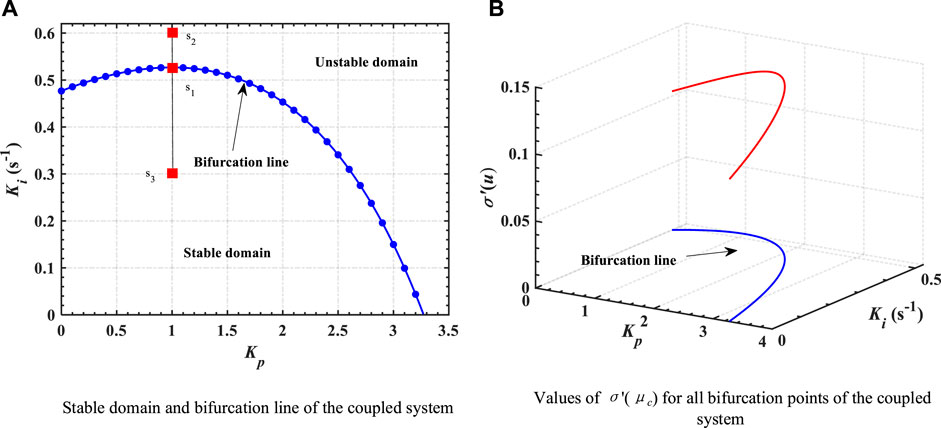
FIGURE 3. Non-linear dynamics of the coupled system. (A) Stable domain and bifurcation line of the coupled system. (B) Values of σ'(μ_c) bifurcation points of the coupled system.

TABLE 1

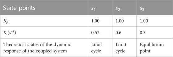
TABLE 1. Coordinate values of s₁, s₂, and s₃.

3.3 Numerical analysis and stability verification

According to chaos theory and Hopf bifurcation theory, the discriminant conditions for Hopf bifurcation to occur in the system are Eqs 14–17. With the aim of verifying the correctness of the conclusions in Table 1, numerical simulation experiments are utilized in this section. Three state points s₁, s₂, and s₃ are substituted into the state equation to solve the dynamic response of system state variables. Dynamic characteristics and the phase space trajectory of the state variables for the three corresponding state points are shown in Figure 4. The equilibrium point of the system is often chosen as the initial state of the system when simulation experiments of non-linear systems are carried out. Therefore, all the parameters of the system are substituted into the system of state equations and the equilibrium point of the state variables of the system is solved, and the state of the equilibrium point is obtained to be (−0.1335, 0). So, (−0.1335, 0) is chosen to be the initial state of the system.

FIGURE 4

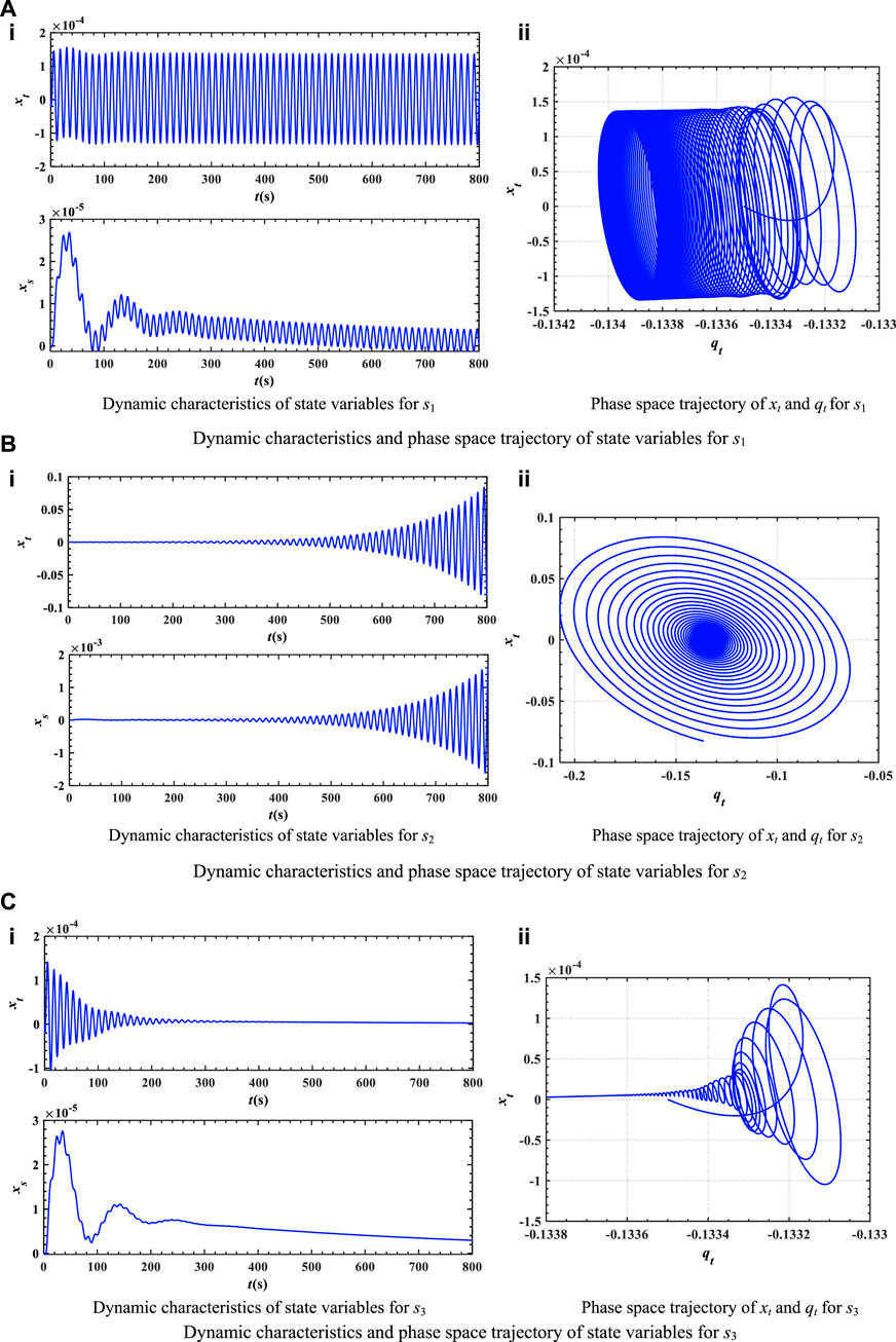
FIGURE 4. Dynamic characteristics and phase space trajectory of state variables. (A) Dynamic characteristics and phase space trajectory of state variables for s₁. (B) Dynamic characteristics and phase space trajectory of state variables for s₂. (C) Dynamic characteristics and phase space trajectory of state variables for s₃.

The conclusions that can be obtained from Figure 4 are as follows:

(1) Figure 4A shows that Hopf bifurcation occurs at s₁, which is coherent with the aforementioned theoretical analysis. From the phase space trajectory in Figure 4A, it can be concluded that at point s₁, the system oscillates from the equilibrium point and quickly enters limit cycles. Furthermore, when the load disturbance of the coupled system is m_g = −0.1, state variables x_s and x_t oscillate with equal amplitude from the equilibrium point.

(2) From Figure 3, it can be seen that the s₂ point is in an unstable domain and bifurcation parameters are K_p = 1 and K_i = 0.6. According to the phase space trajectory of x_t and q_t in Figure 4B, it can also be shown that the state of point s₂ is unstable, and the trajectory of state variables gradually diverges from the equilibrium point. In addition, from dynamic characteristics of each state variable, it can also be concluded that point s₂ is unstable, which will lead to gradual instability of the system operation.

(3) Figure 4C investigates dynamic characteristics of point s₃ when bifurcation parameters are K_p = 1 and K_i = 0.3. From Figure 4C, it can be known that state variables begin to converge gradually from the equilibrium point. Moreover, from dynamic characteristics of state variables, it can be concluded that as time increases, the oscillation amplitude of each variable gradually decreases and finally becomes stable.

4 Coupling effect of the HTRS and PG

4.1 Influence of dynamic performance

The highly complex dynamic behavior and significant impact on the stability region are consequences of the complex non-linear characteristics inherent to the HTRS. In order to reveal the coupling effect between the HTRS and PG, the coupled system was partitioned into two subsystems for non-linear dynamics analysis. This type of analysis enables a deeper understanding of the dynamic characteristics of the HTRS and PG, revealing the interrelationship between them and allowing for a more precise evaluation of system stability.

Subsystem 1 is the hydropower station considering a downstream surge chamber and sloping roof tailrace tunnel, while subsystem 2 is the PG. For subsystem 1, since the downstream surge chamber and sloping roof tailrace tunnel can decrease water hammer pressure during the transition process of the hydropower station, the influence of the downstream surge chamber and sloping roof tailrace tunnel on the operation of the hydropower station has to be considered. Although the tailrace tunnel can reduce the loss of outlet kinetic energy by using a turbine runner, water level fluctuation of the surge chamber and flow inertia variation of the tailrace tunnel will also interfere with the system. Moreover, the disturbance interaction not only directly affects stability of the hydropower station but also generates complex dynamic behavior during transients. Due to the fact that subsystem 2 is directly coupled to the hydropower station, changes of PG load and the connection and exit of power will affect safe operation of the coupled system. Hence, it is essential to study subsystem 1 and subsystem 2 on the dynamic behavior and stability of the coupled system.

4.1.1 Influence of the HTRS on stable domain and dynamic characteristics

This section studies the dynamic behavior and stability of the HTRS. With the state equation of the HTRS, the influence factors of dynamic characteristics are analyzed by drawing stability domain and dynamic response under different characteristic parameters. Parameters F, T_a, T_wt, and T_wy are selected as characteristic parameters of the coupled system under load disturbance m_g = −0.1. Then, within a reasonable range, different values of F, T_a, T_wt, and T_wy are selected, whose corresponding parameter values are shown in Table 2. To assist analysis, four state points are selected and the stability domain and dynamic response are analyzed under different characteristic parameters.

TABLE 2

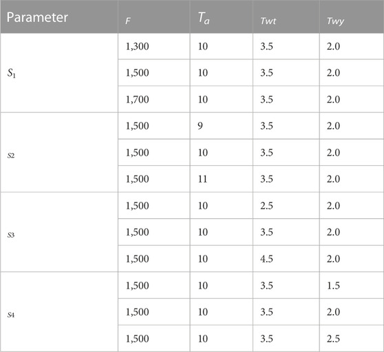
TABLE 2. Parameter values of characteristic parameters.

The impact of characteristic parameters on the stability domain is demonstrated in Figure 5. Through the analysis of the stability domain and bifurcation line, the following conclusions can be obtained.

FIGURE 5

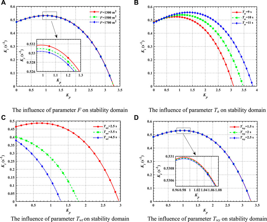
FIGURE 5. Influence of characteristic parameters on the stability domain. (A) The influence of parameter F on stability domain. (B) The influence of parameter T_a on stability domain. (C) The influence of parameter T_wt on stability domain. (D) The influence of parameter T_wy on stability domain.

The horizontal and vertical coordinates of the stability region and bifurcation line are K_p and K_i, respectively. According to Figure 5A, F is set as 1,300; 1,500; and 1,700 m², respectively. Figure 5A shows a slight influence of F on the stability domain of the system. As F increases, the bifurcation line of stable domains of the coupled system moves toward a lower-left corner of the K_p–K_i plane, indicating that stability is better for smaller F. Hence, adopting a smaller F value can improve the system’s stability domain. Nonetheless, it should be noted that the improvement achieved by adjusting F is limited and F cannot be regarded as the primary factor for enhancing the stability of the coupled system.

According to Figures 5B, C, T_a is set as 9, 10, and 11 s. T_wt is set as 2.5, 3.5, and 4.5 s. Figures 5B, C show a significant effect of T_a and T_wt on the stability domain of the system. An intersection of bifurcation lines of the stability domain exists with different T_a. To the left side of the intersection point, the stability domain decreases as T_a increases. However, on the right side of the intersection point, the change in the stable domain behaves oppositely. With the increase of T_wt, the bifurcation line of the stability domain of the system moves to the down left corner of the K_p–K_i plane, indicating that a smaller T_wt results in better stability. Hence, T_a can improve the system stability by determining appropriate T_a value based on the intersection point. In addition, to enhance system stability, a smaller T_wt value is recommended. In practical applications, adopting a smaller T_wt value is a feasible measure to improve the system stability.

From Figure 5D, T_wy is set as 1.5, 2, and 2.5 s. Figure 5D shows a slight effect of T_wy on the stability domain of the coupled system. As T_wy increases, the bifurcation line of the stability domain is shifted toward the bottom left angle of the K_p–K_i plane, indicating that a smaller T_wy results in better stability. Therefore, for the purpose of enhancing system stability, a smaller T_wy value may be advisable. However, enhancement extent is small and the T_wy value cannot be taken as the major method to improve the stability of the coupled system.

By numerical simulation, the influence of four parameters on dynamic characteristics can be derived, whose results are shown in Figure 6.

FIGURE 6

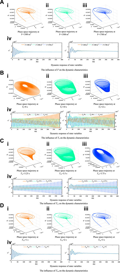
FIGURE 6. Influence on the dynamic characteristics. (A) The influence of F on the dynamic characteristics. (B) The influence of T_a on the dynamic characteristics. (C) The influence of T_wt on the dynamic characteristics. (D) The influence of T_wy on the dynamic characteristics.

According to the phase space trajectory in Figures 6Ai–iii, under different values of parameter F, state variables gradually decay to the equilibrium point. Furthermore, from Figure 6Aiv, it can be observed that the effect of F on the dynamic response of state variables is very slight, and it has almost no effect on the head wave crest of state variables. The values and appearance times of wave crests are almost the same when F values are different. The results show that F has almost no effect on dynamic performance.

The influence of T_a on the dynamic characteristics at load disturbance m_g = −0.1, T_a = 8 s, T_a = 10 s, and T_a = 12 s is shown in Figure 6B. By observing phase space trajectories of state variables in Figures 6Bi–iii, it can be seen that when parameter T_a = 8 s, the phase space trajectory presents divergent motion; when T_a = 10 s, Hopf bifurcation occurs and limit cycles are generated; however, at T_a = 12 s, the phase space trajectory gradually converges. In Figure 6Biv, T_a has almost no effect on the head wave of state variables but has an enormous effect on the tail wave. Specifically, with larger T_a, tail wave fluctuations become smoother, indicating that the system is easier to stabilize, whereas the opposite is true for smaller T_a.

The influence of T_wt on the dynamic characteristics at T_wt = 3.25 s, T_wt = 3.5 s, and T_wt = 3.75 s is shown in Figure 6C. From the dynamic response and phase space trajectory of state variables in Figure 6C, it can be seen that state variables undergo divergent, convergent, and equal amplitude oscillatory motion for different values of T_wt. It is shown that T_wt has a very significant impact on the stability and dynamic performance of the coupled system. By observing Figure 6Civ, it becomes evident that parameter T_wt can change the operating status and stability, which can be considered a primary measure to regulate the dynamic property of the coupled system.

Figure 6D studies the influence of T_wy on the dynamic characteristics. At different T_wy values, T_wy has little effect on the dynamic characteristics of state variables. Moreover, the trends of state variables are almost the same. To sum up, T_wy has little influence on dynamic performance and generally does not change the running state of the coupled system.

4.1.2 Influence of the PG on stable domain and dynamic characteristics

To investigate the influence of the PG on the stable domain and dynamic properties of the system, stability region, power spectrum, and dynamic response under different B, D_s, T_s, R_g, and T_g are drawn and the results are shown in Figure 7. The specific PG parameter values are given in Table 3.

FIGURE 7

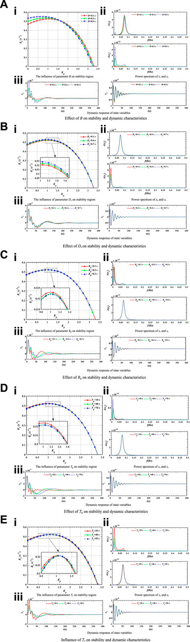
FIGURE 7. Influence of each state variables on stability and dynamic characteristics. (A) Effect of B on stability and dynamic characteristics. (B) Effect of D_s on stability and dynamic characteristics. (C) Effect of R_g on stability and dynamic characteristics. (D) Effect of T_g on stability and dynamic characteristics. (E) Influence of Ts on stability and dynamic characteristics.

TABLE 3

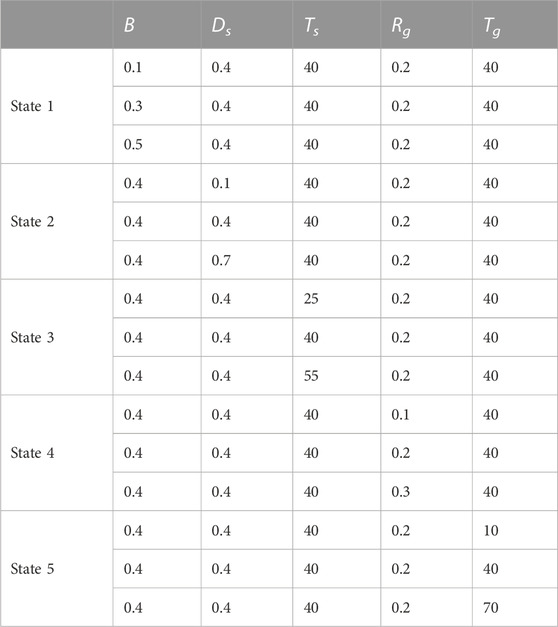
TABLE 3. Specific PG parameter values.

Figure 7A illustrates the significant influence of B on the stability region, power spectrum, and dynamic response of the coupled system. For different values of B, the bifurcation line demonstrates an intersection point. On the left side of this intersection, the stability domain increases with the rise of B. Conversely, on the right side, the stability domain exhibits a contrary change rate. Figure 7Aii illustrates that there are two wave peaks in the power spectrum of x_s and that B has the same effect on the two wave peaks. Furthermore, the amplitude of two subwaves in the x_s power spectrum becomes larger as B increases. The influence of B on the power spectrum of x_t is relatively small, but the effect on the two wave peaks is opposite. The dynamic response of state variables is illustrated in Figure 7Aiii. B has a substantial impact on the head wave and a smaller effect on the tail wave. Thus, B can improve system stability, while not improving the dynamic response of state variables.

Figure 7B shows the effect of D_s on stability and dynamic characteristics. According to Figure 7Bi, the stability region increases slightly with the increase of D_s, which indicates that D_s can improve the stability of the coupled system. According to the power spectrum of x_t and x_s, it can be found that the change of D_s has little effect on the power spectrum of x_t, but has a significant effect on x_s. With the increase of D_s, the amplitude of the 1st wave decreases, while period and frequency remain unvaried. From Figure 7Biii, it can be seen that D_s possesses no prominent effect on the dynamic response of x_t. In summary, as D_s increases, the convergence rate of x_s can be accelerated and the attenuation degree of the power spectrum of x_s can be improved.

It can be seen from Figure 7C that R_g has no significant influence on the stability region of the coupled system. According to Figure 7Cii, it can be concluded that R_g has a great influence on the power spectrum of x_s. The period of the 1st wave of x_s increases, and decay rate decreases when R_g becomes larger. However, for the 2nd wave, as R_g increases, the decay rate of x_s becomes larger slightly and the period remains unchanged. It can be obtained from Figure 7Ciii that R_g possesses a great effect on the dynamic response of x_s, which not only affects the amplitude of oscillation but also affects convergence time. In conclusion, the R_g impact on the stabilization domain and dynamic properties of the coupled system is not significant, so dynamic performance can hardly be enhanced with the adjustment of R_g.

Figure 7Di indicates that the stability domain corresponding to each T_g value is almost the same, so the effect of T_g on the stable domain of the coupled system is small. From Figure 7Dii, it can be obtained that T_g has almost no effect on the power spectrum of the state variable x_t, while its effect on x_s is obvious. Moreover, T_g not only affects amplitude but also the period of x_s. Accordingly, as T_g becomes larger, the period of the 1st wave of the power spectrum increases, while the attenuation rate reduces, but there exists almost no effect on the 2nd wave. From Figure 7Diii, it can also be found that with the increase of T_g, the regulation time of x_s is longer. Hence, the stability and dynamic properties of the coupled system cannot be appreciably enhanced with adjusting T_g.

It can be found from Figure 7Ei that T_s has a significant impact on the stability region. Specifically, under different T_s values, there is an intersection of the bifurcation line. On the left of the intersection, as T_s increases, the stability region increases. However, on the right of the intersection, the result is opposite. Figure 7Eii shows that T_s has little influence on x_t, but it has a greater influence on x_s and its effect on the amplitude and period of power spectrum. Correspondingly, as T_s increases, the amplitude and period of the power spectrum of x_s decrease. Thus, smaller T_s are recommended to improve stabilization and dynamic properties of the coupled system.

4.2 Eigenvalue analysis

The Jacobi matrix of the coupled system is obtained by differentiating state variables according to Eq. 12. According to matrix theory and Hopf bifurcation theory, a pair of purely imaginary eigenvalues will appear when Hopf bifurcation occurs, so this pair of eigenvalues is selected to analyze the stability of the coupled system, as shown in Figure 8.

FIGURE 8

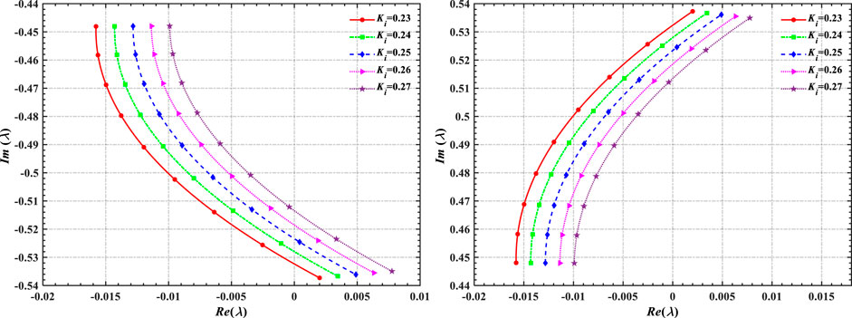
FIGURE 8. Variation law of eigenvalues of the Jacobi matrix with controller parameters.

Based on Figure 8, it can be concluded that two eigenvalues have the same change rule with controller parameters. When K_i is constant, with the increase of K_p, the real part of eigenvalue increases and the imaginary part decreases. The coupled system is unstable when the real part of eigenvalues is greater than zero, so it gradually transitions from the stable region to unstable region as K_p increases. Furthermore, as K_i increases, the area where the real part of the eigenvalue is greater than zero gradually increases, indicating that the instability region gradually increases. Therefore, by reasonably adjusting the controller parameters, the stability of the coupled system can be effectively improved.

5 Sensitivity analysis of system parameters

5.1 Sensitivity analysis of HTRS parameters

The sensitivity of state variables is evaluated using standard deviation to verify the sensitivity of the coupled system to variations of HTRS parameters. To facilitate the analysis of the sensitivity of each parameter to the system state variables, the standard deviation of each parameter is quantified.

$s_p=\sqrt{\frac{{\displaystyle \sum _{i=1}^n}{\left(x_i-\overline{x}\right)}^2}{n}},(21)$

${\sigma }_p=\frac{s_p}{{\displaystyle \sum _{p=1}^m}{s}_p},(22)$

where $x_i=\frac{\partial {\chi }_j}{\partial {\nu }_k}$, χ = (q_y, Z_F, y, q_t, x_s, x_t), and ν = (T_a, F, T_wt, T_wy). $\overline{x}$ denotes the mean value of x_i for all data from i = 1 to i = n. s_p is the standard deviation of χ induced by HTRS parameters. σ_p is the ratio of each standard deviation. The sensitivity analysis was performed as in Figure 9, and the standard deviation was processed to obtain the ratio of s.d. in order to facilitate the analysis and comparison of the effect of each parameter on the system. Specific analysis results are shown in Figures 9A, 10.

FIGURE 9

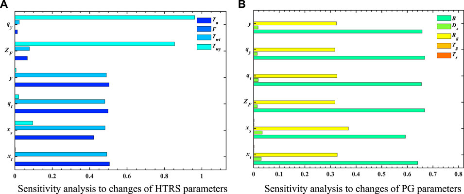
FIGURE 9. Sensitivity analysis to changes of HTRS and PG parameters. (A) Sensitivity analysis to changes of HTRS parameters. (B) Sensitivity analysis to changes of PG parameters.

FIGURE 10

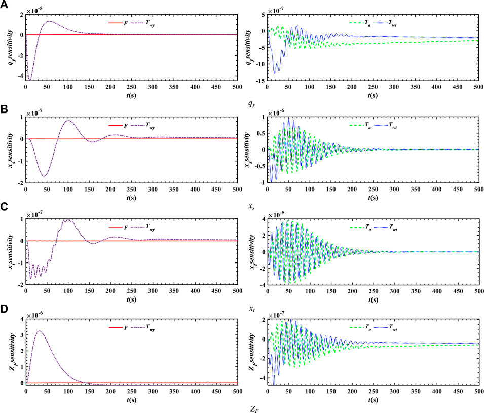
FIGURE 10. Sensitivity of HTRS parameters to state variables. (A) Sensitivity of HTRS parameters to state variable q_y. (B) Sensitivity of HTRS parameters to state variable x_s. (C) Sensitivity of HTRS parameters to state variable x_t. (D) Sensitivity of HTRS parameters to state variable Z_F.

Figure 9A describes the sensitivity analysis to changes of HTRS parameters at m_g = −0.1, K_p = 1, and K_i = 0.1. It can be seen from Figure 9A that the highest standard deviations of q_y and Z_F are correlated with T_wy while the highest standard deviations of y, q_t, x_s, and x_t are correlated with T_wt and T_a.

The sensitivity of HTRS parameters to state variables is shown in Figure 10. From Figure 10, it can be concluded that the state variables q_y and Z_F are more influenced by T_wy while effects of T_wt and T_a on the state variables x_s and x_t are more significant. Thus, q_y and Z_F are most sensitive to T_wy, but x_s and x_t are most sensitive to T_wt and T_a.

5.2 Sensitivity analysis of PG parameters

This section studies the sensitivity of PG parameters to state variables. The specific research method and normalization are the same as in the previous section, and the system operates under load condition, i.e., m_g = −0.1, K_p = 1, and K_i = 0.1. Sensitivity analysis to changes of PG parameters is shown in Figure 9B.

According to Figure 9B, state variables of the coupled system are most sensitive to parameters B and R_g, while the uncertainty sources of other parameters are less important. The results show that state variables are most sensitive to variability of B and R_g.

The sensitivity of PG parameters to state variables is shown in Figure 11. Since the sensitivity of PG parameters to state variables is not in the same order of magnitude, it is divided into two sub-graphs for better visualization. From Figure 11, it can be seen that q_y, x_s, x_t, and Z_F exhibited most sensitivity to the variation of B and R_g, while other parameters are less sensitive.

FIGURE 11

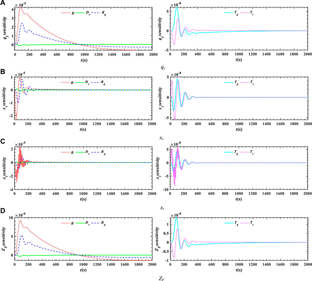
FIGURE 11. Sensitivity of PG parameters to state variables. (A) Sensitivity of PG parameters to state variable q_y. (B) Sensitivity of PG parameters to state variable x_s. (C) Sensitivity of PG parameters to state variable xt. (D) Sensitivity of PG parameters to state variable Z_F.

From Figures 10, 11, it can be concluded that the overall effect of the variation of HTRS parameters on x_t is greater than that of the variation of PG parameters. On the contrary, the overall effect of variable PG parameters on q_y, x_s, and Z_F is greater than that of variable HTRS parameters.

6 Conclusion

To reveal the impact mechanism of the hydropower station to the PG, the non-linear mathematical model considering a downstream surge chamber and sloping roof tailrace tunnel is established in this paper. Then, the Runge–Kutta method and Hopf bifurcation theory are applied to research the stability and dynamics characteristics of the coupled system, which are validated by numerical simulations. Furthermore, the coupling effects of different HTRS parameters and PG parameters on the coupled system are investigated and validated with phase space trajectory and dynamic response. Subsequently, the effect mechanism of governor parameters on the coupled system stability is revealed by eigenvalue analysis of the Jacobian matrix. Finally, the correlation between system state variables and parameters is verified through sensitivity analysis.

Based on the numerical analysis in this paper, conclusions can be drawn as follows:

(1) The non-linear mathematical model for the coupled system is an eighth-order non-linear state-space equation that considers the downstream surge chamber and the sloping roof tailrace tunnel. Afterward, by employing Hopf bifurcation theory, the stability and dynamics of the coupled system are analyzed effectively.

(2) With the coupled system under load perturbation, the whole K_p–K_i plane is divided into two parts by the bifurcation line consisting of bifurcation points. The stable domain is located at the lower end of the curve, while the unstable domain comprises the rest of the curve. Accordingly, the coupled system is stabilized at the equilibrium point when the state point lies in the stable domain.

(3) The stability of the coupled system can be enhanced by reducing the cross-sectional area of the downstream surge chamber, although the effect is limited. The unit inertia time constant and flow inertia time constant of the pressure pipeline can be employed as the main measures to optimize the dynamic performance of the coupled system.

(4) PG parameters can be reasonably regulated to optimize dynamic performance according to its impact on the coupled system. In addition, the influence mechanism of governor parameters on the stability of the coupled system is determined by analyzing eigenvalues of the Jacobian matrix.

(5) The sensitivity of the coupled system is greatly affected by the variation of HTRS and PG parameters. Furthermore, the overall effect of HTRS parameters on the sensitivity of the system state variables is greater than that of PG parameters. Based on sensitivity analysis, it can be concluded that the coupled system is most sensitive to T_a, T_wt, B, and R_g.

Data availability statement

The data analyzed in this study are subject to the following licenses/restrictions: The simulation data used to support the findings of this study are available from the corresponding author upon request. Requests to access these datasets should be directed to ZZ, dkyzhongziwei@163.com.

Author contributions

Conceptualization: ZZ and LZ; methodology: ZZ and MZ; software: JQ and SZ; validation: SZ and XC; resources: ZZ; writing—original draft preparation: SZ and XC; and writing—review and editing: XC. All authors contributed to the article and approved the submitted version.

Funding

This work is supported by the science and technology project of State Grid Shandong Eectric Power Research Institute (ZY-2023-08), which studies Research on online monitoring technology for safety warning of pumped storage power plants.

Conflict of interest

The authors declare that the research was conducted in the absence of any commercial or financial relationships that could be construed as a potential conflict of interest.

Publisher’s note

All claims expressed in this article are solely those of the authors and do not necessarily represent those of their affiliated organizations, or those of the publisher, the editors, and the reviewers. Any product that may be evaluated in this article, or claim that may be made by its manufacturer, is not guaranteed or endorsed by the publisher.

References

Chaudhry, M. H. (2014). Applied hydraulic transients. 3rd ed. New York: Springer-Verlag.

Google Scholar

Feng, C., and Chang, L. (2018). Robust takagi-sugeno fuzzy control for nonlinear singular time-delay hydraulic turbine governing system. Proc. - 2018 11thInt Symp. Comput. Intell. Des. Isc 2, 249–253.

CrossRef Full Text | Google Scholar

Fu, W., Zhang, S., Zheng, Y., et al. (2023). Dynamic sliding mode control of hydraulic turbine governing system. China Rural Water Hydropower 2023 (02), 211–217.

Google Scholar

Guo, P., Zhang, Y., and Chen, W. (2023). Numerical analysis on a self-rectifying impulse turbine with U-shaped duct for oscillating water column wave energy conversion. Energy 274, 127359. doi:10.1016/j.energy.2023.127359

CrossRef Full Text | Google Scholar

Guo, W., and Peng, Z. (2020). Order reduction and dynamic performance of hydropower system with surge tank for grid-connected operation. Sustain Energy Technol. Assessments 40, 100777. doi:10.1016/j.seta.2020.100777

CrossRef Full Text | Google Scholar

Guo, W., and Yang, J. (2018). Dynamic performance analysis of hydro-turbine governing system considering combined effect of downstream surge tank and sloping ceiling tailrace tunnel. Renew. Energy 129, 638–651. doi:10.1016/j.renene.2018.06.040

CrossRef Full Text | Google Scholar

Guo, W., Yang, J., Wang, M., and Lai, X. (2015). Nonlinear modeling and stability analysis of hydro-turbine governing system with sloping ceiling tailrace tunnel under load disturbance. Energy Convers. Manag. 106, 127–138. doi:10.1016/j.enconman.2015.09.026

CrossRef Full Text | Google Scholar

Hassard, B. D., Kazarinoff, N. D., and Wan, Y. W. (1981). Theory and applications of Hopf bifurcation. London: Cambridge University Press.

Google Scholar

Lai, X., Li, C., Guo, W., Xu, Y., and Li, Y. (2019). Stability and dynamic characteristics of the nonlinear coupling system of hydropower station and power grid. Commun. Nonlinear Sci. Numer. Simul. 79, 104919. doi:10.1016/j.cnsns.2019.104919

CrossRef Full Text | Google Scholar

Liu, D., Li, C., and Malik, O. P. (2021). Nonlinear modeling and multi-scale damping characteristics of hydro-turbine regulation systems under complex variable hydraulic and electrical network structures. Appl. Energy 293, 116949. doi:10.1016/j.apenergy.2021.116949

CrossRef Full Text | Google Scholar

Liu, L., Wang, B., Wang, S., Chen, Y., Hayat, T., and Alsaadi, F. E. (2018). Finite-Time H-Infinity control of a fractional-order hydraulic turbine governing system. IEEE Access 6, 57507–57517. doi:10.1109/access.2018.2873769

CrossRef Full Text | Google Scholar

Liu, Y., and Guo, W. (2021). Multi-frequency dynamic performance of hydropower plant under coupling effect of power grid and turbine regulating system with surge tank. Renew. Energy 171, 557–581. doi:10.1016/j.renene.2021.02.124

CrossRef Full Text | Google Scholar

Lu, X., Li, C., Liu, D., Zhu, Z., Tan, X., and Xu, R. (2022). Comprehensive stability analysis of complex hydropower system under flexible operating conditions based on a fast stability domain solving method. SSRN Electron J. 274, 127368. doi:10.1016/j.energy.2023.127368

CrossRef Full Text | Google Scholar

Ma, T., and Wang, B. (2021). Disturbance observer-based Takagi-Sugeno fuzzy control of a delay fractional-order hydraulic turbine governing system with elastic water hammer via frequency distributed model. Inf. Sci. (Ny) 569, 766–785. doi:10.1016/j.ins.2021.05.013

CrossRef Full Text | Google Scholar

Ma, T., Wang, B., Zhang, Z., and Ai, B. (2021). A Takagi-Sugeno fuzzy-model-based finite-time H-infinity control for a hydraulic turbine governing system with time delay. Int. J. Electr. Power Energy Syst. 132, 107152. doi:10.1016/j.ijepes.2021.107152

CrossRef Full Text | Google Scholar

Piraisoodi, T., Maria Siluvairaj, W. I., and Kappuva, M. A. K. (2019). Multi-objective robust fuzzy fractional order proportional–integral–derivative controller design for nonlinear hydraulic turbine governing system using evolutionary computation techniques. Expert Syst. 36, 123666–e12415. doi:10.1111/exsy.12366

CrossRef Full Text | Google Scholar

Shi, K., Wang, B., and Chen, H. (2018). Fuzzy generalised predictive control for a fractional-order nonlinear hydro-turbine regulating system. IET Renew. Power Gener. 12, 1708–1713. doi:10.1049/iet-rpg.2018.5270

CrossRef Full Text | Google Scholar

Strogatz, S. H. (2014). Nonlinear dynamics and chaos: With applications to physics, biology, chemistry, and engineering. Second Edi. Boulder: Westview Press.

Google Scholar

Tian, Y., Wang, B., Chen, P., and Yang, Y. (2020). A state estimator–based nonlinear predictive control for a fractional-order Francis hydraulic turbine governing system. JVC/Journal Vib. Control 26, 1068–1080. doi:10.1177/1077546319891633

CrossRef Full Text | Google Scholar

Tian, Y., Wang, B., Chen, P., and Yang, Y. (2021). Finite-time Takagi–Sugeno fuzzy controller design for hydraulic turbine governing systems with mechanical time delays. Renew. Energy 173, 614–624. doi:10.1016/j.renene.2021.04.011

CrossRef Full Text | Google Scholar

Tian, Y., Wang, B., Zhu, D., and Wu, F. (2019). Takagi-Sugeno fuzzy generalised predictive control of a time-delay non-linear hydroturbine governing system. IET Renew. Power Gener. 13, 2338–2345. doi:10.1049/iet-rpg.2019.0329

CrossRef Full Text | Google Scholar

Wang, B., Xue, J., Wu, F., and Zhu, D. (2018). Finite time takagi-sugeno fuzzy control for hydro-turbine governing system. JVC/Journal Vib. Control 24, 1001–1010. doi:10.1177/1077546316655912

CrossRef Full Text | Google Scholar

Wiggins, S. (2013). Global bifurcations and chaos: Analytical methods. Vol. 73. Berlin: Springer Science & Business Media.

Google Scholar

Wu, F., Li, F., Chen, P., and Wang, B. (2019). Finite-time control for a fractional-order non-linear HTGS. IET Renew. Power Gener. 13, 633–639. doi:10.1049/iet-rpg.2018.5734

CrossRef Full Text | Google Scholar

Xu, P., Fu, W., Lu, Q., Zhang, S., Wang, R., and Meng, J. (2023). Stability analysis of hydro-turbine governing system with sloping ceiling tailrace tunnel and upstream surge tank considering nonlinear hydro-turbine characteristics. Renew. Energy 210, 556–574. doi:10.1016/j.renene.2023.04.028

CrossRef Full Text | Google Scholar

Xu, X., and Guo, W. (2020). Stability of speed regulating system of hydropower station with surge tank considering nonlinear turbine characteristics. Renew. Energy 162, 960–972. doi:10.1016/j.renene.2020.08.098

CrossRef Full Text | Google Scholar

Xu, Y., Zheng, Y., Du, Y., Yang, W., Peng, X., and Li, C. (2018). Adaptive condition predictive-fuzzy PID optimal control of start-up process for pumped storage unit at low head area. Energy Convers. Manag. 177, 592–604. doi:10.1016/j.enconman.2018.10.004

CrossRef Full Text | Google Scholar

Yang, J., Mu, A., and Li, N. (2019a). Dynamical analysis and stabilization of wind turbine drivetrain via adaptive fixed-time terminal sliding mode controller. Math. Problems Eng. 2019, 1–14. doi:10.1155/2019/8982028

CrossRef Full Text | Google Scholar

Yang, W., Yang, J., Zeng, W., Tang, R., Hou, L., Ma, A., et al. (2019b). Experimental investigation of theoretical stability regions for ultra-low frequency oscillations of hydropower generating systems. Energy 186, 115816. doi:10.1016/j.energy.2019.07.146

CrossRef Full Text | Google Scholar

Yi, Y., and Chen, D. (2019). Disturbance observer-based backstepping sliding mode fault-tolerant control for the hydro-turbine governing system with dead-zone input. ISA Trans. 88, 127–141. doi:10.1016/j.isatra.2018.11.032

PubMed Abstract | CrossRef Full Text | Google Scholar

Yi, Y., Chen, D., Li, H., Li, C., and Zhou, J. (2020). Observer-based adaptive output feedback fault tolerant control for nonlinear hydro-turbine governing system with state delay. Asian J. Control 22, 192–203. doi:10.1002/asjc.1859

CrossRef Full Text | Google Scholar

Zhang, F., Fang, M., Pan, J., Tao, R., Zhu, D., Liu, W., et al. (2023b). Guide vane profile optimization of pump-turbine for grid connection performance improvement. Energy 274, 127369. doi:10.1016/j.energy.2023.127369

CrossRef Full Text | Google Scholar

Zhang, H., Chen, D., Wu, C., Wang, X., Lee, J. M., and Jung, K. H. (2017). Dynamic modeling and dynamical analysis of pump-turbines in S-shaped regions during runaway operation. Energy Convers. Manag. 138, 375–382. doi:10.1016/j.enconman.2017.01.053

CrossRef Full Text | Google Scholar

Zhang, W., Chen, Y., Wang, Y., and Xu, Y. (2023d). Equilibrium analysis of a peer-to-peer energy trading market with shared energy storage in a power transmission grid. Energy 274, 127362. doi:10.1016/j.energy.2023.127362

CrossRef Full Text | Google Scholar

Zhang, Y., Le, W., Fu, W., Chen, X., and Hu, S. (2023c). Secondary frequency control strategy considering DoS attacks for MTDC system. Electr. Power Syst. Res. 214, 108888. doi:10.1016/j.epsr.2022.108888

CrossRef Full Text | Google Scholar

Zhang, Y., Xie, X., Fu, W., Chen, X., Hu, S., Zhang, L., et al. (2023a). An optimal combining attack strategy against economic dispatch of integrated energy system. IEEE Trans. Circuits Syst. II Express Briefs 70 (1), 246–250. doi:10.1109/tcsii.2022.3196931

CrossRef Full Text | Google Scholar

Zhao, Z., Yang, J., Chung, C. Y., Yang, W., He, X., and Chen, M. (2021b). Performance enhancement of pumped storage units for system frequency support based on a novel small signal model. Energy 234, 121207. doi:10.1016/j.energy.2021.121207

CrossRef Full Text | Google Scholar

Zhao, Z., Yang, J., Huang, Y., Yang, W., Ma, W., Hou, L., et al. (2021a). Improvement of regulation quality for hydro-dominated power system: quantifying oscillation characteristic and multi-objective optimization. Renew. Energy 168, 606–631. doi:10.1016/j.renene.2020.12.084

CrossRef Full Text | Google Scholar

Zheng, Y., Chen, Q., Yan, D., and Zhang, H. (2022). Equivalent circuit modelling of large hydropower plants with complex tailrace system for ultra-low frequency oscillation analysis. Appl. Math. Model 103, 176–194. doi:10.1016/j.apm.2021.10.017

CrossRef Full Text | Google Scholar

Zhu, D., and Guo, W. (2019). Setting condition of surge tank based on stability of hydro-turbine governing system considering nonlinear penstock head loss. Int. J. Electr. Power Energy Syst. 113, 372–382. doi:10.1016/j.ijepes.2019.05.061

CrossRef Full Text | Google Scholar

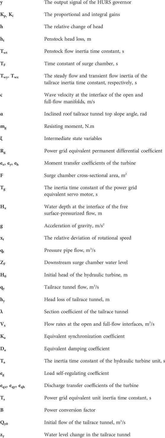
Nomenclature