A game strategy for demand response based on load monitoring in smart grid

Demand response technologies can achieve the objective of optimizing resource allocation and ensuring efficient operation of the smart grid by motivating the energy users to change their power usage behavior. However, the increasing uncertainty of smart grid environment brings great challenges to the development of demand response technique. In this study, we build a long short-term memory (LSTM) network as a load forecasting model to predict user load data in order to obtain accurate consumption behavior of energy users. Then, we utilize a Stackelberg game model based on the load forecasting model to dynamically optimize the electricity prices set by power suppliers at different times, enhancing the efficiency of demand response between users and suppliers. Extensive simulation experiments demonstrate that the LSTM-based load forecasting model achieves an accuracy of up to 96.37% in predicting user load demand. And the game model reduces the overall expenditure of users by 30% compared with the general pricing model.

1 Introduction

The concept of the smart grid stems from the idea of Advanced Metering Infrastructure (AMI). Its goal is to enhance demand-side management and energy efficiency and to construct a self-healing, reliable grid protection system capable of withstanding severe human-induced disruptions and potential natural disasters (Mahela et al., 2022). However, the rapid advancement of information technology has led the power industry and research institutions to reconsider and expand the initial vision of the smart grid, enabling the full utilization of information technology within smart grids (Orlando et al., 2022). Recently, the smart grid has evolved into a typical cyber-physical system (CPS), integrating electric power, information transmission, network security communication, and intelligent computing. It has established a clean, secure, efficient, and sustainable advanced energy delivery network (Gao et al., 2023). For instance, to reduce peak demand and smooth load curves, power suppliers can use the high-speed communication network of a smart grid to encourage specific users to reduce their load during peak periods using real-time pricing signals. This not only incentivizes users to participate in the grid regulation but also smooths the load curve, thereby improving the overall energy utilization rate (Trujillo and García Torres, 2022).

The smart grid with distributed power supply model greatly enhances the reliability and self-healing capabilities of power system, reducing the scope of power outages through self-healing responses (Jasim et al., 2023). In terms of economic benefits, the cost-to-benefit ratio of a smart grid is approximately 4:1–5:1 (Gellings et al., 2004). In addition to bringing substantial direct economic benefits to power companies, this saves a significant amount of energy, contributing to environmental protection and sustainable development in society. To achieve the aforementioned benefits and generate greater economic gains, it is necessary to invest more research effort in areas such as demand response and load supervision (Khan et al., 2023).

Load monitoring (LM) technology allows power suppliers to make predictions about user’s load usage and to learn about load usage patterns, which can be divided into intrusive and non-intrusive types based on the monitoring approach. Intrusive load monitoring requires the installation of measuring devices on each load, which leads to higher overall costs and lower usage frequency (Wang et al., 2020). Non-intrusive load monitoring, on the other hand, does not require installing measuring devices in each user’s home. Instead, the devices are installed at the power entry points of various centralized units to collect aggregated data. Subsequently, the aggregated energy loads are decomposed into individual energy loads, enabling a simple and effective way to forecast load operations and energy consumption (Abubakar et al., 2017).

In order to effectively encourage the participation of users in the electricity trading process, power suppliers often utilize demand response techniques to motivate the power users changing their inherent power consumption behavior by adopting certain incentives. The research efforts of demand response techniques can be divided into price-based and incentive-based. Price-based demand response techniques help power suppliers to learn autonomous pricing strategies to arrange loads of energy users (Liu et al., 2017). Tang et al. (2019) and Cheng et al. (2022) modelled the interaction strategies between power grid and energy users as a Stackelberg game model, in which the grid optimizes the price to maximize its net profit and reduce demand fluctuation, and individual energy user optimizes the hourly power demand to minimize electricity bill and effects of demand alternation from the baseline. Sofana Reka and Ramesh (2016) utilized a generalized tit for tat dominant game-based energy scheduler to shift the peak average ratio of the smart grid. While, incentive-based demand response techniques enable power suppliers to learn an economic compensation mechanism to encourage energy users reducing their peak-periods loads (Zheng et al., 2022). For instance, Mansouri et al. (2023) proposes a three-layer risk-averse game theoretic-based strategy to coordinate smart buildings and EV fleets with microgrids scheduling. In the first layer of above strategy, a demand response program is designed for smart buildings where dynamic incentive tariffs are calculated based on the consumption pattern of subscribers.

Although demand response techniques have been widely deployed in addressing the resource allocation problem of smart grid (Sivasankarareddy et al., 2021; Panda et al., 2022). However, there remaining some obstacles that prevent above methods from implementing in realistic scenarios. 1) The increasing uncertainty of users loads brings great challenges to the establishment of accurate optimization model, resulting in the inefficiency of demand response strategies. 2) Existing game model-based demand response strategies lack the theoretical analysis of Nash equilibrium. Differently, this paper investigates a demand response model integrates load monitoring technology. In this demand response model, the interaction between power suppliers and users is modeled using game theory. Each power supplier dynamically adjusts its price signal based on the user’s demand, while users passively respond to the price signal by submitting their demand signals, ultimately maximizing the utility of user and profit of power supplier. The main contributions are as follows:

• This paper employs LSTM networks as the load forecasting model to predict user load data based on the load forecasting model and demand response theory. The LSTM network, with its memory units, can effectively capture historical load data and learn the periodic patterns in user load data.

• This paper designs a demand response model based on Stackelberg game theory, utilizing the load prediction results from the load forecasting model. This model accurately represents the complex demand response interaction between users and power suppliers in the smart grid. Mathematical derivations demonstrate that the entire interaction process can reach a Nash equilibrium, which can maximize the utility of both parties.

• This paper presents extensive simulation experiments to demonstrate the effectiveness of both the load forecasting model and demand response model. Simulation results prove that the LSTM-based load forecasting model can achieve up to 96.37% accuracy in load demand prediction for users. And the proposed game model can significantly reduce users’ electricity expenses.

The main notations utilized in this paper are summarized in Table 1.

TABLE 1

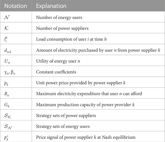
TABLE 1. Main notations.

2 Related work

2.1 Research status of load monitoring models in smart grids

Load supervision is a key technology that predicts future energy demand based on historical load data, temperature data, and weather data. The prediction of future demand from load supervision is a critical parameter for the operation and planning of a power system. Errors between the predictive model and the actual parameters can lead to increased operational costs and later increased costs for power suppliers. Hence, many load supervision models have been proposed to achieve more precise load demand prediction. Current research on load supervision models by scholars worldwide can be classified into two categories: models based on probability and statistics and models based on artificial intelligence.

Regarding probabilistic-statistical models (Huang and Shih, 2003), presents a variety of statistical models. These include the autoregressive model (AR), moving average model (MA), autoregressive moving average model (ARMA), and autoregressive integrated moving average model (ARIMA), with detailed explanations of each model’s mathematical expression and prediction methods. Hermias et al. (2017) uses an ARIMA model to predict future air-conditioning load based on seasonal component compensation. Alhmoud and Nawafleh (2021) used ARMA method and two neural network-based methods to predict the load data. Through simulation, it was demonstrated that the neural network approach could effectively improve the prediction accuracy. Among artificial intelligence-based load supervision models, Walther et al. (2019) proposed a very short-term load data predictor based on machine learning. It simply used a single-step delay, taking only the current value and time load data of the single-step delay as input to predict future load data. Mocanu et al. (2016) aimed to improve the design of power infrastructure and the effective deployment of distributed and renewable energy sources by predicting the electricity consumption patterns in power systems through a deep learning network, thereby enhancing the electricity efficiency of the entire power system. The authors creatively proposed the conditional restricted Boltzmann machine (CRBM) and factor conditional restricted Boltzmann machine (FCRBM) models to predict data and validated their accuracy through simulation experiments. Afrasiabi et al. (2020) mainly proposed a hybrid predictive model based on convolution neural networks to predict residential power load curves. By predicting the loads of individual users, the power supply system can better monitor electricity usage habits, thus achieving better load scheduling.

2.2 Research status of demand response technology in smart grids

Compared with traditional power grids, the advantage of smart grids is that they can significantly improve the reliability of the entire power system and the responsiveness of users and can encourage users to participate more actively in energy trading decisions. Therefore, all scheduling and incentives on the demand side, including overall demand response management, are integral parts of the smart grid. Current demand response mechanisms can be divided into two categories: one is based on user incentive mechanisms, and the other is based on power pricing mechanisms.

Gyamfi et al. (2013) studied different demand response mechanisms, such as time-of-use (TOU) pricing, peak pricing, and real-time pricing, and applied them to users in different countries and regions to measure their response rates to these mechanisms. This laid a solid foundation for later research on demand response theories. The results showed that a large portion of households did not respond to price changes, possibly because they did not understand the pricing system and therefore did not react immediately to price changes. Zhang et al. (2023) proposed a demand response algorithm based on bidding incentives. This algorithm used Vickrey-Clarke-Groves mechanism to optimize the choice of energy policies to find the strategy that maximizes the total profit of the energy service provider while satisfying the user’s minimum load power requirements. Trujillo and García Torres (2022) proposed a multi-stage control system to manage the electric vehicle users’ demand, automatically adjust the load, and optimize the entire system using a stochastic optimization algorithm. This study provided the best demand response solutions for users by comparing various strategies based on pricing mechanism and incentive mechanism. Bokkisam et al. (2022) proposed a peer-to-peer demand transactive system. In this algorithm, the smart grid was divided into three agents: users, auctioneer, and utility. To consider the balance of user benefits, load demand, and energy supply, the third-party agent demonstrated method and blockchain-based method were tested. The optimal real-time demand allocation results was obtained through simulation experiments.

In summary, based on the current research status worldwide, the problem of demand response models based on load supervision in smart grids is a frontier issue that crosses multiple fields. Although many theories and results have been obtained in various fields, better integrating load supervision methods with demand response models to ensure the stability of overall system operation while achieving satisfactory returns between users and power suppliers is a subject that urgently needs to be studied.

3 Preliminaries

3.1 System model

The model of the game demand response strategy based on load demand forecasting studied in this paper includes two main entities: the power supplier and the users. Within the energy management unit, there are multiple power suppliers, each with varying capacities due to their different scales. However, each power supplier can independently supply electric power to users. Compared to the centralized power supply of traditional grids, this distributed power supply from multiple suppliers greatly enhances the stability and robustness of the entire power system. Each power supplier, constrained by its capacity and costs, sets real-time prices at each moment, resulting in different prices among suppliers. Users can choose to purchase electric power from the supplier that maximizes their own utility based on their load usage habits.

In the demand response strategy, the power suppliers first use the trained load demand prediction model to forecast the future load demand of each user. They then issue an initial electricity price signal to the users based on the predicted load demand. During this process, the prices set by each supplier differ based on the users’ load demand and the suppliers’ capacities and costs. Upon receiving the price signal, users calculate the optimal energy demand from different suppliers based on their maximum energy cost expenditure and a utility optimization function. They then send the demand signals to the respective suppliers. Each supplier receives the energy demand purchased by users, and being rational and self-interested, adjusts its electricity price information to maximize its own revenue. This forms a non-cooperative game model among the power suppliers. This entire demand response process continues until the system reaches a Nash equilibrium. At equilibrium, no power supplier can increase its revenue by unilaterally changing its price information.

3.2 Game theory approach

Game theory is a formal analytical framework that studies complex interactions among independent rational players using specific mathematical representations and derives the optimal strategies of the players based on individual rational behavior. Over the decades, game theory has been widely applied in various disciplines, ranging from economics and political science to psychology, achieving significant progress across different fields. In today’s large-scale smart grid systems and various cyber-physical systems (CPSs), complex interactions often exist among multiple intelligent nodes. To achieve better interactions between power suppliers and users, the framework of game theory has become an important theoretical analysis tool and has been widely applied in practical optimization scenarios (Cheng and Yu, 2019). Game models typically consist of three elements: players $\mathcal{N}$, decision sets ${({\mathcal{A}}_i)}_{i\in \mathcal{N}}$, and utility functions ${(U_i)}_{i\in \mathcal{N}}$. In the entire non-cooperative static game process, each decision maker i aims to select a decision process $a_i\in {\mathcal{A}}_i$ from their decision set ${\mathcal{A}}_i$ to maximize their own utility function U_i(a_i, a − i). However, the utility function of a user depends not only on their own decision a_i but also on the decisions a_−i of participants other than user i. As each user seeks to maximize their own utility, a game model is formed accordingly.

The aforementioned game model can be applied to demand response management in smart grids. A smart grid system has $\mathcal{N}$ users and multiple power suppliers. In a given period h, the total load consumption of all users in the system can be represented as $L_h={\sum }_{i\in N}{l}_i^h$, where $l_i^h$ represents the load consumption of user i at time h. When users consume electricity, power suppliers bear costs associated with electricity production and transmission. The overall costs can be represented by a cost function C_h = ∑_i∈NC_h(L_h), where the cost function is a strictly increasing convex function with the user’s load consumption as the independent variable. When the load consumption of users at a certain time is higher, the value of the cost function also increases. Therefore, power suppliers determine the electricity price at time h based on the magnitude of the cost function. A larger cost function indicates higher costs, resulting in a higher electricity price being set, and vice versa. The size of the cost function mainly depends on the consumption L_h at that time. When a user participating in scheduling changes their load consumption, it affects the current consumption L_h, which in turn influences the power supplier’s setting of the electricity price through C_h. In other words, in each period, users can influence the electricity price of the entire system by scheduling their own loads. The less load consumption in the system, the lower the power supplier will set the electricity price, and the more load consumption in the system, the higher the power supplier will set the electricity price. If each user wants a lower electricity price when using their load, a game model arises. The participants are all the users N involved in scheduling, the decision set is the load consumption l_h of each user at a certain time, and the utility function represents each user’s desire to maximize their own utility through the scheduling of their load. When the entire game model reaches a Nash equilibrium, no user in the system can improve their own utility simply by changing their load consumption decision, resulting in an equilibrium state for the entire system.

4 Load supervision method based on an LSTM network

In recent years, the rapid development of information technology has led to the widespread application of smart grids. In a smart grid, the integration of various renewable energy supply nodes, electric vehicle nodes, and user access nodes significantly increases the complexity and instability of the entire system. Undoubtedly, compared to the centralized energy supply in traditional grids, the access of various distributed nodes in smart grids poses unprecedented challenges to system stability. To address this issue, load supervision technology has been widely applied in practical projects. Through load supervision technology, it is possible to assist in demand response and achieve the transfer of peak demand, thereby improving the overall stability of the system. In the field of load supervision, deep learning techniques have begun to be widely used. Deep learning utilizes multilayer neural connections to extract features from input data. Compared to traditional machine learning algorithms, deep learning greatly improves the accuracy of models and enhances prediction accuracy through stacking layers and increasing the number of neurons.

4.1 LSTM network

Although classical feedforward fully connected neural networks work well for traditional data classification and regression problems, they face challenges when dealing with continuous sequential data such as time series load data and speech data. This is because sequential data have inherent order dependencies, and it is not straightforward to split these time series data into independent training samples to train a traditional feedforward neural network. Therefore, to consider the sequential nature of the data during training, adjustments need to be made to the structure of the traditional feedforward neural network by introducing memory units, giving rise to RNNs. Long short-term memory (LSTM) networks are a type of neural network architecture proposed to address the issue of vanishing gradients in RNNs (Cai et al., 2022). Compared to traditional RNN architectures, LSTM incorporates dedicated memory modules to retain previous information. In terms of the update mechanism, LSTM does not directly overwrite the information in the memory unit with the sequence information obtained at the previous time step. Instead, it accumulates information over time, ensuring the retention of information from much earlier sequences. Figure 1 represents a basic LSTM unit, which includes three crucial gate structures: the input gate, the output gate, and the forget gate. The input gate determines whether the current information x_t should be stored in memory cell s_t. The output gate determines whether the current information in memory cell s_t should be output as the current output h_t. The forget gate controls how much information from the previous memory cell s_t−1 should be stored in the current memory cell s_t.

FIGURE 1

FIGURE 1. LSTM network unit structure.

4.2 Construction of a load monitoring model based on an LSTM network

4.2.1 Load data analysis

After obtaining the load consumption data, the first step is to perform data cleaning, which includes handling outliers and missing values in the data. Then, the correlation between different features needs to be examined. Since the dataset in this study has many features, using all of them as training data would result in an excessively high dimensionality of the training dataset. Moreover, for time series data, when constructing the supervised model data, a certain time step delay is applied, which further increases the number of features, leading to a significant computational burden and prolonged training time. Therefore, to address this issue, it is necessary to eliminate some highly correlated feature attributes through correlation analysis, aiming to improve training speed without compromising model accuracy.

Through correlation analysis, it is found that there is a strong correlation between various features. In this study, temperature and humidity are selected as the training data features (Chen et al., 2021). Additionally, since user load consumption is often related to user behavior patterns, with lower consumption during weekdays and higher consumption during weekends, this study uses an additional feature to represent whether the current date is a weekend in training the model.

4.2.2 Load supervision model framework

The load supervision model is primarily built using LSTM networks and trained with the historical load data obtained in the previous section.

The construction steps of the entire model are as follows:

1) Encode the vector data W indicating whether it is a working day, where 1 represents a working day and 0 represents a weekend.

2) Normalize the load data L, temperature data T, and humidity data H, and then concatenate these vectors to form the input matrix X = {T, H, W, L}.

3) Transform the preprocessed time series data X into data suitable for supervised learning based on the designated time step K. By using a sliding window approach, the input matrix X is shifted with a step size.

4) Input the matrix X into the LSTM network for model training.

The framework of the entire model is shown in Figure 2.

FIGURE 2

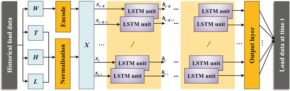
FIGURE 2. Load supervision model framework.

5 Demand response methods based on game theory

In traditional demand response models, due to the complex interaction between users and the power supply side, the optimization process often only considers one side of the demand response. For instance, when considering the maximization of user welfare, the maximization of the power supply side’s benefits is not included. To model the complex interaction process between multiple users and multiple power suppliers in the demand response, this section studies a model based on a Stackelberg game as shown in Figure 3. First, each power supplier predicts the future load demand of users using the load demand prediction model proposed in the previous section and determines the initial electricity price based on the current load demand and its own power supply. Then, each user compares the price signals provided by all power suppliers to maximize their own benefits, purchases electricity from different power suppliers according to their own electricity usage habits, and synchronizes the demand information in real time to the designated power supplier. Finally, the power supplier updates its price signal based on the user’s purchased demand and the price signals of the other power suppliers.

FIGURE 3

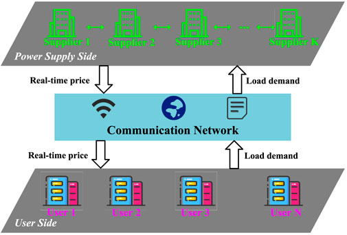
FIGURE 3. Demand response system model.

In the entire demand response model, $\mathcal{N}=\{\mathrm{1,2},\dots ,N\}$ represents the number of users, and $\mathcal{K}=\{\mathrm{1,2},\dots ,K\}$ represents the number of power suppliers. The entire system model is shown in Figure 3. The power supply side of this model includes the connection of various renewable and non-renewable energy suppliers. Non-renewable energy includes various fossil fuels, which produce relatively stable electricity and can continuously output electricity. However, due to the pollution caused by the combustion of such fuels and their non-renewable nature, an increasing amount of renewable clean energy is connected to the grid. On the user side, various types of users, such as residential users, industrial users, and commercial users, are distinguished by their set load demand limits. When modeling power suppliers and users, users express the utility value obtained after consuming electricity through a utility function, and power suppliers express the profit obtained after selling electricity through a profit function. The communication between the two parties is carried out through the two-way communication network, where each power supplier sends its price signal to the users in real time, and the users respond to the demand signal of the power supplier considering the maximization of their own utility after receiving different price signals.

The entire interaction process of the demand response model constitutes a Stackelberg game. In this game process, the power supplier, as a leader, sends the real-time price signal to the followers first, while the user, as a follower, optimizes their load demand allocation according to the price signal issued by the leader. Therefore, the entire game process can be seen as a game of electricity prices among various power suppliers. The power suppliers set their own electricity prices according to the amount of user loads and the price levels of other power suppliers, while the users passively respond, maximizing their own utility functions through the real-time price signals issued by the power suppliers.

5.1 User-side mathematical model

The entire system architecture involves multiple users and multiple power suppliers, where each user $n\in \mathcal{N}$ selects the amount of electricity purchased d_n,k ≥ 0 according to the price signal released by each power supplier $k\in \mathcal{K}$ at each unit time. The unit time is set to 30 min, and the user’s energy demand purchase volume maximizes the utility function under the premise of satisfying its own cost budget. In this article, the utility functions of users at the unit time can be represented as:

$U_n\left({\mathit{d}}_{\mathit{n}}\right)={\gamma }_n\sum _{k\in \mathcal{K}}\ln \left({\beta }_n+d_{n,k}\right)(1)$

where γ_n > 0 and β_n ≥ 1 are both constant coefficients. These coefficients ensure that when the user does not purchase electricity from any power supplier, that is, when d_n = 0, the value of the formula ${\sum }_{k\in \mathcal{K}}\ln (d_{n,k})$ will not reach −∞. In Eq. 1, the user’s utility is modeled through a logarithmic function (Wang et al., 2021).

The user’s goal is to maximize their utility function while first satisfying their own budget by determining their electricity demand purchases based on their own electricity consumption habits and the prices of different power suppliers. The optimization function can be expressed as:

$\begin{array}{cc}\hfill & {\max }_{{\mathit{d}}_n}{U}_n\left({\mathit{d}}_n\right)\hfill \\ \hfill & s.t.\left\{\begin{array}{c}\sum _{k\in \mathcal{K}}{p}_k{d}_{n,k}\le B_n\hfill \\ d_{n,k}\ge 0,\forall k\in \mathcal{K}\hfill \end{array}\right.\hfill \end{array}(2)$

where p_k represents the real-time unit power price provided by power supplier k and B_n represents the maximum electricity expenditure that user n can afford. The optimization process on the user side does not involve a game between users; they only passively accept the price signals provided by the power supplier to maximize their utility functions. Each user’s decision can be considered as being made independently.

To understand the energy demand optimization process on the user side more clearly, this article first assumes a general situation: there are only N users and three power suppliers in the demand response management system. After careful analysis of the general situation, the conclusion is extended to $\mathcal{K}$ power suppliers. When there are only three power suppliers in the system, the optimization problem can be expressed as:

$\begin{array}{cc}\hfill & \underset{d_{n,1},d_{n,2},dn,3}{\max }{\gamma }_n\sum _{k=1}^3\ln \left({\beta }_n+d_{n,k}\right)\hfill \\ \hfill & s.t.\left\{\begin{array}{c}{p}_1{d}_{n,1}+p_2{d}_{n,2}+p_3{d}_{n,3}\le B_n\hfill \\ d_{n,1},d_{n,2},d_{n,3}\ge 0\hfill \end{array}\right.\hfill \end{array}(3)$

Introducing the Lagrange multipliers λ_n,1, λ_n,2, λ_n,3, λ_n,4, the optimization problem with inequality constraints is represented by a Lagrange function as follows:

$\begin{array}{cc}\hfill {\mathcal{L}}_n=& {\gamma }_n\sum _{k=1}^3\ln \left({\beta }_n+d_{n,k}\right)-{\lambda }_{n,1}\left(\sum _{k=1}^3{p}_k{d}_{n,k}-B_n\right)\hfill \\ \hfill & +{\lambda }_{n,2}{d}_{n,1}+{\lambda }_{n,3}{d}_{n,2}+{\lambda }_{n,4}{d}_{n,3}\hfill \end{array}(4)$

The KKT conditions are:

${\lambda }_{n,1}\left(\sum _{k=1}^3{p}_k{d}_{n,k}-B_n\right)=0(5)$

${\lambda }_{n,2}{d}_{n,1}=0(6)$

${\lambda }_{n,3}{d}_{n,2}=0(7)$

${\lambda }_{n,4}{d}_{n,3}=0(8)$

${\lambda }_{n,1}>0(9)$

${\lambda }_{n,2},{\lambda }_{n,3},{\lambda }_{n,4}\ge 0(10)$

$x_{n,1},x_{n,2}\ge 0(11)$

When the utility function is maximized, the first derivative of Eq. 4 needs to be zero; that is, $\nabla {\mathcal{L}}_n({\mathit{d}}_n^{*})=0$. The partial derivative of Eq. 4 can be obtained as:

$\left\{\begin{array}{cc}\frac{{\gamma }_n}{{\beta }_n+d_{n,1}}-{\lambda }_{n,1}{p}_1+{\lambda }_{n,2}\hfill & \hfill =0\hfill \\ \frac{{\gamma }_n}{{\beta }_n+d_{n,2}}-{\lambda }_{n,1}{p}_2+{\lambda }_{n,3}\hfill & \hfill =0\hfill \\ \frac{{\gamma }_n}{{\beta }_n+d_{n,3}}-{\lambda }_{n,1}{p}_3+{\lambda }_{n,4}\hfill & \hfill =0\hfill \end{array}\right.(12)$

To determine the optimal amount of energy for each user to purchase from each power supplier at this time, the amount of electrical energy purchased by users from each power supplier needs to be considered in categories:

1) When d_n,1 > 0, d_n,2 > 0, d_n,3 > 0:

Through Eqs 6–8, we can derive λ_n,2 = λ_n,3 = λ_n,4 = 0. Substituting λ_n,2, λ_n,3, and λ_n,4 into Eq. 12, we obtain:

$d_{n,k}=\frac{{\gamma }_n}{{\lambda }_{n,1}{p}_k}-{\beta }_n\forall n\in \mathcal{N},k=\mathrm{1,2,3}.(13)$

Substituting Eq. 13 into Eq. 5, we can solve for:

${\lambda }_{n,1}=\frac{3{\gamma }_n}{B_n+{\sum }_{k=1}^3{p}_k{\beta }_n}(14)$

Finally, by substituting Eq. 14 into Eq. 13, we can solve for the amount of electricity each user purchases from each power supplier:

$d_{n,k}=\frac{B_n+{\sum }_{k=1}^3{p}_k{\beta }_n}{3p_k}-{\beta }_{n}k=\mathrm{1,2,3}.(15)$

2) When d_n,1 > 0, d_n,2 = 0, d_n,3 = 0:

Through Eq. 6, we can obtain λ_n,2 = 0. Substituting λ_n,2 = 0 into Eq. 12, we obtain:

$d_{n,1}=\frac{{\gamma }_n}{{\lambda }_{n,1}{p}_1}-{\beta }_n(16)$

Substituting Eq. 16 into Eq. 5, we can obtain:

${\lambda }_{n,1}\left(\frac{{\gamma }_n}{{\lambda }_{n,1}}-{\beta }_n{p}_1-B_n\right)=0(17)$

According to λ_n,1 > 0 in the KKT condition, (γ_n/λ_n,1) − β_np₁ − B_n = 0 can be obtained. Therefore, the solved λ_n,1 can be brought into Eq. 16 to obtain:

$\begin{array}{cc}\hfill d_{n,1}& =\frac{{\beta }_n{p}_1+B_n}{p_1}-{\beta }_n\hfill \\ \hfill & =\frac{B_n}{p_1}=\frac{B_n+{\beta }_n\left(p_1+p_2+p_3\right)}{3p_1}+\frac{2B_n-{\beta }_n\left(p_1+p_2+p_3\right)}{3p_1}\hfill \end{array}(18)$

From d_n,2 = d_n,3 = 0, we can obtain B_n = β_n(2p₃ − p₁ − p₂) = β_n(2p₂ − p₁ − p₃). Substituting this into Eq. 18, we can finally obtain:

$\begin{array}{cc}\hfill d_{n,1}& =\frac{B_n+{\beta }_n\left(p_1+p_2+p_3\right)}{3p_1}+\frac{2B_n-{\beta }_n\left(p_1+p_2+p_3\right)}{3p_1}\hfill \\ \hfill & =\frac{B_n+{\beta }_n\left(p_1+p_2+p_3\right)}{3p_1}-{\beta }_n\hfill \end{array}(19)$

3) When d_n,1 = 0, d_n,2 > 0, d_n,3 = 0:

Similarly, we can solve to obtain:

$d_{n,2}=\frac{B_n}{p_2}=\frac{B_n+{\beta }_n\left(p_1+p_2+p_3\right)}{3p_2}-{\beta }_n(20)$

4) When d_n,1 = 0, d_n,2 = 0, d_n,3 > 0:

The solution for d_n,3 is:

$d_{n,3}=\frac{B_n}{p_3}=\frac{B_n+{\beta }_n\left(p_1+p_2+p_3\right)}{3p_3}-{\beta }_n(21)$

5) When d_n,1 = 0, d_n,2 = 0, d_n,3 = 0:

In this scenario, users do not purchase electricity from any power provider. From Equation 5, we can deduce that B_n = 0, meaning that the user’s electricity expenditure budget is 0. This situation is not within the scope of this paper.

Therefore, using Eqs 15, 19–21, the user’s demand for each power provider can be generalized to scenarios where there are $\mathcal{K}$ power providers. The optimal demand for each power provider is:

$d_{n,k}^{\star }=\frac{B_n+{\sum }_{k=1}^{\mathcal{K}}{p}_k{\beta }_n}{K{p}_k}-{\beta }_{n}k=\mathrm{1,2},\dots ,\mathcal{K}.(22)$

From Eq. 22, we can see that the amount of electricity d_n,k that user n purchases from a specific power provider k is to maximize their own utility function depends on the real-time electricity price p_k currently offered by power provider k, as well as the electricity prices offered by other power providers ${\sum }_{k=1}^{\mathcal{K}}{p}_k$. Having obtained the expression for the amount of electricity that each user purchases from each power provider, we introduce $E_n^{min}$ to represent the amount of electricity each user needs to meet their basic daily needs, which needs to satisfy:

$\sum _{k\in \mathcal{K}}{d}_{n,k}\ge E_n^{min}(23)$

Substituting Eq. 22 into Eq. 23, we find that each user’s electricity expenditure needs to satisfy:

$B_n\ge E_n^{min}K\sum _{k=1}^{\mathcal{K}}{p}_k+K{p}_k{\beta }_n-{\beta }_n\sum _{k=1}^{\mathcal{K}}{p}_k(24)$

where Eq. 24 represents that the user’s electricity expenditure is related to the price set by each power provider and the user’s minimum energy demand. Above value can be used as a baseline to test whether the user’s expenditure will decrease after the demand response.

5.2 Power-supply-side mathematical model

In the game-based model considered in this paper, the price setting of a power provider is related not only to the electricity expenditure set by each user but also to the prices set by other power providers. The utility function of a power provider is expressed as:

$U_k\left(p_k,{\mathit{p}}_{-k}\right)=p_k\sum _{n\in \mathcal{N}}{d}_{n,k}(25)$

where p_−k represents the electricity prices set by power providers other than k.

The goal of each power provider is to maximize its profit after selling electricity under the constraint of its own production capacity. Therefore, the optimization function for each power provider can be expressed as:

$\begin{array}{cc}\hfill & \underset{{\mathit{p}}_k}{\max }{U}_k\left(p_k,{\mathit{p}}_{-k}\right)\hfill \\ \hfill & s.t.\left\{\begin{array}{c}\sum _{n\in \mathcal{N}}{d}_{n,k}\le G_k\hfill \\ p_k\ge 0,\forall k\in \mathcal{K}\hfill \end{array}\right.\hfill \end{array}(26)$

where G_k represents the maximum production capacity of each power provider. The energy demand provided for all users cannot exceed this value. In the process of selling electricity, the more electricity the power provider sells, the more profit it will obtain. Therefore, the constraint on energy sales can be converted to the equation ${\sum }_{n\in \mathcal{N}}{d}_{n,k}=G_k$. At this time, the power provider’s profit is maximized. We construct the Lagrange function as:

${\mathcal{L}}_k=p_k\sum _{n\in \mathcal{N}}{d}_{n,k}-{\lambda }_k\left(\sum _{n\in \mathcal{N}}{d}_{n,k}-G_k\right)(27)$

When the power provider obtains the optimal price setting, $\partial {\mathcal{L}}_k/\partial p_k=0$. Since d_n,k is a function containing the variable p_k, after substituting Eq. 22 into Eq. 27, the derivative can be obtained as:

$\begin{array}{ll}\hfill & \left(K-1\right)\sum _{n\in \mathcal{N}}{\beta }_n{p}_k^2-{\lambda }_k\times \left(\sum _{n\in \mathcal{N}}{\beta }_n\left(p_k-\sum _{k\in \mathcal{K}}{p}_k\right)+\sum _{n\in \mathcal{N}}{B}_n\right)=0\hfill \end{array}(28)$

$\left(K-1\right)Z{p}_k^2-{\lambda }_k\left[B+Z\left(\sum _{u\in \mathcal{K},u\ne k}{p}_u\right)\right]=0(29)$

where Eq. 29 is a simplified form of Eq. 28. $Z={\sum }_{n\in \mathcal{N}}{\beta }_n$ and $B={\sum }_{n\in \mathcal{N}}{B}_n$.

For each power provider, Eq. 29 provides a constraint equation. Combined with ${\sum }_{n\in \mathcal{N}}{d}_{n,k}=G_k$, we can obtain:

$p_k=\frac{B+Z\left({\sum }_{u\in \mathcal{K},u\ne k}{p}_u\right)}{Z\left(K-1\right)+K{G}_k}(30)$

From Eq. 30, we can deduce that the real-time price of each power supplier depends both on its own capacity G_k and the electricity prices set by other power suppliers. When there is only one power supplier in the entire demand response system, i.e., K = 1, there is no game between power suppliers, and the optimal price set by the power supplier is p₁ = B/G₁, which only depends on the users’ electricity expenditure budget and the supplier’s own capacity. Therefore, this article considers the case of K ≥ 2; that is, there is a price game between each power supplier, and every user sets real-time electricity prices to maximize their own profit. However, the main problem in the process of solving Eq. 30 is that the solution of p_k is related to the prices of other power suppliers, and the calculation of the prices of other power suppliers depends on p_k. The entire price calculation process falls into a vicious cycle. To solve this problem, we can substitute the price of each power supplier into Eq. 30, thus converting the calculation of the supplier’s price into a function of the capacities of each power supplier:

$p_k=\frac{B}{G_k+Z}\left(\frac{1}{K-{\sum }_{k\in \mathcal{K}}\frac{Z}{G_k+Z}}\right)(31)$

In the previous subsection, the optimal demand quantity for each user to purchase from each power supplier was obtained from Eq. 22. To satisfy the requirement that the electricity purchase quantity is d_n,k ≥ 0 from any user $n\in \mathcal{N}$ to any power supplier $k\in \mathcal{K}$ in the system, the following equation must be satisfied:

$B_n+{\beta }_n\sum _{k=1}^{\mathcal{K}}{p}_k\ge K{p}_k{\beta }_n(32)$

When the demand for each power supplier from the user meets d_n,k ≥ 0, the price of the power supplier also needs to meet:

$p_k\le \frac{B_n+{\beta }_n\left({\sum }_{u\in \mathcal{K},u\ne k}{p}_u\right)}{\left(K-1\right){\beta }_n}(33)$

Therefore, when the power supplier sets its own real-time electricity price, to ensure that the demand of each user from each power supplier meets d_n,k ≥ 0, each power supplier must first satisfy Eq. 33 when setting the real-time price. The solution obtained through the Lagrange function in the previous section, Eq. 30, can be proven to meet this condition.

The following will prove that each power supplier’s real-time electricity price, obtained through Eq. 30, can maximize each supplier’s utility function and is the best response to each user.

Proof. First, assume that p_k is the power price set by supplier k obtained through Eq. 30. Then, if supplier k increases or decreases this price, it can obtain $p_k^{\prime }=p_k+{ϵ}_k$, while the prices of the other suppliers are not adjusted.Then, the amount of electric energy each user buys from supplier k becomes:

$d_{n,k}^{\prime }=\frac{B_n+{\beta }_n\left({\sum }_{u\in \mathcal{K},u\ne k}{p}_u+p_k^{\prime }\right)}{K{p}_k^{\prime }}-{\beta }_n(34)$

Compared with the case when the price of supplier k is not adjusted, the difference in the amount of electricity each user buys from supplier k is:

$d_{n,k}^{\prime }-d_{n,k}=\frac{\left(p_k-p_k^{\prime }\right)\left[B_n+{\beta }_n\left({\sum }_{u\in \mathcal{K},u\ne k}{p}_u\right)\right]}{K{p}_k{p}_k^{\prime }}(35)$

According to Eq. 35, when the electricity price set by supplier k rises, that is, $p_k-p_k^{\prime }<0$, we have $d_{n,k}^{\prime }-d_{n,k}<0$. This shows that when the price rises, the user’s demand for electricity from the supplier decreases. When the electricity price set by supplier k drops, we have $d_{n,k}^{\prime }-d_{n,k}>0$, and the user’s demand for electricity from the supplier increases.After the supplier’s price adjustment, the difference in the utility function compared to when it is not adjusted is:

$\begin{array}{cc}\hfill U_k^{\prime }-U_k& =p_k^{\prime }\sum _{n\in \mathcal{N}}{d}_{n,k}^{\prime }-p_k\sum _{n\in \mathcal{N}}{d}_{n,k}\hfill \\ \hfill & ={ϵ}_k\frac{Z-ZK}{K}\hfill \end{array}(36)$

According to Eq. 36, when the supplier’s price rises, that is, ϵ_k > 0, and Z − ZK < 0, we have $U_k^{\prime }-U_k<0$. This shows that when the supplier raises its price, the profit obtained will not increase but will be less than the profit obtained at the previously set price. When the supplier’s price drops, that is, ϵ_k < 0, although $U_k^{\prime }-U_k>0$ at this time, due to the limit of the supplier’s capacity G_k, it is impossible for the supplier to sell sufficient electricity to make a profit after lowering the price.Therefore, it can ultimately be proven that the electricity price $p_k^{\star }$ set by the supplier through Eq. 30 can not only maximize its own profit function but is also the best response to user demand.

5.3 Power-supply-side game model

In the demand response model, the profits of each power supplier mainly come from the electricity expenditures of all users. The total budget for electricity consumption among all users is fixed; i.e., ${\sum }_{n\in \mathcal{N}}{B}_n$. The profit obtained by each power supplier k depends on the volume of its electricity sales and the setting of the electricity price. If the electricity price is set reasonably, the profit obtained will account for a larger proportion of the total user expenditure, and vice versa. Therefore, when power supplier k changes its electricity price settings, it may increase or decrease the proportion of total user expenditures it has, thus initiating a non-cooperative game among power suppliers regarding price settings.

For the Stackelberg game model, the overall process is shown in Figure 4. First, the power suppliers compete to determine the price signals most advantageous to themselves. They then distribute these price signals to each user. The users, in turn, calculate their optimal demands for each power supplier based on these price signals and then publish these demand quantities to the designated power suppliers. Finally, the users update the prices based on these demand quantities until the price competition among power suppliers reaches a Nash equilibrium.

FIGURE 4

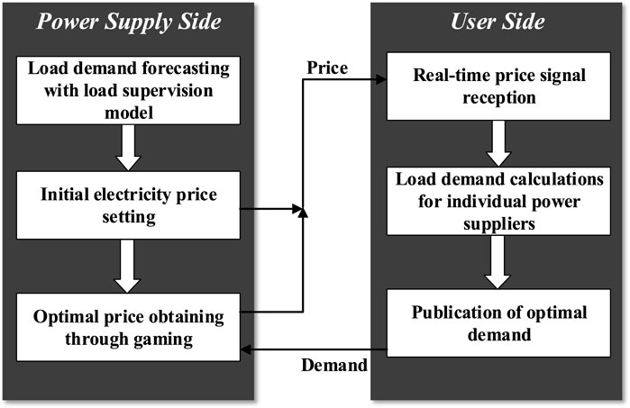
FIGURE 4. Game model.

Let ${\mathcal{S}}_{\mathcal{K}}$ and ${\mathcal{S}}_{\mathcal{N}}$ represent the strategy sets of power suppliers and users, respectively. For power suppliers, their strategy set mainly includes each power supplier’s price choice strategy, i.e., ${\mathcal{S}}_{\mathcal{K}}={\mathcal{S}}_1\times {\mathcal{S}}_2\times {\mathcal{S}}_3\times \cdots {\mathcal{S}}_K$. The users, being followers, have a strategy set that primarily passively responds to the price signals of power suppliers, i.e., ${\mathcal{S}}_{\mathcal{N}}={\mathcal{S}}_1\times {\mathcal{S}}_2\times {\mathcal{S}}_3\times \cdots {\mathcal{S}}_N$. Therefore, when the price competition among power suppliers reaches a Nash equilibrium, each power supplier’s price signal $p_k^{\star }$ satisfies:

$U_k\left(p_k^{\star },p_{-k}^{\star },d\left({\mathit{p}}^{\star }\right)\right)\ge U_k\left(p_k,p_{-k},d\left(\mathit{p}\right)\right)(37)$

where d(p^⋆) represents the users’ best response to the power suppliers’ prices. As users are only responding passively, there exists a unique best response to the price signals of power suppliers; i.e., the users’ optimal response signals are calculated through Eq. 22.

Thus, it only needs to be proven that a unique equilibrium point exists in the price competition among power suppliers. When power suppliers compete in price, they mainly consider their utility function U_k(p_k), which is a continuous concave function for any power supplier. This utility function, within a specified range, necessarily satisfies ${\partial }^2{U}_k/\partial p_k^2<0$. When ∂U_k/∂p_k = 0, the obtained price signal can ensure that the power supplier’s utility function has a unique maximum point within the specified range, and this signal satisfies $p_k^{\star }\in {\mathcal{S}}_{\mathcal{K}}={\mathcal{S}}_1\times {\mathcal{S}}_2\times {\mathcal{S}}_3\times \cdots {\mathcal{S}}_K$. Therefore, this proves the uniqueness of the Nash equilibrium in the price competition among power suppliers.

6 Simulations

6.1 Experiment of user load data prediction

6.1.1 Dataset

The data used for training the load supervision model come from a publicly available load dataset provided by MIT. This dataset captures the household load data of multiple users from 10 July 2014 to 31 December 2016. The data were collected through smart meter devices, with samples taken every 15 min, and include twelve features, such as temperature, humidity, pressure, wind speed, and perceived temperature of the environment, as well as the current load consumption data of multiple users. The load data of the users are shown in Figure 5.

FIGURE 5

FIGURE 5. Load data for users: (A) user 1; (B) user 2.

6.1.2 Simulation of load supervision model parameters

In deep learning networks, it is challenging to determine the number of hidden layers and the number of neurons in each layer. There is no strict theoretical way of determining the optimal numbers of hidden layers and neurons in a network structure. Before determining the number of hidden layers, it should be understood that the role of the hidden layers is mainly to increase the non-linear fitting ability of the model. If the input data are linearly separable, then hidden layers are not necessary. However, for more complex sequential and speech data, it may be necessary to add more hidden layers to improve the model’s learning capability. Once the number of hidden layers has been determined, the most important issue is how to determine the number of neurons in each layer. If there are too few neurons in the hidden layer, it will cause underfitting. If there are too many neurons, it may lead to overfitting. Therefore, selecting an appropriate number of neurons is extremely important.

This paper determines the relationship between the prediction accuracy and training time of the model with different numbers of layers and neurons through experiments, as shown in Figure 6.

FIGURE 6

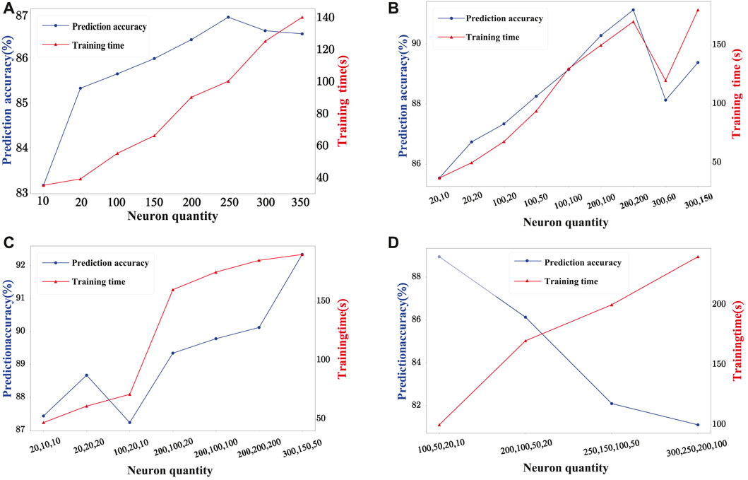
FIGURE 6. Impact of neuron quantity on prediction accuracy: (A) single-layer neural network; (B) two-layer neural network; (C) three-layer neural network; (D) four-layer neural network.

Figure 6 show that when using a three-layer neural network, the average prediction accuracy is the highest, and the average training time of the model is relatively low. When a four-layer neural network is used, the model enters a state of overfitting, results in the low overall prediction accuracy and the long training time. Besides, we can also observe from Figure 6 that the best prediction accuracy can be achieved when the numbers of neurons in each layer are (300, 150, 50).

6.1.3 Prediction results of user load

To speed up the model’s training time, the dataset is sampled every 30 min, reducing the scale of the training data. The overall flow of the training algorithm is to first divide the dataset that has not yet been trained into training, validation, and testing sets. Then, we set the number of layers and the number of neurons in each layer in the LSTM network of the load supervision model based on the model parameters from the previous subsection. Meanwhile, a dropout layer is added between each pair of layers to prevent overfitting. Finally, we specify the loss function for model training. Time series data delay steps of 1, 3, 5, 7, 10, and 15 days were selected for the load data prediction of user 1 and user 2. The delay step length refers to how many days of data are used to predict future load data. The longer the delay step length of the time series data, the more features will be obtained in the training data, allowing the model to better learn user behavior patterns. The results of user load data prediction are shown in Table 2.

TABLE 2

TABLE 2. User forecast accuracy.

For user 1, the highest prediction accuracy was achieved with a 10-day time series step delay, reaching 91.54%, higher than the 91.11% accuracy obtained with a 15-day time series step delay. The analysis shows that when training the model with a 15-day time series step delay, the number of features is significantly higher than that with a 10-day time series step delay. The trained prediction model should have a higher accuracy, but possibly because there are too many features, overfitting occurs, thus reducing the prediction accuracy on the test set. This can be prevented by setting the coefficient of the dropout layer, thereby improving the prediction accuracy of the model. For user 2, the highest prediction accuracy was achieved with a 15-day time series step delay, reaching 96.37%, and a lower prediction accuracy of 94.56% was achieved with a 7-day time series step delay. This indicates a significant difference in the power usage habits of user 2 on weekdays and weekends, resulting in a surge in load demand on the weekend and many jump points, thereby reducing the overall prediction accuracy. Generally, the LSTM-based load supervision model can achieve good prediction accuracy for future load demand.

6.2 Simulation and analysis of the demand response model

The optimization effect of the entire game model is studied by changing the user’s own electricity budget. In the experiment, the constant coefficients in the utility functions of all users are initially set to γ_n = 5, β_n = 5. Then, 10 users and 4 suppliers are considered in the demand response model, with the electricity budgets for the users are set as B₁ = 10, B₂ = 15, B₃ = 18, B₄ = 20, B₅ = 25, B₆ = 28, B₇ = 35, B₈ = 40, B₉ = 45, B₁₀ = 50. The capacities of the suppliers at each moment are set as G₁ = 10, G₂ = 15, G₃ = 20, G₄ = 30. After predicting the future load demand of each user based on the load supervision model, the initial electricity prices of the suppliers are set as p₁ = 1.5, p₂ = 2.2, p₃ = 2.5, p₄ = 2.0.

Figure 7A represents the optimal electricity prices set by each power supplier after the game as user 1’s electricity budget continues to increase. As the user’s budget increases, the electricity prices set by each power supplier also increase. Because Power Supplier 1 has the least capacity, the real-time electricity price it sets is the highest. Figure 7B represents the demand curves for electricity for each user. As user 1’s electricity budget continues to increase, the purchased electricity also increases. Since the production capacity of all suppliers is fixed at any moment, this leads to a decrease in the energy demand of other users, manifested as a declining trend in their demand curves. Figure 7C shows the profit curve of each power supplier. From this figure, it can be seen that the income of the power suppliers does not show a positive correlation with the real-time set electricity price. In the electricity price curve, the price set by Power Supplier 1 is the highest, but its profit is the lowest among all suppliers. In contrast, Power Supplier 4, which sets the lowest price, obtains the highest profit due to its larger capacity. Figure 7D represents the utility function curves of users. Since user 1 purchased a large amount of electricity, their utility curve gradually increases, causing the utility curves of other users to decrease, which conforms to real-life scenarios.

FIGURE 7

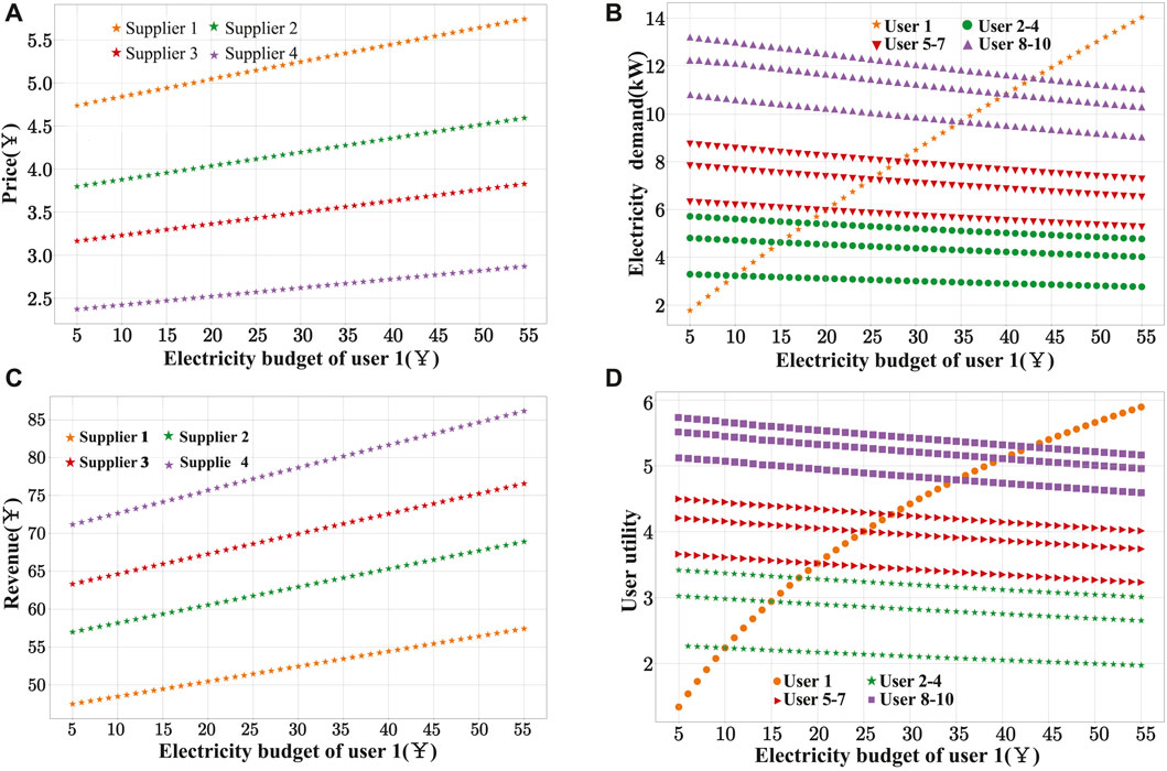
FIGURE 7. Optimization results of the game model: (A) power supplier price; (B) user demand; (C) power supplier revenue; (D) user utility.

To verify whether the introduction of a large-capacity power supplier will affect the utility of users, Power Supplier 5 was added to the original experiment, and its power supply capacity was set as G₅ = 100. Comparing Figure 8B and Figure 7D, it can be seen that when Power Supplier 5 is added, the utility of the users increases, indicating that the addition of Power Supplier 5 does not reduce the utility of the users. As shown in Figure 8A, it is almost impossible for a power supplier in the proposed game model to control prices by significantly increasing capacity; this will only lead to an overall excess capacity in the system, causing a decrease in the prices set by all power suppliers. Therefore, in the entire system model, the more capacity a power supplier has, the more the users’ utility will increase.

FIGURE 8

FIGURE 8. Optimization results of the game model after adding power supplier 5: (A) power supplier price; (B) user utility.

Finally, to further verify the application of the model in actual production, an analysis of user load data revealed that the load demand curves of all users exhibit a distinct regularity, reaching a peak at noon, followed by reduced consumption and an increase again in the evening. Therefore, we extracted a day’s energy consumption data and real-time electricity price information from the U.S. National Energy website. The dataset includes 2,000 users and 5 power suppliers. The energy consumption data of these users are used to verify whether the model can improve the utility of users. Figure 9 represents the energy consumption data of users at different times of the day. Figure 10 represents the prices set by the power suppliers after the game and the normal electricity prices set daily. Figure 11 shows that after adopting the real-time electricity prices calculated based on the game model, the overall expenditure of users decreases by 30% compared with traditional pricing model, indicating that when all power suppliers adopt real-time electricity prices calculated based on the game model, every user in the demand response model will gain substantial benefits.

FIGURE 9

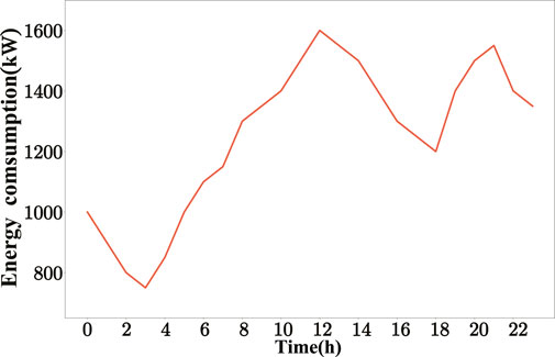
FIGURE 9. Energy consumption curves.

FIGURE 10

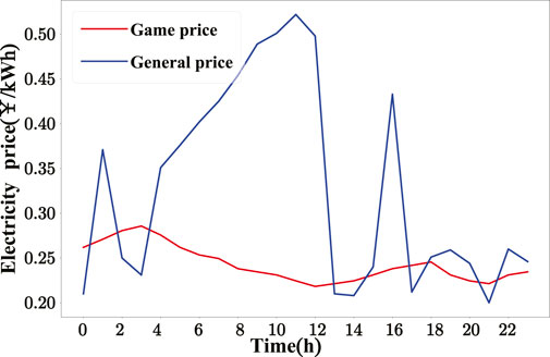
FIGURE 10. Real-time electricity price curves.

FIGURE 11

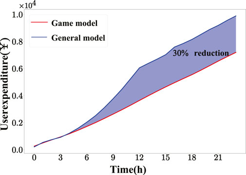
FIGURE 11. User expenditure curves.

7 Conclusion

In this paper, we employ a long short-term memory (LSTM) network as a load forecasting model to predict user load data in a smart grid and utilize a Stackelberg game model based on the load forecasting model to reduce the overall expenditure of energy users. The main contribution of this paper can be summarized as follows:

1) This paper employs an LSTM network as a load supervision model to forecast users’ load data. The LSTM network integrates gate structures and memory units internally, enabling it to memorize historical data effectively and predict users’ cyclical demand behaviors.

2) Based on the load supervision model, this paper built a Stackelberg game model to optimize the optimal power prices set by the power supplier in real time at each moment, making the demand response between users and the power supplier more efficient. Specifically, the power supplier first sets the initial power prices according to the forecasted user demand and then adjusts its power prices in real time in response to user reactions and price competition with other power suppliers, achieving its maximum profit.

3) This paper compares the prediction accuracy of forecasting models with different layers and numbers of neurons through simulation experiments and obtains optimal model parameters. Results of comparing actual user data and the prediction output demonstrate that LSTM-based load forecasting model achieves an accuracy of up to 96.37%. Additionally, the game model reduces the overall expenditure of users by 30% compared with the general pricing model.

Data availability statement

The original contributions presented in the study are included in the article/Supplementary Material, further inquiries can be directed to the corresponding author.

Author contributions

FC contributed to the conception, performed the experiment and wrote the manuscript. DA contributed to the manuscript correction and foundation support. GZ helped perform the analysis with constructive discussions. All authors contributed to the article and approved the submitted version.

Funding

This work was supported in part by the National Natural Science Foundation of China under Grant Nos. 62173268, 61803295, 61973247, and 61673315; in part by the Major Research Plan of the National Natural Science Foundation of China under Grant 61833015; in part by the National Postdoctoral Innovative Talents Support Program of China under Grant BX20200272; in part the National Key Research and Development Program of China under Grant 2019YFB1704103; and in part by the China Postdoctoral Science Foundation under Grant 2018M643659.

Conflict of interest

The authors declare that the research was conducted in the absence of any commercial or financial relationships that could be construed as a potential conflict of interest.

Publisher’s note

All claims expressed in this article are solely those of the authors and do not necessarily represent those of their affiliated organizations, or those of the publisher, the editors and the reviewers. Any product that may be evaluated in this article, or claim that may be made by its manufacturer, is not guaranteed or endorsed by the publisher.

References

Abubakar, I., Khalid, S., Mustafa, M., Shareef, H., and Mustapha, M. (2017). Application of load monitoring in appliances’ energy management–a review. Renew. Sustain. Energy Rev. 67, 235–245. doi:10.1016/j.rser.2016.09.064

CrossRef Full Text | Google Scholar

Afrasiabi, M., Mohammadi, M., Rastegar, M., Stankovic, L., Afrasiabi, S., and Khazaei, M. (2020). Deep-based conditional probability density function forecasting of residential loads. IEEE Trans. Smart Grid 11, 3646–3657. doi:10.1109/tsg.2020.2972513

CrossRef Full Text | Google Scholar

Alhmoud, L., and Nawafleh, Q. (2021). Short-term load forecasting for Jordan power system based on narx-elman neural network and arma model. IEEE Can. J. Electr. Comput. Eng. 44, 356–363. doi:10.1109/icjece.2021.3076124

CrossRef Full Text | Google Scholar

Bokkisam, H. R., Singh, S., Acharya, R. M., and Selvan, M. P. (2022). Blockchain-based peer-to-peer transactive energy system for community microgrid with demand response management. CSEE J. Power Energy Syst. 8, 198–211. doi:10.17775/CSEEJPES.2020.06660

CrossRef Full Text | Google Scholar

Cai, T., Wu, C., and Zhang, J. (2022). “A bagging long short-term memory network for financial transmission rights forecasting,” in 2022 7th IEEE workshop on the electronic grid (eGRID) (IEEE), 1–5.

CrossRef Full Text | Google Scholar

Chen, C., Lu, N., Jiang, B., Xing, Y., and Zhu, Z. H. (2021). Prediction interval estimation of aeroengine remaining useful life based on bidirectional long short-term memory network. IEEE Trans. Instrum. Meas. 70, 1–13. doi:10.1109/tim.2021.3126006

PubMed Abstract | CrossRef Full Text | Google Scholar

Cheng, L., Chen, Y., and Liu, G. (2022). 2pns-eg: a general two-population n-strategy evolutionary game for strategic long-term bidding in a deregulated market under different market clearing mechanisms. Int. J. Electr. Power Energy Syst. 142, 108182. doi:10.1016/j.ijepes.2022.108182

CrossRef Full Text | Google Scholar

Cheng, L., and Yu, T. (2019). Game-theoretic approaches applied to transactions in the open and ever-growing electricity markets from the perspective of power demand response: an overview. IEEE Access 7, 25727–25762. doi:10.1109/access.2019.2900356

CrossRef Full Text | Google Scholar

Gao, Y., Ma, J., Wang, J., and Wu, Y. (2023). Event-triggered adaptive fixed-time secure control for nonlinear cyber-physical system with false data-injection attacks. IEEE Trans. Circuits Syst. II Express Briefs 70, 316–320. doi:10.1109/tcsii.2022.3217823

CrossRef Full Text | Google Scholar

Gellings, C. W., Samotyj, M., and Howe, B. (2004). The future’s smart delivery system [electric power supply]. IEEE Power Energy Mag. 2, 40–48. doi:10.1109/mpae.2004.1338121

CrossRef Full Text | Google Scholar

Gyamfi, S., Krumdieck, S., and Urmee, T. (2013). Residential peak electricity demand response—Highlights of some behavioural issues. Renew. Sustain. Energy Rev. 25, 71–77. doi:10.1016/j.rser.2013.04.006

CrossRef Full Text | Google Scholar

Hermias, J. P., Teknomo, K., and Monje, J. C. N. (2017). “Short-term stochastic load forecasting using autoregressive integrated moving average models and hidden markov model,” in 2017 international conference on information and communication technologies (ICICT) (IEEE), 131–137.)

CrossRef Full Text | Google Scholar

Huang, S.-J., and Shih, K.-R. (2003). Short-term load forecasting via arma model identification including non-Gaussian process considerations. IEEE Trans. power Syst. 18, 673–679. doi:10.1109/tpwrs.2003.811010

CrossRef Full Text | Google Scholar

Jasim, A. M., Jasim, B. H., Flah, A., Bolshev, V., and Mihet-Popa, L. (2023). A new optimized demand management system for smart grid-based residential buildings adopting renewable and storage energies. Energy Rep. 9, 4018–4035. doi:10.1016/j.egyr.2023.03.038

CrossRef Full Text | Google Scholar

Khan, M. A., Saleh, A. M., Waseem, M., and Sajjad, I. A. (2023). Artificial intelligence enabled demand response: prospects and challenges in smart grid environment. IEEE Access 11, 1477–1505. doi:10.1109/access.2022.3231444

CrossRef Full Text | Google Scholar

Liu, N., Yu, X., Wang, C., Li, C., Ma, L., and Lei, J. (2017). Energy-sharing model with price-based demand response for microgrids of peer-to-peer prosumers. IEEE Trans. Power Syst. 32, 3569–3583. doi:10.1109/tpwrs.2017.2649558

CrossRef Full Text | Google Scholar

Mahela, O. P., Khosravy, M., Gupta, N., Khan, B., Alhelou, H. H., Mahla, R., et al. (2022). Comprehensive overview of multi-agent systems for controlling smart grids. CSEE J. Power Energy Syst. 8, 115–131. doi:10.17775/CSEEJPES.2020.03390

CrossRef Full Text | Google Scholar

Mansouri, S. A., Paredes, Ángel, González, J. M., and Aguado, J. A. (2023). A three-layer game theoretic-based strategy for optimal scheduling of microgrids by leveraging a dynamic demand response program designer to unlock the potential of smart buildings and electric vehicle fleets. Appl. Energy 347, 121440. doi:10.1016/j.apenergy.2023.121440

CrossRef Full Text | Google Scholar

Mocanu, E., Nguyen, P. H., Gibescu, M., and Kling, W. L. (2016). Deep learning for estimating building energy consumption. Sustain. Energy, Grids Netw. 6, 91–99. doi:10.1016/j.segan.2016.02.005

CrossRef Full Text | Google Scholar

Orlando, M., Estebsari, A., Pons, E., Pau, M., Quer, S., Poncino, M., et al. (2022). A smart meter infrastructure for smart grid iot applications. IEEE Internet Things J. 9, 12529–12541. doi:10.1109/jiot.2021.3137596

CrossRef Full Text | Google Scholar

Panda, S., Mohanty, S., Rout, P. K., Sahu, B. K., Parida, S. M., Kotb, H., et al. (2022). An insight into the integration of distributed energy resources and energy storage systems with smart distribution networks using demand-side management. Appl. Sci. 12, 8914. doi:10.3390/app12178914

CrossRef Full Text | Google Scholar

Sivasankarareddy, V., Sundari, G., Rami Reddy, C., Aymen, F., and Bortoni, E. C. (2021). Grid-based routing model for energy efficient and secure data transmission in wsn for smart building applications. Appl. Sci. 11, 10517. doi:10.3390/app112210517

CrossRef Full Text | Google Scholar

Sofana Reka, S., and Ramesh, V. (2016). A demand response modeling for residential consumers in smart grid environment using game theory based energy scheduling algorithm. Ain Shams Eng. J. 7, 835–845. doi:10.1016/j.asej.2015.12.004

CrossRef Full Text | Google Scholar

Tang, R., Wang, S., and Li, H. (2019). Game theory based interactive demand side management responding to dynamic pricing in price-based demand response of smart grids. Appl. Energy 250, 118–130. doi:10.1016/j.apenergy.2019.04.177

CrossRef Full Text | Google Scholar

Trujillo, D., and García Torres, E. M. (2022). Demand response due to the penetration of electric vehicles in a microgrid through stochastic optimization. IEEE Lat. Am. Trans. 20, 651–658. doi:10.1109/tla.2022.9675471

CrossRef Full Text | Google Scholar

Walther, J., Spanier, D., Panten, N., and Abele, E. (2019). Very short-term load forecasting on factory level–a machine learning approach. Procedia CIRP 80, 705–710. doi:10.1016/j.procir.2019.01.060

CrossRef Full Text | Google Scholar

Wang, L., Hou, C., Ye, B., Wang, X., Yin, C., and Cong, H. (2021). Optimal operation analysis of integrated community energy system considering the uncertainty of demand response. IEEE Trans. Power Syst. 36, 3681–3691. doi:10.1109/tpwrs.2021.3051720

CrossRef Full Text | Google Scholar

Wang, L., Jones, D., Chapman, G. J., Siddle, H. J., Russell, D. A., Alazmani, A., et al. (2020). A review of wearable sensor systems to monitor plantar loading in the assessment of diabetic foot ulcers. IEEE Trans. Biomed. Eng. 67, 1989–2004. doi:10.1109/tbme.2019.2953630

PubMed Abstract | CrossRef Full Text | Google Scholar

Zhang, Z., Huang, Y., Chen, Z., and Lee, W.-J. (2023). Integrated demand response for microgrids with incentive compatible bidding mechanism. IEEE Trans. Industry Appl. 59, 118–127. doi:10.1109/tia.2022.3204626

CrossRef Full Text | Google Scholar

Zheng, S., Sun, Y., Qi, B., and Li, B. (2022). Incentive-based integrated demand response considering S&amp;C effect in demand side with incomplete information. IEEE Trans. Smart Grid 13, 4465–4482. doi:10.1109/tsg.2022.3149959

CrossRef Full Text | Google Scholar