
95% of researchers rate our articles as excellent or good
Learn more about the work of our research integrity team to safeguard the quality of each article we publish.
Find out more
ORIGINAL RESEARCH article
Front. Energy Res. , 29 September 2023
Sec. Process and Energy Systems Engineering
Volume 11 - 2023 | https://doi.org/10.3389/fenrg.2023.1234624
 Mohammed A. Saeed1,2
 El-Sayed M. El-Kenawy3*
 Abdelhameed Ibrahim4
 Abdelaziz A. Abdelhamid5,6
 Marwa M. Eid7
 Faten Khalid Karim8*
 Doaa Sami Khafaga8
 Laith Abualigah9,10,11,12,13,14,15
It is difficult to analyze and anticipate the power output of Combined Cycle Power Plants (CCPPs) when considering operational thermal variables such as ambient pressure, vacuum, relative humidity, and temperature. Our data visualization study shows strong non-linearity in the experimental data. We observe that CCPP energy production increases linearly with temperature but not pressure. We offer the Waterwheel Plant Algorithm (WWPA), a unique metaheuristic optimization method, to fine-tune Recurrent Neural Network hyperparameters to improve prediction accuracy. A robust mathematical model for energy production prediction is built and validated using anticipated and experimental data residuals. The residuals’ uniformity above and below the regression line suggests acceptable prediction errors. Our mathematical model has an R-squared value of 0.935 and 0.999 during training and testing, demonstrating its outstanding predictive accuracy. This research provides an accurate way to forecast CCPP energy output, which could improve operational efficiency and resource utilization in these power plants.
Electricity is the lifeblood of modern civilization and one of the most important building blocks of human progress on every continent. A massive quantity of electricity is needed to keep our economy and society running smoothly. As a result of the increasing need for electricity, combined cycle power plants (CCPP) are being utilized in an increasing number of locations around the world (Ganjehkaviri et al., 2015). The CCPP is a huge power plant that combines gas turbines and steam turbines to produce electricity. They make use of fossil fuels to attain the highest possible level of technical efficiency in power generation, which has now been shown to be greater than 0.60 (Kotowicz and Brzęczek, 2018). Atmospheric pressure, relative humidity, exhaust pressure, and outside air temperature are the four most important factors in a power plant’s basic load functioning, all of which affect the amount of electricity produced (Tüfekci, 2014). The system’s power output could be affected by small adjustments to these variables. Thermodynamic methods are typically utilized in thermal power plants as a means of conducting precise system analyses in preparation for the operation of the plant. This method relies on a large number of numerical assumptions and parameters in order to answer the thousands of non-linear equations that need to be solved. The explanation of these equations either requires an excessive amount of effort and time to compute, or it is sometimes difficult to solve these equations without the use of these numerical assumptions (Kesgin and Heperkan, 2005). In place of thermodynamic methodologies and mathematical modeling, machine learning (ML) techniques are being employed to examine systems for unpredictable output and input (Shuvo et al., 2021).
Some of the many ML models developed for the many existing challenges have received more attention than others because of their greater adaptability to non-linear simulations (Khafaga et al., 2022; Alhussan et al., 2022). An ANNs model takes into account both environmental factors and nonlinear interactions, with the generated power serving as an output. One of these promising approaches is artificial neural networks (ANNs). With the help of an ANN model, we can determine the plant’s output power under different scenarios.
Based on the information collected from the power plant and using the ANN model described in Kesgin and Heperkan (2005), various effects on the power plant, such as relative humidity, ambient pressure, and ambient temperature, are analyzed. The performance and operational characteristics of a gas turbine are calculated using an ANN model (Fast et al., 2009), which takes into account the changing local air conditions. Researchers evaluated and contrasted a variety of ML approaches (Siddiqui et al., 2021) to compute the full load output of electrical power generated by a CCPP that was operating on base load. In the study presented by Rahnama et al. (2012), an artificial neural network system is developed and employed to model stationary gas turbines. The ANN system proves to be effective in examining the behavior of gas turbines across various operating conditions, ranging from full-speed full load to no-load situations. Furthermore, in Refan et al. (2012), researchers successfully utilize radial basis function (RBF) and multi-layer perception (MLP) networks to identify the start-up stage of a stationary gas turbine. Lorencin et al. (2019) estimated the CCPP’s electrical power production and performance using MLP models with varying solvers, hidden layer topologies, and activation functions. The authors (Yari et al. 2013) compare the performance of feed-forward neural networks (FFNNs) and dynamic linear models for the identification of gas turbines. The study reveals that neural networks, specifically FFNNs, outperform dynamic linear models in terms of prognostication, showcasing superior performance and accuracy. The authors conclude that neural networks serve as a more effective model for predicting and analyzing the behavior of gas turbines compared to traditional linear models. ANN models have proven to be highly effective in various applications related to gas turbine engines. In addition to the mentioned uses, ANNs are successfully employed in isolation, fault detection, anomaly detection, and performance analysis of gas turbine engines, as highlighted in Tayarani-Bathaie et al. (2014). This study demonstrated the versatility and reliability of ANN models in addressing important aspects such as identifying faults, detecting anomalies, and analyzing the performance of gas turbine engines. Using FFNNs, which are entirely based on a novel trained particle swarm optimization method, the authors (Elfaki and Ahmed, 2018) anticipated the total electrical energy power output of the CCPP. They calculated the hourly average power output of the CCPP by using atmospheric pressure, relative humidity, vacuum, and ambient temperature as input inputs. A machine learning (ML) processing tool based on artificial neural networks is employed with a predictive approach (Roni and Khan, 2017). The study focuses on CCPPs and utilizes the ANN-based ML tool to investigate and analyze the environmental impact on CCPP generation. By leveraging the predictive capabilities of ANNs, the researchers can assess and understand how various environmental factors affect the operation and performance of CCPPs. This approach provides valuable insights into the environmental implications of CCPP generation and can assist in developing strategies for optimizing their environmental impact. Numerous studies (Tso and Yau, 2007; Azadeh et al., 2010; Che et al., 2012; Leung and Lee, 2013) have been conducted in the literature to predict electrical energy consumption using machine learning intelligence tools. However, there are relatively fewer studies that specifically focus on calculating the overall electrical power of a CCPP with a heating system consisting of one steam turbine and three gas turbines. The authors (Xu and Yan, 2019) employ an extreme learning machine (ELM) as the underlying regression model to analyze the performance of the power plant under varying environmental conditions. The ELM model is designed to autonomously update regression models to adapt to sudden or gradual changes in the environment. This approach allows for a more robust analysis of the power plant’s performance in dynamic atmospheric conditions. Furthermore, (Chatterjee et al., 2018), utilize a Cuckoo Search-based ANN to predict the output electrical energy of a gas turbine and combined steam mechanisms. This integration of Cuckoo Search optimization with ANN aims to enhance the reliability and accuracy of the prediction models for these energy-generating systems. The author (Heydari et al., 2020) predicts the price of electricity and the demand for power of CCPP using a combination of a gravitational search optimization algorithm and a compound neural network. The author picks the input data by using feature selection. The culmination of the simulations demonstrates the improved accuracy and consistency of the new model. Guo et al. (2006) utilized support vector regression to make predictions regarding the power output of combined cycle power plants and proved its suitability for this purpose.
Based on the research cited above, it appears that artificial intelligence has contributed novel understanding to the study of characteristics related to combined cycle power plants, especially with regard to power efficiency predictions. This method of prediction, which is based on CCPP features, is important for the long-term development of power plants. Accuracy is crucial in complex engineering processes like these and improving it can lead to significant benefits in terms of cost and time.
This paper is organized as follows; In Section 2, we describe the CCPP system, which is the starting point for the work that will be done to make predictions based on CCPP data. The materials and methods proposed in this manuscript are discussed in Section 3. In section 4, we explain the proposed methodology. Our findings from mathematical modeling, data visualization, RNN, and WWPA modeling are presented in Section 5. Section 6 concludes with some final thoughts.
A combined cycle power plant is a type of electricity generator that combines two distinct thermodynamic cycles. It’s made to make the most efficient use of fuel by incorporating both gas and steam turbines.
Steam turbines, heat recovery steam generators (HRSG), and gas turbines are the main three components that make up a combined cycle power plant as shown in Figure 1. The procedure starts with a gas turbine, which is very much like a jet engine in its operation. The turbine can be used to burn natural gas or another gaseous fuel, which results in the generation of gas that is both extremely hot and extremely pressurized. This causes the gas to expand, which in turn powers the blades of the turbine, which are connected to a generator to produce energy. The gas that is expelled from the gas turbine still retains a sizeable portion of its original thermal energy. The gas turbine’s high-temperature exhaust is piped to a heat-recovery steam generator. The HRSG takes the gas turbine’s exhaust heat and turns it into usable steam. Water running through tubes absorbs heat from the exhaust gas, creating high-pressure steam. After being created in the HRSG, the high-pressure steam is subsequently fed into a steam turbine to be used as the driving force. When the steam expands and moves through the blades of the steam turbine, it transfers its kinetic energy to the turbine, which is then connected to another generator to produce extra power (Ibrahim et al., 2017).
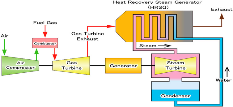
FIGURE 1. Combined cycle power plant schematic diagram.
Combined cycle power plants offer several advantages:
• The utilization of both gas and steam cycles enables the generation of electricity at a significantly better overall efficiency. This, in turn, results in less consumption of fuel and fewer emissions of greenhouse gases.
• Gas turbines have a rapid starting capability, which enables them to provide rapid response times to changes in the energy demand. Because of their adaptability, combined cycle power plants are appropriate for the generation of both baseload and peak-load electricity.
• The recovery of waste heat, which is accomplished with the help of the HRSG, makes the plant more efficient and has less negative impact on the environment.
• CHP Potential The capability of combined cycle power plants to generate both usable heat and electricity makes them ideally suited for cogeneration applications, which in turn improves the efficiency with which energy is used overall.
This section provides the research principles and approaches of this study, concentrating primarily on the mathematical formulae and models applied in the RNN and WPA algorithms. This was done so that the introduction of improved algorithms in the subsequent section would be easier.
The data collection contains 9,568 points of information that were gathered from a combined cycle power plant (UCI, 2014) during a period of 6 years (2006–2011), during which time the plant was configured to operate at full load. The plant consists of one 160 MW ABB steam turbine, two dual-pressure heat recovery steam generators, and two 160 MW ABB 13E2 gas turbines. It is considered to have a modest 480 MW producing capacity.
The selection process for the dataset involved the following: In the first stage, a feature relevance analysis was conducted to ascertain the variables that are most likely to have an impact on the electrical power output of a CCPP. To discover pairings of variables that had a strong link, a correlation analysis was undertaken. The implementation of this approach effectively mitigated the potential problems associated with multicollinearity in our model (El-Kenawy et al., 2022a). After selecting pertinent and uncorrelated factors, we systematically created all conceivable combinations of these variables, taking into account various input configurations that may impact the power output of the CCPP system. To choose the final subsets, we employed performance measurements obtained from preliminary tests, including mean squared error and R-squared values (Hassib et al., 2019). These metrics were utilized to identify the combinations that resulted in the most optimal dataset which contains 15 distinct combinations of five variables.
The following values are calculated using data collected from a network of sensors spread across the plant; temperature (AT) between 1.81°C and 37.11°C, pressure (AP) between 992.89 and 1033.30 millibars, relative humidity (RH) between 25.56% and 100.16%, An exhaust vacuum (V) between 25.36 and 81.56 millibars, hourly power (PE) output of 420.26–495.76 MW Net. To get useful insights from data, preprocessing is an essential step that uses various methods (El-kenawy et al., 2022b). Emptying the dataset of missing or null values is a standard preparation procedure. Null values can introduce bias into analysis and produce erroneous results. Removing these variables can improve the data quality and guarantee accurate insights (Abdelhamid et al., 2022). Normalization, particularly the min-max normalization approach, is a crucial preprocessing technique. Data is typically scaled between 0 and 1 when using this method (Eid and Zaki, 2022). When working with variables that have varied scales or units, normalization is a must (Khafaga, 2022). To avoid any one variable dominating the study due to its scale alone, we rescale the data to bring them within a common range, allowing for direct comparison. Figure 2 shows a scatter plot that proves the closeness of the results of the actual and predicted features.
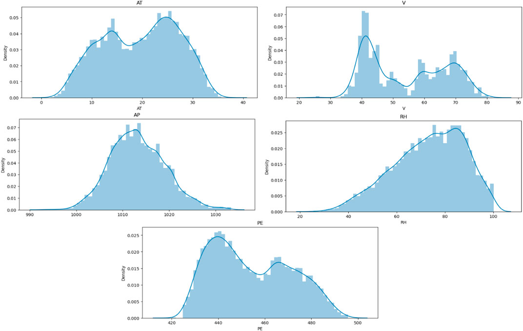
FIGURE 2. Scatter plot of the actual and predicted features.
Figure 3 shows the correlation matrix which is a useful statistical tool for analyzing the bond between the variables in the dataset. It often forms a matrix and displays the pairwise correlations between all variables (Hassan et al., 2022). The correlation coefficients, which can range from −1 to +1, show the relationships’ relative strength and direction (Takieldeen et al., 2022). We may examine the data’s dependencies, patterns, and potential predictors by using a correlation matrix to see which variables are positively or negatively correlated. This knowledge is useful for predictive modeling since it aids in feature selection, dimensionality reduction, and the detection of multicollinearity problems (El-kenawy et al., 2022c). The selection of 15 distinct combinations of variables for the following reasons:
a. Our objective was to guarantee that the chosen combinations effectively encompass a diverse array of input circumstances that the CCPP system may experience in practical applications. The presence of variability inside our model contributes to its ability to generalize effectively (El-kenawy et al., 2022d).
b. In order to encompass all pertinent variables identified in the analysis of feature relevance, the 15 combinations were deliberately chosen. This methodology enables the assessment of the influence of individual variables on the generation of power (Oubelaid et al., 2023).
c. The assessment of the robustness of our predictive model can be achieved by conducting tests on various combinations. This aids in the identification of variables that consistently exert influence and those that may exhibit effects particular to certain contexts (Towfek, 2023).
d. The inclusion of a collection of 15 unique combinations enables us to conduct a comparative analysis of our model’s performance across a diverse range of scenarios, facilitating the derivation of more comprehensive and robust conclusions regarding its efficacy (Towfek et, 2023).

FIGURE 3. A correlation matrix.
It is an innovative form of stochastic optimization that is inspired by the workings of natural systems proposed by Abdelhamid (2022). Modeling the natural behavior of the waterwheel plant when it is on a hunt is the foundation of the fundamental idea behind the WWPA that has been developed. The strategy that waterwheel plants employ to identify their insect prey, trap it, and then relocate it to a more accessible area before consuming it served as the primary source of inspiration for the fundamental notion of WWPA (Alkattan H et al., 2023; Alhasani et al., 2023). In the following section, we will discuss the ideas that led to the creation of the algorithm, as well as the mathematical model for its technique.
The Waterwheel plant, also known as Aldrovanda vesiculosa, possesses small transparent flytrap-like structures on its broad petiole. These traps, measuring approximately 1/12 inch, are safeguarded from harm or accidental activation by surrounding bristle-like hairs. Similar to the teeth of a flytrap, the trap’s outer edges are covered in hook-shaped teeth that interlock when the trap closes around its prey. Inside the trap, around forty elongated trigger hairs, comparable to the trigger hairs found in Venus’s flytraps, are responsible for triggering the closure of the trap. Predators also possess acid-secreting glands to aid in digestion. Once ensnared, the unfortunate victim is sealed by the trap’s interlocking teeth and a mucus sealant, effectively trapping it and guiding it toward the base of the trap near the hinge. The majority of the prey’s nutrients are absorbed as the trap digests the remaining water. Each Aldrovanda trap can capture and consume two to four meals before becoming inactive, much like a flytrap. Figure 4 depicts an image of the waterwheel plant.
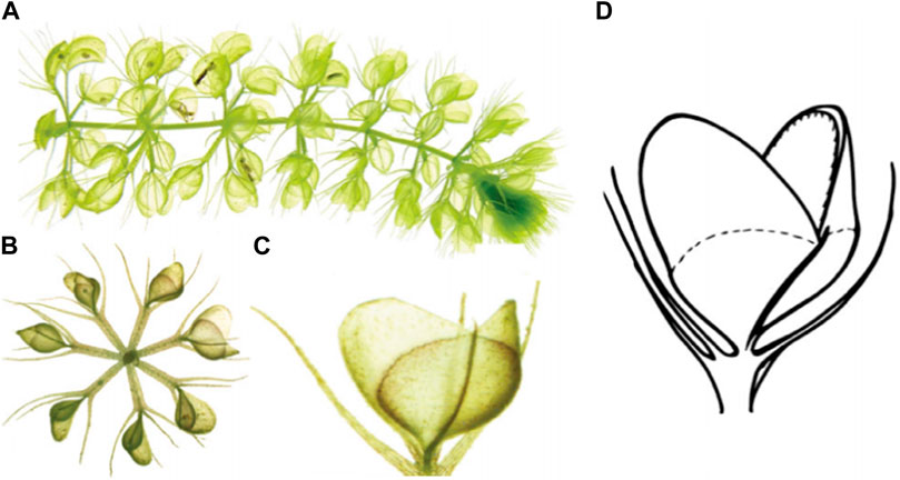
FIGURE 4. Waterwheel Plant Image. (A) Lateral view on a free-floating shoot with numerous traps. (B) Frontal view with open and closed traps. (C) Single open trap. (D) Schematic drawing of an open trap.
The WWPA is a population-based method that uses iteration to find an appropriate solution based on its population members’ search capacity in the universe of possible solutions. The WWPA population waterwheels have problem variable values based on their search space position. Thus, each waterwheel represents a vector-based solution. A matrix Eq. 1 represents the WWPA population of waterwheels. WWPA initializes waterwheel positions in the search space randomly using Eq. 2.
In this context, N represents the number of waterwheels, while m indicates the number of variables. The value
Every waterwheel is considered as a possible solution to the problem, and thus, the objective function can be evaluated for each one of them. Previous research has demonstrated that a vector can be employed to efficiently represent the values that form the objective function of the problem.
F is a vector containing all objective function values, and
Waterwheels possess a strong predatory instinct thanks to their highly developed sense of smell, enabling them to effectively track and locate pests. When an insect enters the waterwheel’s vicinity, it initiates an attack and pursues the target by accurately identifying its position. The WWPA (Waterwheel Predator Algorithm) employs a simulation of this hunting behavior to model the initial phase of its population updating process. By incorporating the waterwheel’s attack on the insect, the WWPA enhances its ability to explore the optimal region and avoid getting trapped in local optima. Consequently, significant positional shifts occur within the search space as a result of this modeling. To determine the new location of the waterwheel, an equation is employed in conjunction with the simulation of the waterwheel’s approach toward the insect. If relocating the waterwheel to this new position leads to an increase in the value of the goal function, the previous location is abandoned in favor of the newly described one.
If the solution fails to improve for three consecutive iterations, the position of the waterwheel can be altered using the following equation.
In this context, the variables
The second step of population update in WWPA mimics the behavior of waterwheels capturing and transporting insects to a feeding tube. This simulated behavior is utilized to enhance the exploitation capability of WWPA during local search, enabling the algorithm to converge towards better solutions that are close to previously discovered ones. By modeling the process of transporting the insect to the appropriate tube, slight changes are introduced to the waterwheel’s position within the search space. For each waterwheel in the population, WWPA’s designers initially determine a new random location referred to as a “good position for consuming insects,” emulating the natural activity of waterwheels. Subsequently, if the goal function value is higher at this new location, the waterwheel is moved to this new position, replacing the previous location, as described by the following equations.
In this scenario,
where F and C are independent random variables with values between (−5, 5). Furthermore, the following equation can be used to demonstrate the exponential decay of K:
The WWPA is offered as a procedure that can be repeated. Adjusting the positions of all waterwheels is the final step in implementing WWPA after the first two stages have been carried out.
After comparing target function values, the optimal solution candidate is improved. For the next iteration, the waterwheels’ positions are adjusted, and so on, until the algorithm reaches its ultimate iteration. The steps necessary to implement WWPA are laid down in pseudocode form in Algorithm 1. After a sufficient number of iterations, WWPA presents the best possible candidate answer it has been storing.
Algorithm 1.The proposed WWPA algorithm.
1: Initialize the positions
2: Calculate the fitness of
3: Find the best plant position
4: Set t = 1.
5: while t ≤ Tmax do
6: for (i = 1: i<n+1) do
7: if (r < 0.5) then
8: Explore the search space of waterwheel plants using:
9: if the solution does not change for three iterations, then
10: end if
11: else
12: Exploit the current solutions to obtain the best solution using:
13: if the solution does not change for three iterations, then
14: end if
15: end if
16: end for
17: Decrease the value of K exponentially using:
18: Update r,
19: Calculate the objective function
20: Find the best position
21: Set t = t + 1.
22: end while
23: Return the best solution
Tuning parameters in recurrent neural networks can benefit significantly from WWPA. To get the most out of an RNN and make the most accurate predictions possible, tuning its parameters is essential. To use WWPA for adjusting parameters in RNNs, we must first determine which parameters should be optimized. Some examples of hyperparameters that can be changed to modify the network’s behavior are the learning rate, the number of hidden units, the batch size, and the like. WWPA uses the fact that the most robust Waterwheel Plant typically finds the best spot in nature. The technique begins by creating a pool of solutions for different parameter settings. Each key, or Waterwheel Plant, is given a fitness value based on how well it performs on a validation set.
Waterwheel Plants are moved throughout the search space to find optimal solutions. WWPA employs weighted vectors to direct Waterwheel Plants to suitable areas. The Waterwheel Plants’ fitness ratings are used to calculate these vectors. The algorithm constantly adjusts the Waterwheel Plants’ locations to reflect the greatest possible outcome. WWPA attempts to converge on the best possible RNN parameter configuration by iteratively refining the solutions. The algorithm terminates after a fixed number of iterations or upon reaching a convergence threshold (Abdelhamid et al., 2023b), at which point the optimal solution is chosen; in this case, the parameter configuration with the highest fitness value.
Recurrent Neural Networks (RNNs) are a subcategory of artificial neural networks that were developed to process sequential input through the use of feedback connections. In contrast to feedforward neural networks, which process data in only one way from input to output, RNNs can keep internal memory, which enables them to remember information about prior inputs even as they process new ones. In the 1980s, RNNs were developed. However, its widespread implementation occurred until recently (Salehinejad et al., 2018). Increases in computer power, especially the efficiency of parallel processing units on graphics cards, have been a driving factor in RNNs’ development. Time series forecasting (including electrical load forecasting, weather forecasting, stock market forecasting, etc.) is just one of the many modern applications for recurrent neural networks. Since RNNs are dynamic systems, their internal state changes at each classification time step. This occurs because neurons in different layers can communicate with one another via self-feedback and recurrent connections. Data from previous occurrences can be fed into the RNN’s current processing steps via these feedback connections. Thus, RNNs learn to remember past occurrences in a time series. In sequential data, RNNs may detect temporal dependencies and context. An RNN’s neuron takes input from both the current time step and its previous state, forming a loop that preserves information. The network may handle arbitrary sequential data with this recurrent connection.
Figure 5 illustrates the arrangement and relationships within a basic recurrent neural network during both forward and backward propagation. Xi represents the input at time step i, si denotes the state of the recurrent cell at time step i, and
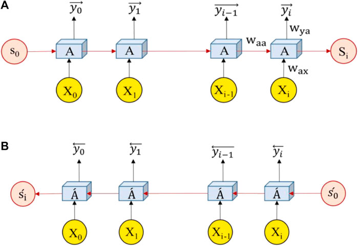
FIGURE 5. RNN forward and backward propagation. (A) Forward propagation (B) Backward propagation.
Where,
In order to determine the output at time step i, we use the softmax activation function. In order to generate a probability distribution over numerous classes, the softmax function is frequently employed in machine learning and deep learning. It takes a vector as input, multiplies each element by an exponent, and then divides the resulting values by the sum of the exponents to achieve normalization. By using this normalization, we can guarantee that the resulting values are all interpretable probabilities and fall inside the range (0, 1).
Where, i = 1,2, , k,
The vanishing gradient problem is an obstacle in RNN training because it makes it harder to capture long-term dependencies since gradients decrease exponentially when they are backpropagated in time (Yu et al., 2019). The authors propose using Long Short-Term Memory (LSTM) networks, which have gating mechanisms to regulate the gradient and information flows, to solve this problem. The steps necessary to implement RNN are laid down in pseudocode form in Algorithm 2.
Algorithm 2.The proposed RNN algorithm.
A. Initialize Parameters:
1. Initialize the weights and biases of the RNN layers randomly or using a specific initialization technique.
2. Set the learning rate, the number of epochs, and other hyperparameters.
3. Define the Activation Function
4. Choose an activation function suitable for the problem, such as the hyperbolic tangent (tanh) or sigmoid function.
B. Forward Pass
5. Compute the hidden state at the current time step by applying the activation function to the linear combination of the input and previous hidden state.
6. Compute the output of the RNN by applying a linear transformation (dot product) to the hidden state.
7. Store the hidden state and output for each time step.
C. Compute Loss
8. Compare the predicted outputs of the RNN with the ground truth targets using a suitable loss function, such as mean squared error (MSE) or cross-entropy loss.
D. Backward Pass (Backpropagation Through Time)
9. Initialize the gradients of the parameters with zeros.
10. Compute the gradient of the output layer concerning the loss.
11. Backpropagate the gradient through the RNN layer to obtain the gradient of the hidden state.
12. Update the gradients of the parameters using the computed gradients and the input at the current time step.
13. Accumulate the gradients of the hidden state from the previous time step.
E. Update Parameters
14. Update the weights and biases of the RNN using the WWPA optimization algorithm.
15. Adjust the parameters based on the computed gradients and the learning rate.
F. Repeat
16. Repeat steps B to E for the specified number of epochs or until convergence.
G. Prediction
17. After training, the RNN can be used for prediction by feeding new input sequences and propagating them through the trained network.
18. Apply the forward pass steps described in step B to compute the predicted outputs.
Extensive testing is carried out in order to provide evidence of the efficacy and superiority of the proposed WWPA algorithm. In the trials, Windows 10 and Python 3.9 are utilized, both of which are run at 3.00 GHz on an Intel(R) Core (TM) i5 processor. (Manufacturer: Intel Corporation, located in California, United States). Experiments were carried out in the context of a case study, and the findings involved a comparison of the output of the RNN-WWPA approach to that of baseline models’ output on a dataset consisting of information about power output prediction from CCPP. The configuration settings of both the WWPA and other optimization approaches are displayed in Table 1.
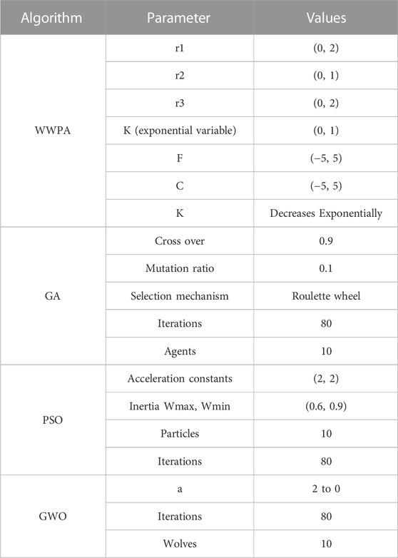
TABLE 1. Configuration parameters of the WWPA and competing optimization algorithms.
In this section, we will conduct an analysis and evaluation of the strategy that has been suggested for CCPP output prediction. The evaluation is carried out with the help of the proposed algorithm for feature selection and the proposed model that is WWPA-based optimized. The results that were recorded will be presented together with a description according to three stages.
Additional measures are employed to evaluate the performance of regression models used for predicting output power in a combined cycle power plant. These metrics include root mean squared error (RMSE), mean absolute error (MAE), mean bias error (MBE), Pearson’s correlation coefficient (r), coefficient of determination (R2), relative root mean squared error (RRMSE), Nash Sutcliffe Efficiency (NSE), and agreement determination (WI). Here, “N” represents the total number of observations in the dataset,
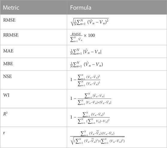
TABLE 2. Prediction evaluation criteria (Abdelhamid et al., 2023a).
Table 3 presents a comparison between the various models’ respective performance metrics. According to the findings, the proposed WWPA-RNN model gave the best root mean squared error with 0.13%, so the proposed model has a lower level of error or discrepancy between its predictions and the actual data points. The proposed WWPA-RNN model’s predictions have a low relative error of 61.23% compared to the range or variability of the target variable. It indicates that the model’s predictions are relatively accurate and have a lower level of discrepancy compared to the spread of the data. The squared error for the proposed model is close to 1 so, the independent variables in the model have a strong relationship with the dependent variable and are effective in explaining the variability in the data. The proposed model proves its efficiency and accuracy as the NSE value near 1 indicates that the model captures the underlying processes or relationships accurately and performs exceptionally well in reproducing the observed data.
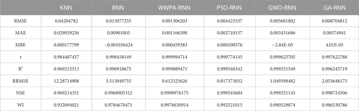
TABLE 3. Comparison of the performance metrics for different models.
The previous stage results provide further evidence of the viability of the strategy that was recommended. In addition, the results of the predictions are subjected to statistical examination, the findings of which are shown in Table 4. The outcomes of the statistical analysis are compared with those of the other seven optimization algorithms in the following table. The findings of the research and the comparison demonstrate that the proposed model is preferable.
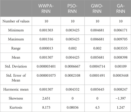
TABLE 4. Statistical analysis of the prediction results achieved by the proposed WWPA-RNN model.
Several tests were conducted to evaluate the statistical significance of the optimized stacked ensemble. The statistical procedures included both the Wilcoxon signed-rank test and the ANOVA test. The results of these tests can be found in Tables 5, 6. Table 5 shows that the p-value for the proposed method is less than 0.0001, indicating a statistical difference between the proposed method and the other techniques tested. Furthermore, the p-value for the proposed method is lower than the p-value for the other methods used in the experiments. Similarly, Table 6 also confirms the statistical difference and significance of the suggested approach, with the recorded p-value supporting its significance.
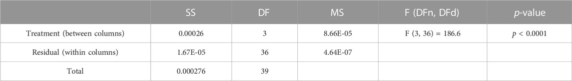
TABLE 5. ANOVA test applied to the prediction results achieved by the proposed WWPA-RNN model.
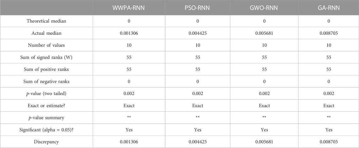
TABLE 6. Wilcoxon test applied the prediction results achieved by the proposed WWPA-RNN model.
In order to enhance the performance and interpretability of machine learning models, a significant emphasis is placed on quantitative evaluation, data-driven decision-making, dimensionality reduction, and model interpretation. These aspects, facilitated by statistical techniques, are crucial for selecting relevant features and improving model performance. To examine the effectiveness of the two feature selection methods, we employ a one-way analysis of variance (ANOVA) test to determine if there exists a statistically significant difference between them.
Feature selection often employs analysis of variance (ANOVA) as a widely used technique. Its primary purpose is to assess the statistical significance of multiple features concerning the target variable. By analyzing the mean values of the target variable across different levels or categories of a feature, ANOVA helps uncover the relationship between each feature and the objective variable. The calculation involves an F-statistic, which measures the ratio of variance between group means to the variance within groups. A higher F-statistic indicates greater differences between the means of the compared groups, suggesting that the feature being evaluated may hold greater importance in predicting the target variable.
Visual analysis of the generated power from the CCPP is conducted using the plots displayed in Figure 6. These plots, including residual, homoscedasticity, quartile-quartile (QQ), and heatmap, provide insight into the performance of the proposed method in predicting power output. The plots demonstrate that the proposed method shows promising results in predicting the generated power. Specifically, the residual and homoscedasticity plots indicate minimal prediction errors when estimating power output from the combined cycle power plant. Additionally, the QQ and heatmap plots suggest robust prediction capabilities.
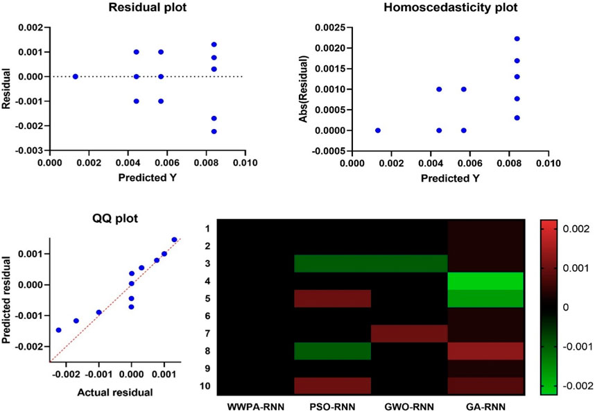
FIGURE 6. Visualizing the results of CCPP predicted output power.
Figures 7, 8 show the accuracy values obtained by the suggested technique in comparison to the other three methods and the histogram, respectively. Figure 7 shows the accuracy values provided by the suggested methodology. This comparison was carried out so that the resilience of the suggested optimized model could be illustrated in a way that was simple enough to be comprehended by everyone. The fact that the method that was presented was able to achieve the greatest possible accuracy value is evidence that the method is both reliable and resilient.
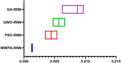
FIGURE 7. Visualizing accuracy comparison values of the proposed WWPA-RNN optimization algorithm and other competitive ones.
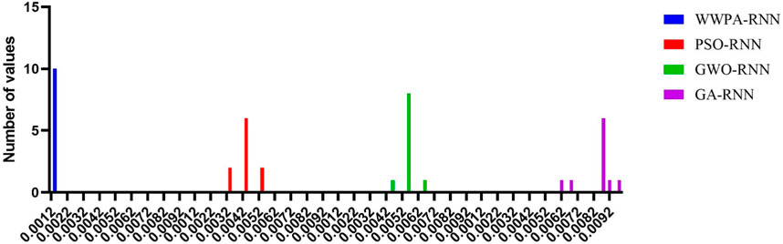
FIGURE 8. Histogram of the accuracy values for the proposed WWPA-RNN optimization algorithm and other competitive ones.
Finally, the significance and implications of accurate electrical power output prediction for combined cycle power plants may be discussed as follows.
By making real-time adjustments to factors like fuel consumption, turbine speed, and inlet air conditions based on accurate predictions of electrical power generation, CCPPs may maximize their efficiency. As a result of this optimization, energy production efficiency is improved, with fewer resources being squandered, and more electricity being produced. CCPPs can optimize fuel consumption through accurate power output forecasts. As a result, both fuel use and operational costs have decreased. Predictive models can be used to anticipate when equipment may break or its performance may degrade, allowing for preventative maintenance that lessens disruptions and saves money.
Emissions of greenhouse gases and other pollutants can be decreased if energy production is optimized as a consequence of accurate power output forecast. This is consistent with environmental sustainability objectives and regulatory mandates. Better integration of CCPPs into the electricity grid is possible with more precise projections. Electricity supply can be better planned and managed by grid operators, leading to greater system stability and reliability.
The results of this study have implications for CCPPs’ long-term strategy as well as their day-to-day operations. Owners and operators of power plants can utilize the information to make informed decisions about capital enhancements and new initiatives. Data-driven operations allow CCPPs to utilize predictive models for continual process optimization. More flexible and responsive power plants may be the result of this transition. The study’s findings provide CCPP operators with immediate, actionable insights into power output.
In order to anticipate the electrical power output of a CCPP running at base load, this study provided an alternate solution model. Machine learning methods were selected for accurate prediction in place of thermodynamic methods, which rely on assumptions and have intractably many nonlinear equations of a real-world application of a system. Thermodynamic approaches to system analysis are computationally intensive and may produce incorrect results due to the substantial number of assumptions made and the complexity of the resulting non-linear equations. To get around this problem, several machine-learning regression approaches were given for forecasting the output of a thermodynamic system—specifically, a combined-cycle power plant with two gas turbines, one steam turbine, and two heating systems. Finding out which type of machine learning regression was the most accurate in predicting full-load electrical power output is the primary objective of this research. All of the available subsets of the dataset, which contain 15 distinct combinations of five variables AT, V, AP, PE, and RH, were subjected to a total of two distinct machine-learning regression methods and four hybrid algorithms. The WWPA-RNN approach was determined to be the most successful approach, which might forecast the full load electrical power output of a base load operated CCPP with the maximum prediction accuracy, according to the average findings of the comparative trials. The CCPP from which the data was taken can rely on the proposed method to predict the different variables through which the amount of energy produced from this plant can be calculated.
The original contributions presented in the study are included in the article/Supplementary Material, further inquiries can be directed to the corresponding authors.
Conceptualization, E-SE-K; methodology, MS and E-SE-K; software, E-SE-K and AI; validation ME formal analysis, FK, LA, and DK; investigation, E-SE-K and AI; writing–original draft, MS, E-SE-K, and ME; writing–review and editing AI, LA, and E-SE-K; visualization, ME, FK, and DK; project administration, E-SE-K. All authors contributed to the article and approved the submitted version.
Princess Nourah Bint Abdulrahman University Researchers Supporting Project number (PNURSP2023R300), Princess Nourah Bint Abdulrahman University, Riyadh, Saudi Arabia.
The authors declare that the research was conducted in the absence of any commercial or financial relationships that could be construed as a potential conflict of interest.
All claims expressed in this article are solely those of the authors and do not necessarily represent those of their affiliated organizations, or those of the publisher, the editors and the reviewers. Any product that may be evaluated in this article, or claim that may be made by its manufacturer, is not guaranteed or endorsed by the publisher.
Abdelhamid, A. A., El-Kenawy, E. S. M., Khodadadi, N., Mirjalili, S., Khafaga, D. S., Alharbi, A. H., et al. (2022). Classification of monkeypox images based on transfer learning and the Al-Biruni Earth Radius Optimization algorithm. Mathematics 10 (19), 3614. doi:10.3390/math10193614
Abdelhamid, A. A., Eid, M. M., Abotaleb, M., and Towfek, S. K. (2023b). Identification of cardiovascular disease risk factors among diabetes patients using ontological data mining techniques. J. Artif. Intell. Metaheuristics 4 (2), 45–53. doi:10.54216/JAIM.040205
Abdelhamid, A. A. (2022). Machine learning-based model for talented students identification. J. Artif. Intell. Metaheuristics 1 (2), 31–41. doi:10.54216/JAIM.010204
Abdelhamid, A. A., Towfek, S. K., Khodadadi, N., Alhussan, A. A., Khafaga, D. S., Eid, M. M., et al. (2023a). Waterwheel plant algorithm: A novel metaheuristic optimization method. Processes 11 (5), 1502. doi:10.3390/pr11051502
Alhasani, A. T., Alkattan, H., Subhi, A. A., El-Kenawy, E. S. M., and Eid, M. M. (2023). A comparative analysis of methods for detecting and diagnosing breast cancer based on data mining. Methods 7, 9. doi:10.54216/JAIM.040201
Alhussan, A. A., Khafaga, D. S., El-Kenawy, E. S. M., Ibrahim, A., Eid, M. M., and Abdelhamid, A. A. (2022). Pothole and plain road classification using adaptive mutation dipper throated optimization and transfer learning for self driving cars. IEEE Access 10, 84188–84211. doi:10.1109/ACCESS.2022.3196660
Alkattan, H., Towfek, S. K., and Shams, M. Y. (2023). Tapping into knowledge: ontological data mining approach for detecting cardiovascular disease risk causes among diabetes patients. J. Artif. Intell. Metaheuristics 4 (1), 08–15. doi:10.54216/JAIM.040101
Azadeh, A., Saberi, M., and Seraj, O. (2010). An integrated fuzzy regression algorithm for energy consumption estimation with non-stationary data: A case study of Iran. Energy 35 (6), 2351–2366. doi:10.1016/j.energy.2009.12.023
Chatterjee, S., Dey, N., Ashour, A. S., and Drugarin, C. V. A. (2018). “Electrical energy output prediction using cuckoo search based artificial neural network,” in Smart trends in systems, security and sustainability: Proceedings of WS4 2017 (Singapore: Springer), 277–285.
Che, J., Wang, J., and Wang, G. (2012). An adaptive fuzzy combination model based on self-organizing map and support vector regression for electric load forecasting. Energy 37 (1), 657–664. doi:10.1016/j.energy.2011.10.034
Eid, M. M., and Zaki, R. M. (2022). Classification of student performance based on ensemble optimized using dipper throated optimization. J. Artif. Intell. Metaheuristics 2 (1), 36–45. doi:10.54216/JAIM.020104
El-kenawy, E. S. M., Albalawi, F., Ward, S. A., Ghoneim, S. S., Eid, M. M., Abdelhamid, A. A., et al. (2022b). Feature selection and classification of transformer faults based on novel meta-heuristic algorithm. Mathematics 10 (17), 3144. doi:10.3390/math10173144
El-kenawy, E. S. M., Ibrahim, A., Bailek, N., Bouchouicha, K., Hassan, M. A., Jamei, M., et al. (2022c). Sunshine duration measurements and predictions in saharan Algeria region: an improved ensemble learning approach. Theor. Appl. Climatol. 147, 1015–1031. doi:10.1007/s00704-021-03843-2
El-kenawy, E. S. M., Ibrahim, A., Mirjalili, S., Zhang, Y., Elnazer, S., and Zaki, R. M. (2022d). Optimized ensemble algorithm for predicting metamaterial antenna parameters. Comput. Mater. Continua 71 (3), 4989–5003. doi:10.32604/cmc.2022.023884
El-Kenawy, E. S. M., Zerouali, B., Bailek, N., Bouchouich, K., Hassan, M. A., Almorox, J., et al. (2022a). Improved weighted ensemble learning for predicting the daily reference evapotranspiration under the semi-arid climate conditions. Environ. Sci. Pollut. Res. 29 (54), 81279–81299. doi:10.1007/s11356-022-21410-8
Elfaki, E. A., and Ahmed, A. H. (2018). Prediction of electrical output power of combined cycle power plant using regression ANN model. J. Power Energy Eng. 6 (12), 17–38. doi:10.4236/jpee.2018.612002
Eskandari, H., Imani, M., and Moghaddam, M. P. (2021). Convolutional and recurrent neural network based model for short-term load forecasting. Electr. Power Syst. Res. 195, 107173. doi:10.1016/j.epsr.2021.107173
Fast, M., Assadi, M., and De, S. (2009). Development and multi-utility of an ANN model for an industrial gas turbine. Appl. Energy 86 (1), 9–17. doi:10.1016/j.apenergy.2008.03.018
Ganjehkaviri, A., Jaafar, M. M., and Hosseini, S. E. (2015). Optimization and the effect of steam turbine outlet quality on the output power of a combined cycle power plant. Energy Convers. Manag. 89, 231–243. doi:10.1016/j.enconman.2014.09.042
Guo, X. C., Liang, Y. C., Wu, C. G., and Wang, H. Y. (2006). “Electric load forecasting using SVMS,” in 2006 International Conference on Machine Learning and Cybernetics, Dalian, China, 13-16 August 2006, 4213–4215. doi:10.1109/ICMLC.2006.258945
Hassan, M. A., Bailek, N., Bouchouicha, K., Ibrahim, A., Jamil, B., Kuriqi, A., et al. (2022). Evaluation of energy extraction of PV systems affected by environmental factors under real outdoor conditions. Theor. Appl. Climatol. 150 (1-2), 715–729. doi:10.1007/s00704-022-04166-6
Hassib, E. M., El-Desouky, A. I., El-Kenawy, E. S. M., and El-Ghamrawy, S. M. (2019). An imbalanced big data mining framework for improving optimization algorithms performance. IEEE Access 7, 170774–170795. doi:10.1109/ACCESS.2019.2955983
Heydari, A., Nezhad, M. M., Pirshayan, E., Garcia, D. A., Keynia, F., and De Santoli, L. (2020). Short-term electricity price and load forecasting in isolated power grids based on composite neural network and gravitational search optimization algorithm. Appl. Energy 277, 115503. doi:10.1016/j.apenergy.2020.115503
Ibrahim, K. T., Mohammed, M. K., Awad, O. I., Rahman, M. M., Najafi, G., Basrawi, F., et al. (2017). The optimum performance of the combined cycle power plant: A comprehensive review. Renew. Sustain. Energy Rev. 79, 459–474. doi:10.1016/j.rser.2017.05.060
Kesgin, U., and Heperkan, H. (2005). Simulation of thermodynamic systems using soft computing techniques. Int. J. energy Res. 29 (7), 581–611. doi:10.1002/er.1095
Khafaga, D. (2022). Meta-heuristics for feature selection and classification in diagnostic breast cancer. Comput. Mater. Continua 73 (1), 749–765. doi:10.32604/cmc.2022.029605
Khafaga, D. S., Alhussan, A. A., El-Kenawy, E. S. M., Ibrahim, A., Eid, M. M., and Abdelhamid, A. A. (2022). Solving optimization problems of metamaterial and double T-shape antennas using advanced meta-heuristics algorithms. IEEE Access 10, 74449–74471. doi:10.1109/ACCESS.2022.3190508
Kotowicz, J., and Brzęczek, M. (2018). Analysis of increasing efficiency of modern combined cycle power plant: A case study. Energy 153, 90–99. doi:10.1016/j.energy.2018.04.030
Leung, P. C., and Lee, E. W. (2013). Estimation of electrical power consumption in subway station design by intelligent approach. Appl. Energy 101, 634–643. doi:10.1016/j.apenergy.2012.07.017
Lorencin, I., Car, Z., Kudláček, J., Mrzljak, V., Anđelić, N., and Blažević, S. (2019). “Estimation of combined cycle power plant power output using multilayer perceptron variations,” in 10th International Technical Conference-Technological Forum, Prague: Czech, June 2019, 94–98.
Oubelaid, A., Ibrahim, A., and Elshewey, A. M. (2023). Bridging the gap: An explainable methodology for customer churn prediction in supply chain management. doi:10.54216/JAIM.040102
Rahnama, M., Ghorbani, H., and Montazeri, A. (2012). “Nonlinear identification of a gas turbine system in transient operation mode using neural network,” in The 4th Conference on Thermal Power Plants, Tehran, Iran, 18-19 December 2012, 1–6.
Refan, M. H., Taghavi, S. H., and Afshar, A. (2012). “Identification of heavy-duty gas turbine startup mode by neural networks,” in The 4th Conference on Thermal Power Plants, Tehran, Iran, 18-19 December 2012, 1–6.
Roni, M. H. K., and Khan, M. A. G. (2017). “An artificial neural network based predictive approach for analyzing environmental impact on combined cycle power plant generation,” in 2017 2nd International Conference on Electrical & Electronic Engineering (ICEEE), Rajshahi, Bangladesh, 27-29 December 2017, 1–4. doi:10.1109/CEEE.2017.8412913
Salehinejad, H., Sankar, S., Barfett, J., Colak, E., and Valaee, S. (2018). Recent advances in recurrent neural networks. arXiv preprint arXiv:1801.01078. Available at: https://arxiv.org/abs/1801.01078.
Shuvo, M. G. R., Sultana, N., Motin, L., and Islam, M. R. (2021). “Prediction of hourly total energy in combined cycle power plant using machine learning techniques,” in 2021 1st international conference on artificial intelligence and data analytics (CAIDA), Riyadh, Saudi Arabia, 06-07 April 2021, 170–175. doi:10.1109/CAIDA51941.2021.9425308
Siddiqui, R., Anwar, H., Ullah, F., Ullah, R., Rehman, M. A., Jan, N., et al. (2021). Power prediction of combined cycle power plant (CCPP) using machine learning algorithm-based paradigm. Wirel. Commun. Mob. Comput. 2021, 1–13. doi:10.1155/2021/9966395
Takieldeen, A. E., El-kenawy, E. S. M., Hadwan, M., and Zaki, R. M. (2022). Dipper throated optimization algorithm for unconstrained function and feature selection. Comput. Mater. Contin. 72, 1465–1481. doi:10.32604/cmc.2022.026026
Tayarani-Bathaie, S. S., Vanini, Z. S., and Khorasani, K. (2014). Dynamic neural network-based fault diagnosis of gas turbine engines. Neurocomputing 125, 153–165. doi:10.1016/j.neucom.2012.06.050
Towfek, S. K. (2023). A semantic approach for extracting the medical association rules. J. Artif. Intell. Metaheuristics 5 (1), 46–52. doi:10.54216/JAIM.050105
Towfek, S. K., khodadadi, E., and Talaat, F. M. (2023). Automated detection and segmentation of COVID-19 infection using machine learning. J. Artif. Intell. Metaheuristics 3 (2), 28–37. doi:10.54216/JAIM.030203
Tso, G. K., and Yau, K. K. (2007). Predicting electricity energy consumption: A comparison of regression analysis, decision tree and neural networks. Energy 32 (9), 1761–1768. doi:10.1016/j.energy.2006.11.010
Tüfekci, P. (2014). Prediction of full load electrical power output of a base load operated combined cycle power plant using machine learning methods. Int. J. Electr. Power & Energy Syst. 60, 126–140. doi:10.1016/j.ijepes.2014.02.027
UCI (2014). Machine learning repository. Available at: https://archive.ics.uci.edu/ml/datasets/combined+cycle+power+plant (Accessed September 6, 2023).
Xu, R., and Yan, W. (2019). “Continuous modeling of power plant performance with regularized extreme learning machine,” in 2019 International Joint Conference on Neural Networks (IJCNN), Budapest, Hungary, 14-19 July 2019, 1–8. doi:10.1109/IJCNN.2019.8852137
Yari, M., Shoorehdeli, M. A., and Yousefi, I. (2013). “V94. 2 gas turbine identification using neural network,” in 2013 First RSI/ISM International Conference on Robotics and Mechatronics (ICRoM), Tehran, Iran, 13-15 February 2013, 523–529. doi:10.1109/ICRoM.2013.6510160
Keywords: power plant, combined cycle, machine learning, energy output, neural networks, waterwheel plant algorithm
Citation: Saeed MA, El-Kenawy E-SM, Ibrahim A, Abdelhamid AA, Eid MM, Karim FK, Khafaga DS and Abualigah L (2023) Electrical power output prediction of combined cycle power plants using a recurrent neural network optimized by waterwheel plant algorithm. Front. Energy Res. 11:1234624. doi: 10.3389/fenrg.2023.1234624
Received: 05 June 2023; Accepted: 12 September 2023;
Published: 29 September 2023.
Edited by:
Xu Chen, Jiangsu University, ChinaReviewed by:
Shiqiang Jin, Bristol Myers Squibb, United StatesCopyright © 2023 Saeed, El-Kenawy, Ibrahim, Abdelhamid, Eid, Karim, Khafaga and Abualigah. This is an open-access article distributed under the terms of the Creative Commons Attribution License (CC BY). The use, distribution or reproduction in other forums is permitted, provided the original author(s) and the copyright owner(s) are credited and that the original publication in this journal is cited, in accordance with accepted academic practice. No use, distribution or reproduction is permitted which does not comply with these terms.
*Correspondence: El-Sayed M. El-Kenawy, c2tlbmF3eUBpZWVlLm9yZw==; Faten Khalid Karim, ZmtkaWFhbGRpbkBwbnUuZWR1LnNh
Disclaimer: All claims expressed in this article are solely those of the authors and do not necessarily represent those of their affiliated organizations, or those of the publisher, the editors and the reviewers. Any product that may be evaluated in this article or claim that may be made by its manufacturer is not guaranteed or endorsed by the publisher.
Research integrity at Frontiers
Learn more about the work of our research integrity team to safeguard the quality of each article we publish.