Online correction of the transient voltage security region boundary based on load parameter variations in power systems

The transient voltage security region (TVSR) is an essential part of the dynamic safety region of a power system, which represents the safe operating region of the transient voltage where there is no loss in stability. The power system load significantly affects the transient voltage stability. However, the load model in the existing power systems, which considers the security region of the dynamic process, is too simple to comprehensively characterize the load characteristics of the dynamic process. Furthermore, it neglects the influence of the load model parameters on the dynamic process security region. In this study, a composite load model with distributed photovoltaic power is used as the research object. The main load parameters affecting the voltage stability and the generator nodes that are sensitive to the load parameters are calculated using the trajectory sensitivity method. The TVSR of the system is constructed based on the load and generator’s active powers. The correlations between different load-leading parameter combination scenarios and TVSR boundary points are mined using the CatBoost learning framework. Thus, the TVSR boundary can be promptly corrected online based on the changes in the load parameters, and the system security boundary can be described more accurately. The proposed method is verified using the IEEE39 and IEEE118 node systems. It is observed that the proposed method can correct the TVSR boundary online with high precision corresponding to real-time changes in the load model parameters. This provides a more accurate TVSR boundary for the power system operation scheduler, which helps in guiding it to control the system more accurately.

1 Introduction

The power load is the core of power consumption and significantly affects the design, analysis, and control of power systems (Arif et al., 2018). The complexity, time variability, and randomness of power system loads are constantly increasing with the development of the social economy, and the load exhibits more diverse dynamic characteristics. Therefore, it is essential to establish a load model that is as close as possible to the actual load characteristics for simulation calculation and to perform a more accurate simulation analysis of a power system. In load modeling at high-voltage levels, the load models are primarily divided into two categories: static and dynamic load models. The static load model includes the constant impedance, constant current, and constant power load models (IEEE Standards Association, 2020). The dynamic load model includes an induction motor (Arif et al., 2018). In recent years, an increasing number of distributed power sources have been connected to the grid, owing to the development of emerging smart grid technologies, such as distributed generators. Access to distributed power significantly affects the load characteristics (Song and Blaabjerg, 2017). Mather (2012) established a distributed photovoltaic cell model with grid-connected inverters to simulate the characteristics of distributed photovoltaics similar to a constant power load. Soliman et al. (1997) proposed an AND dynamic equivalent model, which considers static load, dynamic load, and distributed generation. In this paper, we comprehensively analyze the applicability of a load model and adopt the composite load model with distributed photovoltaic power as the research object. Following the selection of the appropriate load model, the parameters of the load model must be determined according to the actual regional load operation characteristics. Two main types of load model parameter identification methods are commonly used: component-based modeling (Gaikwad et al., 2016; Zhu et al., 2012) and measurement-based modeling (Hu et al., 2016; Visconti et al., 2014). The component-based modeling method has limitations due to the requirement of acquiring massive amounts of data. Therefore, modeling methods based on measurement data are preferable and widely implemented. Consequently, extensive research has been conducted on the application of modeling methods based on measurement data. In Han et al. (2009), Rodríguez-García et al. (2020), and Avila et al. (2020), an equivalent load model was established based on the measured data on the load under a large disturbance of the system, and the model parameters were identified. In Wang et al. (2022), the load model parameters online were identified based on the measurement data on the load during routine operation.

The power system security region is an area that ensures the safe and stable operation of the power system. Any operating point within the security region of the power system is considered safe. Conversely, any operating point outside the security region of a power system is considered unsafe (Yixin et al., 2020). The power system security region includes the power flow, static, small disturbances, and dynamic security region (Yixin et al., 2020). Here, the dynamic security region is the region in the power injection space before an expected accident, which ensures the transient stability of the system after the accident, and its boundary can be fitted by using one or more hyperplanes (Yixin et al., 2020). This region primarily focuses on the generator power angle and bus voltage during the dynamic process of the power system. The dynamic security theory of a power system overcomes the limitations to the running state of the system. It corresponds only to the system network structure and parameters before and after an expected accident (Yuan and Yu, 2002). The dynamic security theory has been implemented in several fields of power systems. In the study by Zeng et al. (2006), the effective application of the dynamic security theory in power systems is described. Zhang et al. (2017) presented a practical solution for dynamic security regions based on the coupling correlation of the system power flow. Maihemuti et al. (2021) solved the problem of a dynamic security region of an integrated energy system with natural gas access through high renewable energy permeability. In the study by Zhou et al. (2018), the transient stability of the access nodes on wind farms was analyzed by constructing a dynamic security region. Finally, Xiran et al. (2013) proposed a power system emergency control strategy based on a dynamic security region.

The load is the most variable component of the power system; it has the most significant effect on the safety and stability of the system and largely determines the process of voltage collapse (Li et al., 2006; Meng et al., 2014; Monteiro Pereira et al., 2008). However, several accidents have occurred in recent years involving power system stability problems caused by changes in load characteristics. For example, the power-grid voltage collapse incident in Tokyo, Japan (July 1987), was caused by the dynamic characteristics of a sudden and substantial increase in temperature control loads. Therefore, an accurate load model is crucial for analyzing power system security and stability (Taylor, 1994). With the development of load modeling technology, particularly online load identification technology, it has become possible to analyze load characteristics in real-time. Changes in the power system network parameters caused by variations in the load model or load parameters lead to a change in the dynamic security region of the power system. Therefore, it is necessary to closely monitor changes in the dynamic security region under the load model, load parameters, and load power changes. It is complicated and computationally expensive to analyze the safety and stability of each running state using the point-by-point method for load power that fluctuates frequently. However, using the security region to describe the safe operating boundary of the load significantly reduces the number of calculations and presents considerable potential for engineering applications. Therefore, the influence of real-time load changes on the dynamic security-region boundary must be comprehensively analyzed. Furthermore, the dynamic security-region boundary can be modified in real time to more accurately represent the dynamic security-region changes of the system and provide a valuable reference for power system schedulers.

In previous studies, a constant power load model was used in the calculation for the construction and analysis of the dynamic security region of a power system, with the dynamic characteristics of the load ignored. Therefore, we have considered a composite load model with distributed photovoltaic power as the research object in this study to overcome the existing issues. The load-dominant parameters that significantly affect the system voltage in the load model were calculated through sensitivity analysis. The key generator nodes were sensitive to the load parameters, with the load power changes calculated through a trajectory sensitivity analysis. The transient voltage security region (TVSR) was constructed using the active generator and load powers, and the TVSR boundary characteristics under different load–voltage-dominant parameters were analyzed. A fast TVSR boundary correction method under load-parameter changes was proposed based on the CatBoost learning framework. The online modification of the TVSR boundary can be realized based on changes in the load parameters through offline training of the TVSR boundary points in the scenario of multiple load parameters. The proposed method was verified using the IEEE39 and IEEE118 node systems.

Based on the increasing proportion of distributed power supply units in power systems, the proposed TVSR online correction method can realize real-time correction of the TVSR boundary due to changes in the load model parameters containing the distributed power supply. This provides a more accurate TVSR boundary for the operation scheduler to guide the operation scheduler in conducting more precise system operation regulations.

2 Transient voltage security region of power systems

2.1 Correlation between the transient voltage stability and injected power of system nodes

Transient voltage instability is primarily attributed to the transient failure or misoperation of the system, which causes a voltage drop in the system node and leads to a voltage collapse of the entire system. When a transient fault occurs in the system, the voltage at the short-circuit point is zero, and the other nodes in the system exhibit corresponding voltage drops based on the strength of the connection to the short-circuit point. A part of the electromagnetic power is lost due to the transient failure of the system, and the mechanical power of the prime mover surpasses the electromagnetic power. Thus, the prime mover continues to accelerate, leading to a further decline in the system voltage, causing transient voltage instability.

The node injection active power and reactive power significantly affect the transient process of the power system (Yu et al., 2006). The active power injected into the nodes mutates due to the occurrence of transient faults, leading to a system power imbalance and fluctuations in the dynamic components of the system, which further results in transient fluctuations in the system voltage and frequency. Conversely, the reactive power injected by the nodes causes the voltage of the power system to fluctuate temporarily when a transient fault occurs. The nodes with reactive power support ability adjust their reactive power to stabilize the node voltage to suppress these voltage fluctuations. For example, a generator excitation system adjusts the excitation current to stabilize the generator node voltage when it experiences a transient fault.

In the dispatching operation of an actual power system, the operation controller controls the output of the active power of the generator and the power consumption of the active power of the load. Essentially, the operation controller controls the active power injected by the node. Therefore, we focus primarily on the active power injection of the system nodes for power system operation and dispatching controllers. Furthermore, in high-voltage power networks, it is assumed that the reactive power of the nodes can be balanced locally. Therefore, in this study, we analyzed the effect of node active power injection on the transient process of the system, particularly on the transient voltage. In future studies, a sufficient reactive power reserve will be provided for the generator nodes of the system, and an analysis will be conducted on the correlation between the active power injection of the nodes and the transient voltage stability.

When the system load increases and more power is required from the generator, the node injection power increases along with the output of the generator excitation system. Accordingly, the dynamic response ability of the system decreases, which leads to the weakening of the voltage maintenance ability of the system when the transient fault occurs. Thus, increasing the node-injected power decreases the transient voltage stability of the system, making it essential to analyze the stability of the transient voltage of a power system based on the node-injection power.

2.2 Definition of the transient voltage security region

The power system security region of the dynamic process was defined in the node power injection space before the accident. This is the set of all the operating points that can maintain the transient stability after experiencing a large disturbance. For a specific accident, the structure of the power system goes through three stages, that is, before, during, and after the accident, and the corresponding equation of state is given as follows:

$\dot{\mathit{x}}=\left\{\begin{array}{l}{\mathit{f}}_{\mathit{i}}\left(\mathit{x}\right)-\mathit{\infty }<\mathit{t}<\mathbf{0},\\ {\mathit{f}}_{\mathit{F}}\left(\mathit{x}\right)\mathbf{0}\le \mathit{t}<\mathit{\tau },\\ {\mathit{f}}_{\mathit{j}}\left(\mathit{x}\right)\mathit{\tau }\le \mathit{t}<+\mathit{\infty },\end{array}\right.(1)$

where $\mathit{x}$ denotes the state variable of the system and $\mathit{\tau }$ denotes the duration of the accident. ${\mathit{f}}_{\mathit{i}}$, ${\mathit{f}}_{\mathit{F}}$, and ${\mathit{f}}_{\mathit{j}}$ represent the equations of the state of the system before, during, and after an accident, respectively.

The dynamic security region in the injection space can be expressed as follows:

${\mathit{\Omega }}_{\mathit{d}}\left(\mathit{i},\mathit{j},\mathit{\tau }\right)=\left\{\mathit{y}\left|{\mathit{x}}_{\mathit{d}}\left(\mathit{y}\right)\in \mathit{A}\left(\mathit{y}\right)\right.\right\},(2)$

where $\mathit{y}$ denotes the node power injection vector of the system, ${\mathit{x}}_{\mathit{d}}\left(\mathit{y}\right)$ denotes the state of the system at the time of accident clearing, and $\mathit{A}\left(\mathit{y}\right)$ denotes the stable region of the stable equilibrium point in the state space of the system after failure, which is determined by the injection, $\mathit{y}$. The boundary of the dynamic security domain can be represented by ${\mathit{\partial }\mathit{\Omega }}_{\mathit{d}}\left(\mathit{i},\mathit{j},\mathit{\tau }\right)$.

In the studies conducted on security regions, the node power injection space that the power system can actively control is often used to construct and analyze security regions. The common node-controlled injection space typically includes the active and reactive powers of the system nodes. However, from the perspective of the physical characteristics of a high-voltage AC system, the reactive power can be assumed to be in local balance, with only the active power injected by the nodes considered for constructing a security region. When the hyperplane approximation is used to describe the boundary of the dynamic security region, the expression of the dynamic security region in the active power-injection space is given as follows:

${\mathit{\Omega }}_{\mathit{d}}:=\left\{\mathit{P}\in {\mathit{R}}^{\mathit{n}}\left|{\displaystyle {\sum }_{\mathit{i}=\mathbf{1}}^{\mathit{n}}}{\mathit{\alpha }}_{\mathit{i}}{\mathit{P}}_{\mathit{i}}\le \mathbf{1}{\mathit{P}}_{\mathit{i}}^{\mathit{m}}\right.\le {\mathit{P}}_{\mathit{i}}\le {\mathit{P}}_{\mathit{i}}^{\mathit{M}},\mathit{i}=\mathbf{1,2},\cdots ,\mathit{n}\right\},(3)$

where $\mathit{n}$ denotes the total number of buses in the system excluding the equilibrium bus, $\mathit{P}$ denotes the active power injection vector of the node, and ${\mathit{P}}_{\mathit{i}}$ denotes the active power injection at the $\mathit{i}-\mathit{t}\mathit{h}$ node. ${\mathit{P}}_{\mathit{i}}^{\mathit{m}}$ and ${\mathit{P}}_{\mathit{i}}^{\mathit{M}}$ represent the lower and upper limits of the active power injection at the node, respectively, ${\mathit{\alpha }}_{\mathit{i}}$ denotes the hyperplane coefficient corresponding to node $\mathit{i}$, and ${\mathit{R}}^{\mathit{n}}$ denotes the $n$-dimensional real number space.

In the security region of the power system dynamic process, system security problems primarily comprise generator power angle stability, voltage stability, and small disturbance stability. In previous studies, the generator power angle stability in the transient process was the primary concern in the dynamic security region of the power system. However, the effect of load characteristics on the safety and stability of the power system was primarily reflected in the transient voltage stability. Therefore, this study focuses on the occurrence of voltage instability during the transient process. The security region of the power system, considering the transient process voltage stability, is the TVSR, which is the main research objective of this study.

2.3 Solution method

The solution methods of the security region can generally be divided into the fitting and analytical methods: 1) the fitting method requires a large number of numerical simulations to obtain multiple critical points. The security region boundary obtained exhibits high accuracy but requires a large amount of calculation. 2) Conversely, the analytical method generally requires less computation but can exhibit lower accuracy in some cases. For security regions having unknown boundary characteristics, the fitting method is typically used to search the boundaries point-by-point.

3 Load model

The load parameter is one of the most random and time-varying components of a power system and considerably affects the voltage stability of the power system. Furthermore, the load characteristics significantly affect the transient process of the power system, and different load models and load model parameters exhibit different load characteristics. Therefore, the selection of the load model is a critical process. There are a large number of model parameters in the load model; however, not all of them significantly affect the dynamic characteristics of the load voltage. As a result, it is essential to screen the load model parameters and select those that considerably affect the dynamic voltage response of the system for subsequent research.

3.1 Structure of the load model

In this study, we employed a composite load model with distributed photovoltaic power. It comprises a distribution network model, static load model, dynamic load model, and distributed photovoltaic power generation model. Figure 1 shows the structure of the model.

FIGURE 1

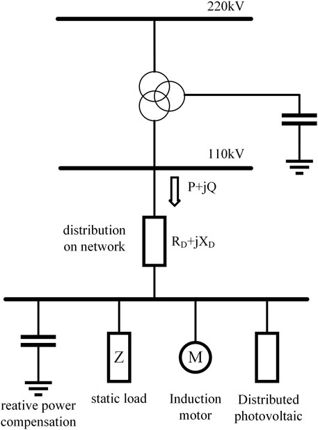
FIGURE 1. The composite load model with distributed photovoltaic power.

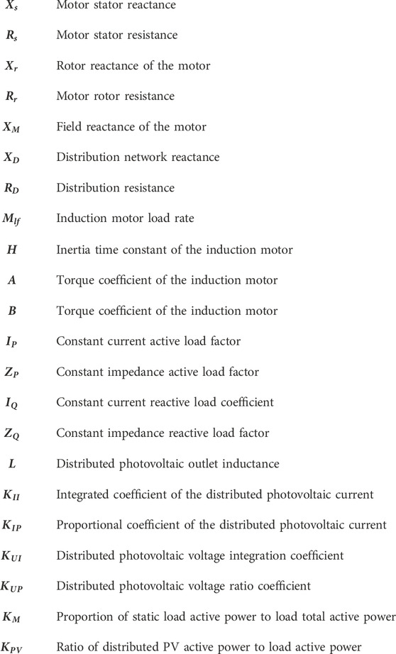
The distribution network model was composed of the distribution network impedance, the static load model was a constant impedance model, the dynamic load model was a third-order induction motor model, and the distributed photovoltaic power generation module was a double-loop controlled photovoltaic inverter model. Nomenclature presents the model parameters and a description of the composite load model with distributed photovoltaic power.

3.2 Main parameter set of the load model

In this study, multiple load model parameters were considered. When selecting the load parameters, the parameters that significantly impact the output response of the load were generally selected, while typical values were used for the remaining parameters. This concept is also used to analyze the effect of load parameters on dynamic security-region boundaries. The parameter changes that have a greater impact on the load output also have a greater influence on the transient stability of the system. Conversely, parameters having a smaller impact on the load output also have a smaller impact on the transient stability of the system. Based on the analysis of the TVSR, the transient voltage response of the load bus was selected as the reference basis to determine the effect of the load parameters on the output.

The trajectory sensitivity method was used to calculate the sensitivity of the load parameters and to determine the parameter set that significantly affects the load voltage response. The calculation formula for the trajectory sensitivity is as follows:

${\mathit{S}}_{\mathit{i}\mathit{j}}\left(\mathit{t}\right)=\frac{\mathit{\partial }{\mathit{y}}_{\mathit{i}}\left(\mathit{t}\right)/{\mathit{y}}_{\mathit{i}}\left(\mathit{t}\right)}{\mathit{\partial }{\mathit{\theta }}_{\mathit{j}}/{\mathit{\theta }}_{\mathit{j}}}=\underset{∆{\mathit{\theta }}_{\mathit{j}}\to \mathbf{0}}{\mathbf{lim}}\frac{\left[{\mathit{y}}_{\mathit{i}}\left({\mathit{\theta }}_{\mathit{j}\mathbf{0}}+∆{\mathit{\theta }}_{\mathit{j}},\mathit{t}\right)-{\mathit{y}}_{\mathit{i}}\left({\mathit{\theta }}_{\mathit{j}\mathbf{0}},\mathit{t}\right)\right]/{\mathit{y}}_{\mathit{i}}\left({\mathit{\theta }}_{\mathit{j}\mathbf{0}},\mathit{t}\right)}{∆{\mathit{\theta }}_{\mathit{j}}/{\mathit{\theta }}_{\mathit{j}\mathbf{0}}}.(4)$

Here, ${\mathit{\theta }}_{\mathit{j}}$ denotes the $\mathit{j}-\mathit{t}\mathit{h}$ parameter, ${\mathit{\theta }}_{\mathit{j}\mathbf{0}}$ and $∆{\mathit{\theta }}_{\mathit{j}}$ represent the initial value and variation in the parameter ${\mathit{\theta }}_{\mathit{j}}$, respectively, and ${\mathit{y}}_{\mathit{i}}$ denotes the trajectory of the $\mathit{i}-\mathit{t}\mathit{h}$ output variable, which represents the bus voltage response of the transient process load. In this paper, the variable $∆{\mathit{\theta }}_{\mathit{j}}/{\mathit{\theta }}_{\mathit{j}\mathbf{0}}$ of the parameter is set to be 10%. The load model described in this study was built into the simulation software application, and a transient fault was set up for the transient simulation. First, the initial value of the load model was set as a typical value, and each parameter in the load was then increased by 10%, corresponding to the initial value. The voltage-response data on the load bus within 3 s of the occurrence of a transient fault were selected as valid data for the calculation. Figure 2 presents the calculation results for the trajectory sensitivity for each load parameter.

FIGURE 2

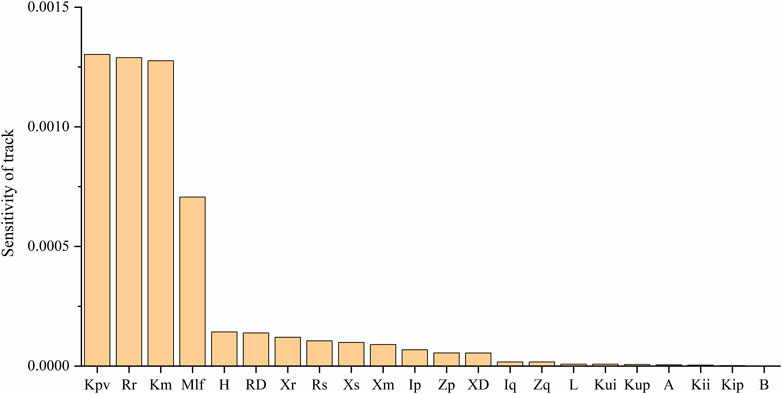
FIGURE 2. Calculation of trajectory sensitivity of load parameters.

The analysis in Figure 2 shows that the sensitivity of the four parameters, ${\mathit{K}}_{\mathit{M}}$, ${\mathit{K}}_{\mathit{P}\mathit{V}}$, ${\mathit{R}}_{\mathit{r}}$, and ${\mathit{M}}_{\mathit{l}\mathit{f}}$, is high, whereas the sensitivity of the other parameters was low. The low-sensitivity parameters do not significantly affect the system stability; therefore, they were not analyzed in this study. The load parameters set for this study were as follows:

$\mathit{p}=\left\{{\mathit{K}}_{\mathit{M}},{\mathit{K}}_{\mathit{P}\mathit{V}},{\mathit{R}}_{\mathit{r}},{\mathit{M}}_{\mathit{l}\mathit{f}}\right\},(5)$

where ${\mathit{K}}_{\mathit{M}}$ denotes the ratio of the active power of the dynamic load to the active power of the total load, ${\mathit{K}}_{\mathit{P}\mathit{V}}$ denotes the ratio of the active power of the distributed photovoltaic generation to the active power of the total load, ${\mathit{R}}_{\mathit{r}}$ denotes the stator resistance of the dynamic load, and ${\mathit{M}}_{\mathit{l}\mathit{f}}$ denotes the initial slip of the dynamic load.

4 The concept of the online TVSR boundary correction

4.1 Building the TVSR

The controllable variables of key nodes are often selected when constructing a power system security region. In selecting the critical nodes, different types of power system security regions are considered with different priorities. In this paper, we analyzed the construction of the TVSR; therefore, we focused more on the transient stability of the system, particularly the system voltage stability caused by load power fluctuation.

A composite load model with distributed photovoltaic power was built at BUS18 of the IEEE39 node system. Figure 3 presents a diagram of the system structure. Depending on the load used in this study, the active power of the load is considered one of the node injection quantities for constructing the TVSR. For practical engineering applications, based on the node voltage sensitivity under the change of load parameters, we determine the generator node with the greatest influence from the change of load parameters and use the active power of the generator node as another injection amount for constructing the TVSR.

FIGURE 3

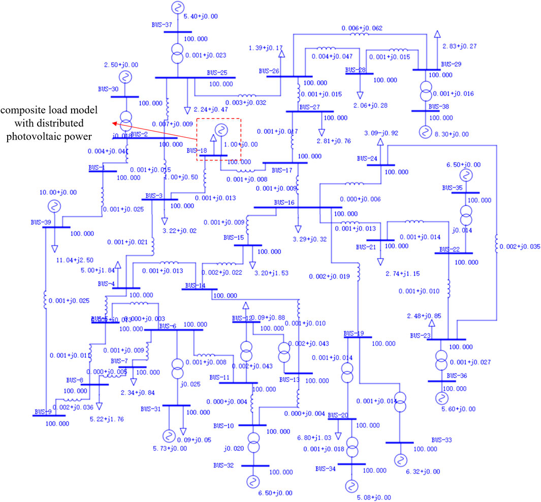
FIGURE 3. Wiring diagram of the IEEE39 node system.

The sensitivity of the transient voltage response of the generator node is calculated using the trajectory sensitivity method. Eq. 4 presents the calculation formula for trajectory sensitivity. The calculation process and method are approximately identical to those in the analysis of the sensitivity of the load parameters in Section 2.2. The trace sensitivity values of the four parameters in the load parameter set are defined as ${\mathit{S}}_{\mathit{K}\mathit{m}}$, ${\mathit{S}}_{\mathit{R}\mathit{r}}$, ${\mathit{S}}_{\mathit{M}\mathit{l}\mathit{f}}$, and ${\mathit{S}}_{\mathit{K}\mathit{p}\mathit{v}}$. The locus sensitivity of the transient voltage response of the system bus corresponding to the load active power is defined as ${\mathit{S}}_{\mathit{P}\mathit{L}\mathit{o}\mathit{a}\mathit{d}}$. The total track sensitivity, ${\mathit{S}}_{\mathit{s}\mathit{u}\mathit{m}}$, of the $\mathit{i}\mathit{t}\mathit{h}$ bus in the system is expressed as follows:

${\mathit{S}}_{\mathit{s}\mathit{u}\mathit{m},\mathit{i}}={\mathit{S}}_{\mathit{K}\mathit{m},\mathit{i}}+{\mathit{S}}_{\mathit{R}\mathit{r},\mathit{i}}+{\mathit{S}}_{\mathit{M}\mathit{l}\mathit{f},\mathit{i}}+{\mathit{S}}_{\mathit{K}\mathit{p}\mathit{v},\mathit{i}}+{\mathit{S}}_{\mathit{P}\mathit{L}\mathit{o}\mathit{a}\mathit{d},\mathit{i}}.(6)$

Figure 4 presents the calculation results for the load power and node voltage sensitivity of the four load parameters.

FIGURE 4

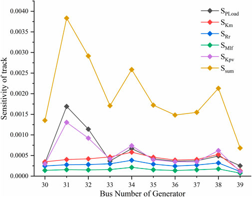
FIGURE 4. Transient voltage trace sensitivity of generator nodes in the IEEE39 node system.

According to the analysis in Figure 4, the generator nodes had the highest trajectory sensitivity, except for the equilibrium nodes BUS31, BUS32, and BUS34. Therefore, the two-dimensional (2D) and three-dimensional (3D) TVSR were constructed using the three-node controllable injection quantities of the active generator power of the BUS32 and BUS34 nodes and the active load power of the BUS18 nodes. For the construction of a 2D TVSR, a combination of the active power and load active power of any generator was selected. Conversely, the construction of a 3D TVSR involved selecting a combination of the active power and load active power of the two generators. The fluctuation range of the load power during the operation of the transmission network was approximately 40%. Therefore, the TVSR was constructed in the range of 80%–120% of the initial active power of the load. A point-by-point method was used to explore the TVSR boundary to determine the unknown TVSR boundary characteristics.

The three-phase short circuit was set at 50% of the line between buses BUS18 and BUS17 of the system load, with the short-circuit time set to 0.1 s. The voltage stability of the system bus was considered the criterion. In other words, when the transient process causes the voltage of the system bus to be lower than 0.7 p.u. for more than 1 s, the voltage instability of the system is determined. The critical instability points of the TVSR boundary were identified point-by-point using the fitting method.

4.2 Analysis of boundary characteristics

The changes in the TVSR boundary characteristics caused by the changes in the four parameters in the load parameter set $\mathit{p}$ were analyzed. According to the recommended IEEE parameters and the load model structure built in this study, the range of the load parameter changes is as follows: 1) $K_M$ is 0%–100%, 2) $K_{PV}$ is 0–1, 3) $R_r$ is 0.01 p.u. to 0.1 p.u., and 4) $M_{lf}$ is 0.1 p.u. to 0.8 p.u. Considering generators No. 32 and 34 (with the highest trajectory sensitivity) as examples, this study analyzed the characteristics of two 2D DSR boundaries comprising the active load power and active power of two generators, respectively, when the load parameters at BUS18 changed. Figure 5 shows the 2D TVSR boundaries under the changes in the four load parameters.

FIGURE 5

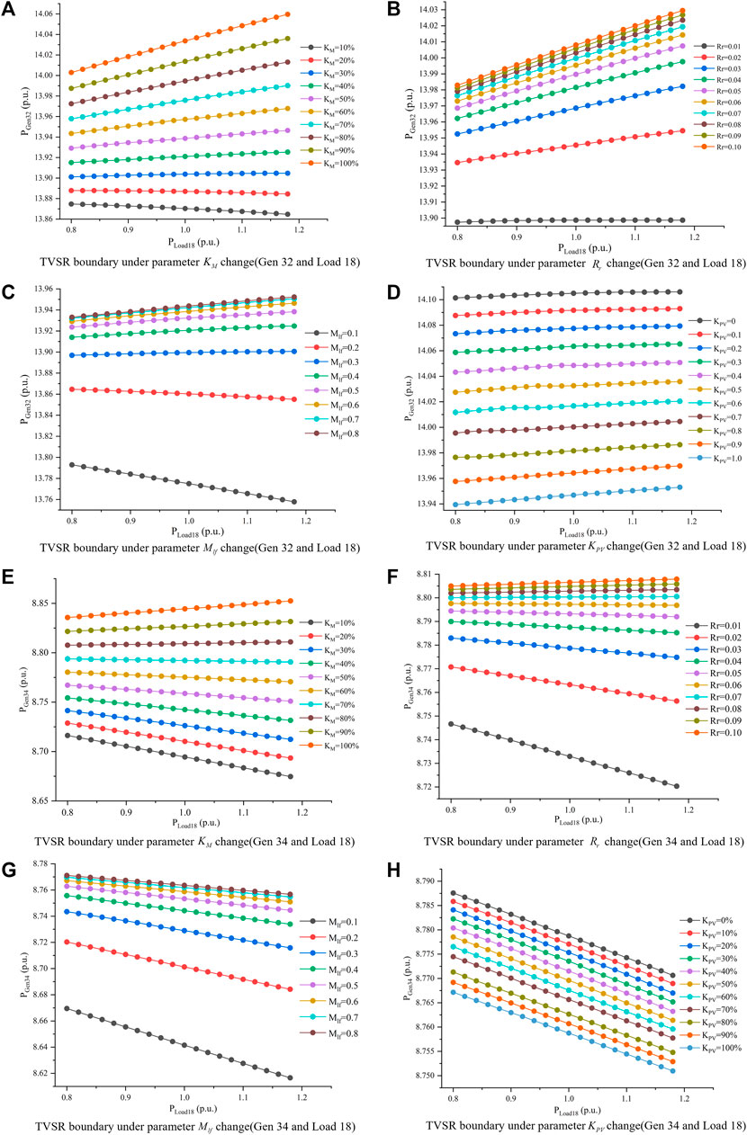
FIGURE 5. Two-dimensional TVSR boundary of IEEE39 node system influenced by load parameters.

When a single load parameter is represented by each subgraph in Figure 5, the other load parameters adopt typical values. Notably, the variation in the load parameters significantly affects the TVSR boundary in the figure, which was linearly fitted. The sum of squared errors (SSE), R², and the root mean squared error (RMSE) were calculated as 4.4366E-8, 0.9990, and 4.1959E-5, respectively. Through verification, it was determined that the 2D TVSR boundary analyzed in this study presented good linear characteristics within the scope of the engineering applications and that the linear fitting error was minimal.

The 3D TVSR boundary, comprising the generator at BUS32 and BUS34, and the load at BUS18 can be represented by multiple sets of 2D linear TVSR boundaries. Figure 6 shows the 3D TVSR boundary when typical load parameters are adopted.

FIGURE 6

FIGURE 6. IEEE39 node system 3D TVSR boundary.

4.3 Online correction of the TVSR boundary

Based on the analysis of the TVSR boundary characteristics in the previous section, it can be observed that the 2D TVSR boundary exhibited good linear characteristics. The TVSR boundary in a 2D plane can be represented by the set ${\mathit{l}}_{\mathit{n},\mathit{i},\mathit{j}}$, which is given as follows:

${\mathit{l}}_{\mathit{n},\mathit{i},\mathit{j}}=\left\{\left({\mathit{P}}_{\mathit{G}\mathit{e}\mathit{n},\mathit{i},\mathit{n}},{\mathit{P}}_{\mathit{L}\mathit{o}\mathit{a}\mathit{d},\mathit{j},\mathit{n}}\right)\left|{\mathit{P}}_{\mathit{G}\mathit{e}\mathit{n},\mathit{i},\mathit{n}}-{\mathit{k}}_{\mathbf{1},\mathit{n}}{\mathit{P}}_{\mathit{L}\mathit{o}\mathit{a}\mathit{d},\mathit{j},\mathit{n}}-{\mathit{k}}_{\mathbf{2},\mathit{n}}=\mathbf{0},{\mathit{P}}_{\mathit{L}\mathit{o}\mathit{a}\mathit{d},\mathit{j},\mathit{n}}\in \left[{\mathit{P}}_{\mathit{L}\mathit{o}\mathit{a}\mathit{d},\mathit{j},\mathit{min}},{\mathit{P}}_{\mathit{L}\mathit{o}\mathit{a}\mathit{d},\mathit{j},\mathit{max}}\right]\right.\right\},(7)$

where $\mathit{n}$ represents the $\mathit{n}-\mathit{t}\mathit{h}$ scenario under different load parameter combinations, $\mathit{i}$ represents the generator node number, $\mathit{j}$ represents the load node number, ${\mathit{P}}_{\mathit{G}\mathit{e}\mathit{n}}$ represents the active power of the generator under the critical instability state of TVSR, ${\mathit{P}}_{\mathit{L}\mathit{o}\mathit{a}\mathit{d}}$ represents the active power of the load under the critical instability state of TVSR, ${\mathit{k}}_{\mathbf{1}}$ and ${\mathit{k}}_{\mathbf{2}}$ represent the linear characteristics of the TVSR boundary, and ${\mathit{P}}_{\mathit{L}\mathit{o}\mathit{a}\mathit{d},\mathit{j},\mathit{min}}$ and ${\mathit{P}}_{\mathit{L}\mathit{o}\mathit{a}\mathit{d},\mathit{j},\mathit{max}}$ represent the maximum and minimum values of active power when the $\mathit{j}-\mathit{t}\mathit{h}$ load runs, respectively.

To determine the 2D TVSR boundary in scenario $\mathit{n}$ comprising any combination of load parameters, the values of coefficients ${\mathit{k}}_{\mathbf{1}}$ and ${\mathit{k}}_{\mathbf{2}}$ must be determined. Therefore, two equations must be constructed and solved. This requires the knowledge of two critical points on the TVSR boundary in each scenario. Eq. 7 requires two equations to be constructed by obtaining two pairs of values of ${\mathit{P}}_{\mathit{G}\mathit{e}\mathit{n}}$ and ${\mathit{P}}_{\mathit{L}\mathit{o}\mathit{a}\mathit{d}}$ in scenario $\mathit{n}$. However, there are infinite permutations and combinations of the four load parameter values. Therefore, two running points on the new TVSR boundary must be calculated each time a new load parameter combination scenario appears. Nonetheless, using the point-by-point method to identify the boundary points is very time-consuming and cannot adapt to the rapidly changing load parameters.

Therefore, this study uses a combination of load parameters as the input and the critical point of the TVSR as the output. A machine learning algorithm was then used to explore the correlation between different load parameter combinations and the critical instability point of the TVSR boundary. Thus, the online calculation of the TVSR boundary under different load parameter combinations can be realized. In this study, we use the CatBoost algorithm as a framework for machine learning.

During the calculation and analysis of the leading parameters of the load model, the extracted leading parameters were essentially identical when calculating the trajectory sensitivity of the leading parameters since the same models were used. When selecting key generator nodes for power systems with different structures, the key nodes of different systems vary due to the considerable differences in the system structure and parameters. Therefore, when TVSR boundary correction is performed, the key generator nodes must be rescreened based on the different systems and faults. Figure 7 shows the overall process of the rapid boundary correction of 2D TVSR.

FIGURE 7

FIGURE 7. Overall process of TVSR boundary online correction.

The 3D TVSR boundary surface is obtained by fitting the linear boundaries of multiple 2D TVSR. The 3D TVSR boundary can be represented by the set ${\mathit{\alpha }}_{\mathit{n},\mathit{i},{\mathit{i}}^{\prime },\mathit{j}}$, which is given as follows:

${\mathit{\alpha }}_{\mathit{n},\mathit{i},{\mathit{i}}^{\prime },\mathit{j}}=\left\{\left({\mathit{P}}_{\mathit{G}\mathit{e}\mathit{n},\mathit{i},\mathit{n}},{\mathit{P}}_{\mathit{G}\mathit{e}\mathit{n},{\mathit{i}}^{\prime },\mathit{n}},{\mathit{P}}_{\mathit{L}\mathit{o}\mathit{a}\mathit{d},\mathit{j},\mathit{n}}\right)\left|{\mathit{P}}_{\mathit{G}\mathit{e}\mathit{n},\mathit{i},\mathit{n}}-{\mathit{k}}_{\mathbf{1},\mathit{n}}{\mathit{P}}_{\mathit{L}\mathit{o}\mathit{a}\mathit{d},\mathit{j},\mathit{n}}-{\mathit{k}}_{\mathbf{2},\mathit{n}}=\mathbf{0},{\mathit{P}}_{\mathit{L}\mathit{o}\mathit{a}\mathit{d},\mathit{j},\mathit{n}}\in \left[{\mathit{P}}_{\mathit{L}\mathit{o}\mathit{a}\mathit{d},\mathit{j},\mathit{min}},{\mathit{P}}_{\mathit{L}\mathit{o}\mathit{a}\mathit{d},\mathit{j},\mathit{max}}\right]\right.\right\},(8)$

where ${\mathit{i}}^{\prime }$ represents the node number of the second generator that constitutes the 3D TVSR plane. The other parameters in the formula have the same meanings, as those in Eq. 7. Therefore, after establishing the CatBoost training models under different ${\mathit{P}}_{\mathit{G}\mathit{e}\mathit{n},{\mathit{i}}^{\prime },\mathit{n}}$, a 3D TVSR plane can be fitted by calculating multiple sets of TVSR boundaries. Similarly, a high-dimensional TVSR boundary comprising more node generator active powers and load active powers was calculated.

5 Introduction to the algorithm

CatBoost is a gradient-boosting decision tree (GBDT) framework based on a symmetric decision tree that has fewer parameters, supports class-type variables, and exhibits high accuracy. The structure of a symmetric oblivious tree presents fewer super-parameters and faster training speed. CatBoost solves the problem of gradient bias and prediction shift by using the sorting promotion method to reduce the occurrence of overfitting and improve the accuracy and generalization ability of the algorithm. CatBoost displays superiority in processing missing values and noisy data and exhibits a certain tolerance for outliers and noise when compared to XGBoost and LightBoost, the two other mainstream algorithms of GBDT. Furthermore, the risk of overfitting can be reduced via the random arrangement and sampling of the training samples.

5.1 CatBoost iteration process

During model training, each iteration generates a weak learner and minimizes the loss function of the current iteration. Assuming that the loss function is $\mathit{L}[\mathit{y},\mathit{f}\left(\mathit{x}\right)$, the objective function ${\mathit{h}}^{\mathit{t}}$ of each iteration can be defined as follows:

${\mathit{h}}^{\mathit{t}}=\underset{\mathit{h}\in \mathit{H}}{\mathbf{arg}\mathbf{min}}\mathit{E}\mathit{L}\left[\mathit{y},{\mathit{F}}^{\mathit{t}-\mathbf{1}}\left(\mathit{x}\right)+\mathit{h}\left(\mathit{x}\right)\right],(9)$

where ${\mathit{h}}^{\mathit{t}}$ denotes the tree selected from a series of $\mathit{H}$ functions, $\mathit{E}$ denotes the expected function, and ${\mathit{F}}^{\mathit{t}-\mathbf{1}}\left(\mathit{x}\right)$ denotes the strong learner obtained in the last iteration.

The negative gradient, $-{\mathit{g}}^{\mathit{t}}\left(\mathit{x},\mathit{y}\right)=-\mathit{\partial }\mathit{L}\left[\mathit{y},{\mathit{F}}^{\mathit{t}-\mathbf{1}}\left(\mathit{x}\right)\right]/\mathit{\partial }{\mathit{F}}^{\mathit{t}-\mathbf{1}}\left(\mathit{x}\right)$, of the loss function is the direction in which the error decreases the fastest. It is used to fit the loss approximation of each iteration, and the objective function ${\mathit{h}}^{\mathit{t}}$ can be expressed as follows:

${\mathit{h}}^{\mathit{t}}={\underset{\mathit{h}\in \mathit{H}}{\mathbf{arg}\mathbf{min}}\mathit{E}\left[-{\mathit{g}}^{\mathit{t}}\left(\mathit{x},\mathit{y}\right)-\mathit{h}\left(\mathit{x}\right)\right]}^{\mathbf{2}}.(10)$

Subsequently, the strong learner of this iteration is obtained as follows:

$\mathit{F}{\left(\mathit{x}\right)}^{\mathit{t}}=\mathit{F}{\left(\mathit{x}\right)}^{\mathit{t}-\mathbf{1}}+\mathit{\alpha }{\mathit{h}}^{\mathit{t}},(11)$

where $\mathit{\alpha }$ denotes the learning rate of the model.

5.2 Sort promotion

In the iteration process, the GBDT algorithm uses the same training samples to calculate the iteration gradient in each round. Eq. 10 can then be expressed as follows:

${\mathit{h}}^{\mathit{t}}=\underset{\mathit{h}\in \mathit{H}}{\mathbf{arg}\mathbf{min}}\frac{\mathbf{1}}{\mathit{n}}{\displaystyle {\sum }_{\mathit{k}-\mathbf{1}}^{\mathit{n}}}{\left[-{\mathit{g}}^{\mathit{t}}\left({\mathit{x}}_{\mathit{k}},{\mathit{y}}_{\mathit{k}}\right)-\mathit{h}\left({\mathit{x}}_{\mathit{k}}\right)\right]}^{\mathbf{2}},(12)$

where $\mathit{n}$ denotes the number of training samples and $\left.{\left\{\mathit{x}\right.}_{\mathit{k}},{\mathit{y}}_{\mathit{k}}\right\}$ denotes the $\mathit{k}$ training samples, where ${\mathit{y}}_{\mathit{k}}\in \left\{\mathbf{0,1}\right\}$.

This leads to a deviation between the gradient distribution ${{\mathit{g}}^{\mathit{t}}(\mathit{x}}_{\mathit{k}},{\mathit{y}}_{\mathit{k}})\left|{\mathit{x}}_{\mathit{k}}\right.$ obtained from the training sample and the real gradient distribution ${\mathit{g}}^{\mathit{t}}\left(\mathit{x},\mathit{y}\right)\left|\mathit{x}\right.$ o in the data space (Yu et al., 2006; Dorogush et al., 2018). The objective function determined using Eq. 12 deviates from the objective function in Eq. 9, which affects the accuracy and generalization ability of the model $\mathit{F}\left(\mathit{x}\right)$.

The CatBoost algorithm adopts the sorting and lifting method to perform the unbiased calculation of the gradient, which is based on the following principle. For each sample ${\mathit{x}}_{\mathit{i}}$, the training set excluding ${\mathit{x}}_{\mathit{i}}$ is used to train a model, ${\mathit{M}}_{\mathit{i}}$, separately, and ${\mathit{M}}_{\mathit{i}}$ is used to calculate the gradient on ${\mathit{x}}_{\mathit{i}}$. Dorogush et al. (2018) and Prokhorenkova et al. (2017) demonstrated the effectiveness of the sorting promotion method.

5.3 Algorithm hyperparameter settings

Owing to the ability of CatBoost to achieve high model quality without tuning parameters, most CatBoost hyperparameters were set to default values in this study. The main self-set parameters and their values were set as follows: iterations to 8,000, learning rate to 0.1, and depth to 3. The default values of the other parameters were retained.

6 Case study and result

6.1 Calculation and analysis of the IEEE39 node system

In this study, an IEEE39 node was used as an example to verify the proposed method. The composite load model with distributed photovoltaic power is built at BUS18. Based on the analysis in Section 3, the active power of the load being analyzed and that of the generator at BUS32 were selected as the injection quantities to construct the 2D TVSR. In total, 5,000 groups of parameter combinations were generated uniformly and randomly within the range of the load parameters listed in Table 1 to construct 5,000 different types of system operation scenarios. When the active power consumed by BUS18 load was 0.9 and 1.1 p.u., the fitting method was used to search the critical active power running points of BUS32 point-by-point, and 5,000 training samples were constructed.

TABLE 1

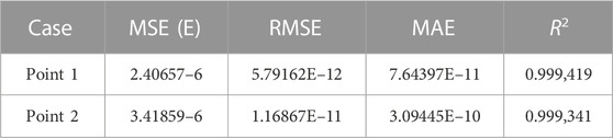
TABLE 1. IEEE39 node example of CatBoost learning framework verification indicators.

Two CatBoost learning frameworks were constructed and trained for two TVSR boundary points in each load–parameter combination scenario. The parameter combination in the constructed training sample was used as the input for the CatBoost learning framework, and the TVSR boundary point corresponding to the parameter combination was used as the output. To train and verify the model, we selected 80% of the data for the training set and 20% for the verification set.

The model training hyperparameters were automatically selected using CatBoost based on the number of training sets and their feature structure. The mean value of 100 iterations for the CatBoost-independent training and calculation results was used to calculate the regression validation indicators, such as the MSE, RMSE, the mean absolute error (MAE), and R² of the validation sets, as shown in Table 1.

We selected an untrained load parameter combination scenario and fed the load parameter combination into the trained CatBoost framework as an input. The TVSR boundary expression is calculated based on the outputs of the two TVSR boundary points. The calculated TVSR boundary is compared with the actual TVSR boundary, as shown in Figure 8A.

FIGURE 8

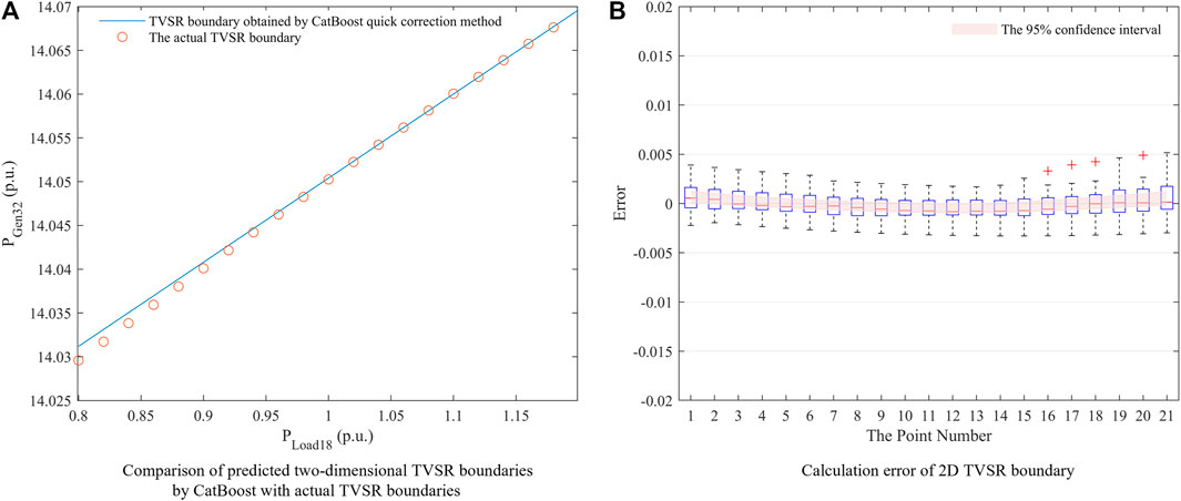
FIGURE 8. Schematic diagram of 2D TVSR boundary fitting for IEEE39 node system and calculation error.

An error analysis of the 2D TVSR boundary calculated by CatBoost was then performed as follows. The TVSR boundary point was ascertained using the verification set based on Eq. 7. A total of 21 boundary points were uniformly identified on the P load axis of the 2D TVSR space, with the error between the 21 and the real boundary points of the system calculated. The error distribution between the TVSR boundary obtained using the proposed method and the actual TVSR boundary was also determined. Figure 8B shows the error bars and 95% confidence intervals of the errors.

According to the analysis in Table 1, the CatBoost calculation method presents better prediction performance for the TVSR boundary points in scenarios with different load parameters, and a small number of training sets can be used to obtain higher prediction accuracy. Based on the analysis shown in Figure 8, the fast TVSR boundary correction method based on load parameter changes in the IEEE39 standard example system presents a high boundary fitting accuracy, and the calculated results are relatively reliable.

6.2 Calculation and analysis of the IEEE118 node system

The proposed method was verified in the case of IEEE118 nodes. Load 59, with high power on BUS59, was selected as the research object, with its model changed to a composite load model with distributed photovoltaic power. The active and reactive power of the load remained unchanged, and the added distributed PV active power was 50 MW. Figure 9 shows the wiring diagram of the modified example. The load model parameters were set to typical values, and a three-phase short circuit was set at 50% of the transmission line between BUS59 and BUS61 with a short circuit time of 0.1 s. The trajectory sensitivity of the bus voltage of each generator was calculated corresponding to the load parameters and load active power under transient fault conditions.

FIGURE 9

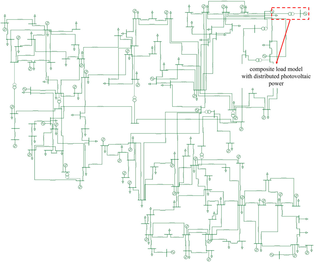
FIGURE 9. Wiring diagram of the IEEE118 node system.

The transient voltage locus sensitivities of the BUS116 and BUS65 nodes were relatively high, as shown in Figure 10. Therefore, the active power of the Gen116 and Gen65 generators and the active power of Load 59 were selected as the node injection quantities to construct 2D and 3D TVSR. The effects of different load parameters on the TVSR boundary in two 2D spaces constructed using the load active power and the active power of the two generators were calculated, as shown in Figure 11. Figure 12 shows the TVSR boundary in 3D space with typical parameter values for the load.

FIGURE 10

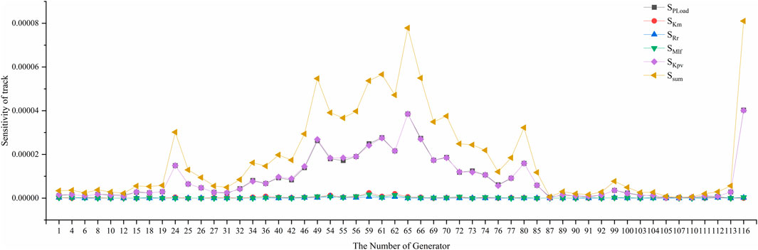
FIGURE 10. Transient voltage trace sensitivity of generator nodes in the IEEE118 node system.

FIGURE 11

FIGURE 11. Two-dimensional TVSR boundary of IEEE118 node system influenced by load parameters.

FIGURE 12

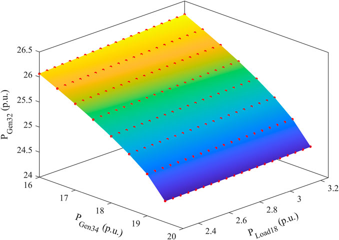
FIGURE 12. IEEE118 node system 3D TVSR boundary.

The TVSR boundary shown in the figure was linearly fitted. The SSE, R², and RMSE values were calculated as 5.2956E-6, 0.9997, and 5.3940E-4, respectively.

The range of the load parameter changes is as follows: 1) $K_M$ is 0%–100%, 2) $K_{PV}$ is 0–0.18, 3) $R_r$ is 0.01–0.1 p.u., and 4) $M_{lf}$ is 0.1–0.8 p.u. A total of 5,000 groups of parameter combinations were generated uniformly and randomly within the range of the load parameters to construct 5,000 system operation scenarios. When the unit value of active power consumed by the BUS59 load is 2.4 and 3.1 p.u. respectively, the fitting method is used to search for the critical active power running point of BUS116 point-by-point, and 5,000 training samples are constructed.

Similar to the calculation of the IEEE39 nodes, two CatBoost learning frameworks were constructed and trained, respectively. Furthermore, 80% of the data were selected as the training set and 20% as the verification set. Table 2 lists the averaged verification results of 100 independent CatBoost training sessions.

TABLE 2

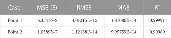
TABLE 2. IEEE118 node example of CatBoost learning framework verification indicators.

Any group of the calculated TVSR boundaries was selected and compared with the real TVSR boundaries, as shown in Figure 13A.

FIGURE 13

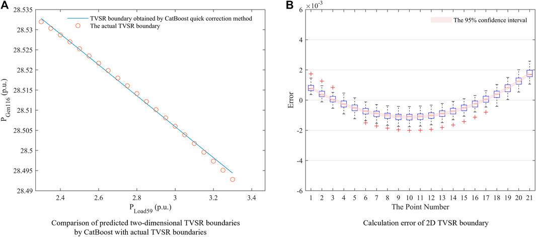
FIGURE 13. Schematic diagram of 2D TVSR boundary fitting for IEEE118 node system and calculation error.

The error distribution between the TVSR boundary obtained using the proposed method and the actual TVSR boundary was calculated. Figure 13B shows the error bars and 95% confidence intervals of the errors.

The data in Table 2 show CatBoost exhibits high calculation accuracy and produces reliable results in the calculation examples of the IEEE118 nodes. The analysis presented in Figure 13 highlights that the TVSR boundary calculated using the proposed method exhibits a good fitting effect with high fitting accuracy. The load parameter change of the IEEE39 node system exerts a lesser effect on the TVSR boundary than that of the IEEE118 node system, and the range of the boundary change is smaller. This results in the variance in the error distribution of the IEEE118 node system from that of the IEEE39 node system. Therefore, the TVSR boundary fitting error of the IEEE118 nodes was smaller than that of the IEEE39 nodes, and the error distribution was more compact.

The proposed TVSR online correction method trains the CatBoost network offline, inputs the CatBoost network online based on the change in the load parameters, and outputs the TVSR boundary online without delay. Therefore, it only requires time to train the model and does not perform complex calculations in online applications. The results are directly output by the model, which satisfies the demand for fast online applications.

Based on the calculation and verification of the IEEE39 and IEEE118 node systems, the proposed method can complete the training of the CatBoost network in the offline state to realize fast correction of the TVSR boundary of the power system online and satisfy the demands of the rapidly changing load. This capability addresses the requirements of dynamically changing loads, which is crucial for network regulation and security of power systems.

7 Conclusion

In this study, we used a composite load model with distributed photovoltaic power as the research object to comprehensively analyze the influence of the load model parameters on the TVSR of a smart grid. The trajectory sensitivity method was employed to determine the main voltage stability parameters of the load model that significantly affect the transient response of the node voltage. Furthermore, the trajectory sensitivity method was employed to determine the main generator node sensitive to the load parameters and load power changes. The main generator node and node active power of the load are used as the injection amounts to construct the TVSR in this project. Considering the 2D and 3D TVSR space as an example, it was observed that the boundary characteristics of the TVSR present a good linear effect within the range of the normal variation in the load active power, which helps in deriving the TVSR boundary expression. We proposed a fast TVSR boundary correction method based on the CatBoost learning framework. The various combination scenarios of the dominant parameter set of voltage stability under different loads were constructed offline, and the parameter combinations were considered inputs, while the TVSR boundary points were considered outputs to train the CatBoost model offline. Based on the trained CatBoost model and the TVSR expression, the TVSR boundary can be modified online, corresponding to the real-time changes in the load parameters. The proposed TVSR boundary correction method was verified based on the IEEE39 and IEEE118 node systems. The calculated results exhibited a high degree of fitness to the TVSR boundary along with good engineering practicability. The proposed TVSR boundary online correction method can correct the TVSR boundary online with high precision based on real-time changes in the load model parameters. This can provide a more accurate TVSR boundary, aiding the power system operation scheduler in controlling the system more accurately.

Data availability statement

The original contributions presented in the study are included in the article/Supplementary Material; further inquiries can be directed to the corresponding author.

Author contributions

The paper was completed with the joint efforts of five authors; each of them has made their own contributions to the model, algorithm, data, and other aspects. ZZ: conceptualization and methodology. ZY: supervision. ZY: writing—original draft. QC: software. MJ: translation. MD: resources. All authors contributed to the article and approved the submitted version.

Funding

This work was supported by the National Natural Science Foundation of China (52177106).

Conflict of interest

Author DM was employed by State Grid Jibei Electric Power Company Limited. Author QC was employed by State Grid Economic and Technological Research Institute Co., Ltd.

The remaining authors declare that the research was conducted in the absence of any commercial or financial relationships that could be construed as a potential conflict of interest.

Publisher’s note

All claims expressed in this article are solely those of the authors and do not necessarily represent those of their affiliated organizations, or those of the publisher, the editors, and the reviewers. Any product that may be evaluated in this article, or claim that may be made by its manufacturer, is not guaranteed or endorsed by the publisher.

References

Arif, A., Wang, Z., Wang, J., Mather, B., Bashualdo, H., and Zhao, D. (2018). Load modeling—a review. IEEE Trans. Smart Grid 9 (6), 5986–5999. doi:10.1109/TSG.2017.2700436

CrossRef Full Text | Google Scholar

Avila, N. F., Callegaro, L., and Fletcher, J. (2020). “Measurement-based parameter estimation for the WECC composite load model with distributed energy Resources,” in Proccedings of the 2020 IEEE Power & Energy Society General Meeting (PESGM), Montreal, QC, Canada, August 2020, 1–5. doi:10.1109/PESGM41954.2020.9281843

CrossRef Full Text | Google Scholar

Dorogush, A. V., Ershov, V., and Gulin, A. (2018). CatBoost: gradient boosting with categorical features support. Available at: https://arxiv.org/abs/1810.11363.

Google Scholar

Gaikwad, A., Markham, P., and Pourbeik, P. (2016). “Implementation of the WECC Composite Load Model for utilities using the component-based modeling approach,” in Proccedings of the 2016 IEEE/PES Transmission and Distribution Conference and Exposition (T&D), Dallas, TX, USA, May 2016, 1–5. doi:10.1109/TDC.2016.7520081

CrossRef Full Text | Google Scholar

Han, D., Ma, J., He, R. -m., and Dong, Z. -y. (2009). A real application of measurement-based load modeling in large-scale power grids and its validation. IEEE Trans. Power Syst. 24 (4), 1756–1764. doi:10.1109/TPWRS.2009.2030298

CrossRef Full Text | Google Scholar

Hu, F., Sun, K., Del Rosso, A., Farantatos, E., and Bhatt, N. B. (2016). “Measurement-based real-time voltage stability monitoring for load areas,” in Proccedings of the 2016 IEEE Power and Energy Society General Meeting (PESGM), Boston, MA, USA, July 2016, 1. doi:10.1109/PESGM.2016.7741116

CrossRef Full Text | Google Scholar

IEEE Standared Association (2020). “IEEE guide for load modeling and simulations for power systems,” in Proccedings of the IEEE Std 2781-2022, September 2022, 1–88. doi:10.1109/IEEESTD.2022.9905546

CrossRef Full Text | Google Scholar

Li, H., Fan, Y., and Wu, T. (2006). “Impact of load characteristics and low-voltage load shedding schedule on dynamic voltage stability,” in Proccedings of the 2006 Canadian Conference on Electrical and Computer Engineering, Ottawa, ON, Canada, May 2006, 2249–2252. doi:10.1109/CCECE.2006.277553

CrossRef Full Text | Google Scholar

Maihemuti, S., Wang, W., Wang, H., Wu, J., and Zhang, X. (2021). Dynamic security and stability region under different renewable energy permeability in IENGS system, in IEEE Access. 9 19800–19817. doi:10.1109/ACCESS.2021.3049236

CrossRef Full Text | Google Scholar

Mather, B. A. (2012). “Quasi-static time-series test feeder for PV integration analysis on distribution systems,” in Proccedings of the 2012 IEEE Power and Energy Society General Meeting, San Diego, CA, USA, July 2012, 1–8. doi:10.1109/PESGM.2012.6345414

CrossRef Full Text | Google Scholar

Meng, Y., Yuquan, L., Wen, X., Xin, L., Ying, C., and Yuquan, L. (2014). “Voltage stability research of receiving-end network based on real-time classification load model,” in Proccedings of the 2014 IEEE International Conference on Mechatronics and Automation, Tianjin, China, August 2014, 1866–1870. doi:10.1109/ICMA.2014.6885986

CrossRef Full Text | Google Scholar

Monteiro Pereira, R. M., Pereira, A. J. C., Machado Ferreira, C. M., and Maciel Barbosa, F. P. (2008). “Dynamic voltage stability assessment of an electric power network using composite load models,” in Proccedings of the 2008 43rd International Universities Power Engineering Conference, Padua, Italy, September 2008, 1–5. doi:10.1109/UPEC.2008.4651522

CrossRef Full Text | Google Scholar

Prokhorenkova, L., Gusev, G., Vorobev, A., et al. (2017). CatBoost: Unbiased boosting with categorical features.

Google Scholar

Rodríguez-García, L., Pérez-Londoño, S., and Mora-Florez, J. J. (2020). “Methodology for measurement-based load modeling considering integration of dynamic load models,” in Proccedings of the 2020 IEEE International Autumn Meeting on Power, Electronics and Computing (ROPEC), Ixtapa, Mexico, November 2020, 1–6. doi:10.1109/ROPEC50909.2020.9258723

CrossRef Full Text | Google Scholar

Soliman, S. A., Abbasy, N. H., and El-Hawary, M. E. (1997). Frequency domain modelling and identification of nonlinear loads using a least error squares algorithm. Electr. Power Syst. Res. 40 (1), 1–6. doi:10.1016/S0378-7796(96)01123-6

CrossRef Full Text | Google Scholar

Song, Y., and Blaabjerg, F. (2017). Overview of DFIG-based wind power system resonances under weak networks. IEEE Trans. Power Electron. 32 (6), 4370–4394. doi:10.1109/TPEL.2016.2601643

CrossRef Full Text | Google Scholar

Taylor, C. W. (1994). Power system voltage stability (the EPRI power system engineering series). New York, NY, USA: McGraw-Hill.

Google Scholar

Visconti, I. F., Lima, D. A., Costa, J. M. C. d. S., and Sobrinho, N. R. d. B. C. (2014). Measurement-based load modeling using transfer functions for dynamic simulations. IEEE Trans. Power Syst. 29 (1), 111–120. doi:10.1109/TPWRS.2013.2279759

CrossRef Full Text | Google Scholar

Wang, Y., Lu, C., Wu, P., Zhang, X., Su, Y., Xiong, C., et al. (2022). Online realization of an ambient signal-based load modeling algorithm and its application in field measurement data. IEEE Trans. Industrial Electron. 69 (7), 7451–7460. doi:10.1109/TIE.2021.3102428

CrossRef Full Text | Google Scholar

Xiran, W., Huaidong, L., Yanyang, F., and Wei, C. (2013). “Improved emergency control strategy with optimal control time based on dynamic security region,” in Proccedings of the 2013 IEEE International Conference of IEEE Region 10 (TENCON 2013), Xi'an, China, October 2013, 1–4. doi:10.1109/TENCON.2013.6718824

CrossRef Full Text | Google Scholar

Yixin, Yu., Yanli, Liu., Chao, Qin., and Tiankai, Yang. (2020). Theory and method of power system integrated security region irrelevant to operation states: an introduction. Engineering 6 (7), 754–777. doi:10.1016/j.eng.2019.11.016

CrossRef Full Text | Google Scholar

Yu, Yixin, Dong, Cun, Lee, StephenT., and Zhang, Pei (2006). Practical dynamic security region in complex power injection space. Tianjin: Journal of Tianjin University, 129–134.

Google Scholar

Yuan, Zeng, and Yu, Yixin (2002). A practical direct method for determining dynamic security regions of electrical power systems. Proc. Int. Conf. Power Syst. Technol. 2, 1270–1274. doi:10.1109/ICPST.2002.1047606

CrossRef Full Text | Google Scholar

Zeng, Y., Zhang, P., Wang, M., Jia, H., Yu, Y., and Lee, S. T. (2006). “Development of a new tool for dynamic security assessment using dynamic security region,” in Proccedings of the 2006 International Conference on Power System Technology, Chongqing, China, October 2006, 1–5. doi:10.1109/ICPST.2006.321756

CrossRef Full Text | Google Scholar

Zhang, P., Hu, W., Liu, X., Xu, X., and Shao, G. (2017). “Study on practical dynamic security region of power system based on big data,” in Proccedings of the 2017 12th IEEE Conference on Industrial Electronics and Applications (ICIEA), Siem Reap, Cambodia, June 2017, 1996–1999. doi:10.1109/ICIEA.2017.8283165

CrossRef Full Text | Google Scholar

Zhou, B., Zeng, Y., Zhen, Q., Wang, A., Xie, Y., and Sun, F. (2018). “Research on the transient stability influenced by wind farm access nodes based on dynamic security region,” in Proccedings of the 2018 China International Conference on Electricity Distribution (CICED), Tianjin, China, September 2018, 2044–2046. doi:10.1109/CICED.2018.8592528

CrossRef Full Text | Google Scholar

Zhu, L., Li, X., Ouyang, H., Wang, Y., Liu, W., and Shao, K. (2012). “Research on component-based approach load modeling based on energy management system and load control system,” in Proccedings of the IEEE PES Innovative Smart Grid Technologies, Tianjin, China, May 2012, 1–6. doi:10.1109/ISGT-Asia.2012.6303137

CrossRef Full Text | Google Scholar

Nomenclature