Low-carbon economic operation of integrated energy systems in consideration of demand-side management and carbon trading

Under the background of carbon emission abatement worldwide, carbon trading is becoming an important carbon financing policy to promote emission mitigation. Aiming at the emerging coupling among various energy sectors, this paper proposes a bi-level scheduling model to investigate the low-carbon operation of the electricity and natural gas integrated energy systems (IES). Firstly, an optimal energy flow model considering carbon trading is formulated at the upper level, in which carbon emission flow model is employed to track the carbon flows accompanying energy flows and identify the emission responsibility from the consumption-based perspective, and the locational marginal price is determined at the same time. Then at the lower level, a developed demand-side management strategy is introduced, which can manage demands in response to both the dynamic energy prices and the nodal carbon intensities, enabling the user side to participate in the joint energy and carbon trading. The bi-level model is solved iteratively and reaches an equilibrium. Finally, case studies based on the IEEE 39-bus system and the Belgium 20-node system illustrate the effectiveness of the proposed method in reducing carbon emissions and improving consumer surplus.

1 Introduction

With the increasingly severe energy crisis and environmental problems, energy conservation and emission reduction have become the consensus of all countries for sustainable development. According to the statistics provided by the International Energy Agency (IEA), electricity and heat industry accounts for more than 40% of the global CO₂ emissions in 2021 (IEA, 2022). Therefore, developing low-carbon electricity is of great significance to the control of carbon emissions.

The emerging integrated energy system (IES), as a carrier of multi-energy coupling, has been recognized as an efficient method to promote the consumption of renewable energy and reduce carbon emissions. A lot of efforts have been made on the coordinated optimization and market operation of the electricity and natural gas IES at present. In literature (Jiang et al., 2022), a bi-level strategic bidding model was proposed to study the market behaviors of the gas-fired units in interdependent electricity and natural gas markets. In literature (Chen et al., 2020), the operational equilibria of electric and natural gas systemswas obtained under different levels of temporal and spatial granularity. A mixed-integer linear programming (MILP) approach was addressed to solve the security-constrained joint expansion planning problems of natural gas and electricity transmission systems in literature (Zhang et al., 2018). Besides the transmission level, the energy hub (EH), which integrates multiple energy sources at the distribution level, plays an important role in energy production, transmission, conversion, and storage (Geidl and Andersson, 2007). The modeling (Wang et al., 2019), planning (Huang et al., 2019), and operation (Paudyal et al., 2015) of IES with EHs have also attracted extensive attention. However, the natural gas flow equation is nonlinear and nonconvex, which will bring great challenges to solve the IES operation problem. In literature (Zhang et al., 2018), piecewise linearization method was applied to convert the Weymouth equation into the MILP form, but the solution accuracy and efficiency were affected by the number of 0–1 variables. A second-order cone (SOC) relaxation method was proposed in literature (Borraz-Sánchez et al., 2016) for model convexification, while the relaxation would cause an optimality gap due to the expansion of the feasible region. How to solve the natural gas flow equation accurately and efficiently still needs to be studied in IES research.

Meanwhile, when considering the low-carbon operation of IES, low-carbon factors can be embedded into the problems with emission constraints (Olsen et al., 2019; Gu et al., 2020) or objective functions including environmental costs (Li et al., 2018). Moreover, the rise of carbon emission trading provides a market solution for carbon abatement and regulation, in which the cap-and-trade scheme has been proven as one of the most effective mechanisms in real-world implementations such as Europe (EMBER, 2021) and China (Fang et al., 2019). In the process of carbon cap-and-trade scheme, the government issues a set amount of permits to companies that comprise a cap on allowed CO₂ emissions, and companies that surpass the cap are taxed, while companies that cut their emissions may sell or trade the unused credits. In this context, the coordination of carbon trading and energy trading has become a common concern. Existing research has been conducted on how to develop a joint energy and carbon market scheme. An IES co-trading market including electricity, natural gas, and carbon trading was proposed in literature (Sun et al., 2022), where an improved Multi-agent Deep Deterministic Policy Gradient algorithm was applied to achieve fair trade and entity privacy protection. Literature (Liu, 2022) analyzed the characteristics of the carbon-electricity integrated market and constructed a carbon-electricity integrated optimal bidding model for the virtual power plant (VPP) with the consideration of multiple uncertainties. To promote local decarbonization, a peer-to-peer (P2P) joint electricity and carbon trading model to co-optimize the energy and carbon permit transactions considering the trading preferences in the distribution network was proposed in literature (Lu et al., 2023), in which a carbon-aware distribution locational marginal pricing was formulated to guide the P2P transactions among prosumers.

However, the works above normally focus on the “observed” emission and attribute the emission responsibility to the generation side. But it is a fact that end-users create the need for the combustion of fossil fuels and are the underlying driving force of emissions, the intuitive generation-based settlement cannot clarify the emission responsibility of the demand side, which may result in uneven incentives (Wang et al., 2020). Therefore, it is important to track the carbon emission path and identify emission amount from the perspective of energy users. A demand-side management (DSM) approach aiming at carbon footprint control was proposed in literature (Pourakbari-Kasmaei et al., 2020), which was proven fairer and superior compared to existing policies. The concept of carbon emission flow (CEF) was introduced in literature (Kang et al., 2015), where CEF was regarded as a virtual attachment to the power flow and accumulated at the demand side. On this basis, the CEF model was extended to the multiple energy systems (MESs) in literature (Cheng et al., 2019). The low-carbon operation of MESs by coordinating the transmission-level and distribution-level via the energy-carbon integrated prices was studied in literature (Cheng et al., 2020), in which the carbon emissions of different energy systems are uniformly priced using the CEF model. Although the CEF model provides a more accurate method for carbon accounting and a fairer way for emission responsibility clarification, the literatures mentioned above have not involved user-side participation in the joint energy and carbon trading process.

Accordingly, this paper proposes a bi-level economic operation model for the electricity and natural gas IES with the consideration of DSM and carbon trading. The proposed method relies on CEF model to obtain the overall carbon flow distribution, and guides demand response through the nodal carbon intensities (NCIs) and the locational marginal prices (LMPs), realizing the IES low-carbon economic dispatch with the participation of user side. The main contributions are summarized as follows.

1) The carbon-constrained locational electricity marginal price (LMEP) and locational marginal gas price (LMGP) are formulated to describe the impacts of carbon trading scheme to the demand side, where the sequential cone programming (SCP) method is applied to guarantee the strictness of the relaxation of natural gas flow equation.

2) A developed demand response model is introduced. Our model can manage energy users to adjust their demands by means of transfer or substitution in response to both the carbon emission intensities and the locational marginal prices.

3) A bi-level scheduling model is proposed to investigate the low-carbon economic operation of the IES. An optimal energy flow model aiming at minimizing the negative social welfare considering carbon trading is formulated at the upper level, and demands on the user side are managed to maximize the consumer surplus at the lower level. The two levels interact iteratively to reach an equilibrium.

The rest of this paper is organized as follows. Section 2 provides the formulations of the proposed model. The linearization method and iterative procedure are presented in Section 3. Section 4 provides case study results based on an actual IES. Finally, conclusions are drawn in Section 5.

2 Model formulations

2.1 Problem statement

Before building the mathematical model, we need to make the following assumptions:

1) Since the carbon emissions in the electricity network are mainly related to active power and rarely affected by reactive power, both power flow and carbon flow analyses of the electricity network in this paper use the DC power flow model, and carbon and network losses are ignored.

2) A simplified steady-state gas flow model without considering line-pack is adopted in this paper. The power system and natural gas system are coupled via gas-turbine units at the transmission level.

3) The electricity and gas supply and consumption are paid at LMEPs and LMGPs, which are determined by the independent system operator (ISO) and natural gas market operator (GMO) in the market clearing process, respectively.

4) Carbon trading exists not only on the generation side but also on the demand side. Energy users calculate their carbon emissions via the CEF model, and the carbon emission allowances for users are pre-determined.

On this basis, the proposed framework can be modeled as a hierarchical problem which contains two levels, as shown in Figure 1. The upper level is formulated as an optimal power flow problem to minimize the negative social welfare, including the power generation cost and the carbon trading cost at the generation side. Meanwhile, the carbon emission intensities of each bus in the IES and LMPs can be obtained at the upper level and transmitted to the lower level. At the lower level, energy users make a response to the indicators passed from the upper level to maximize their consumer surplus. In this process, energy users would be motivated to cut demands with high carbon emission intensities to get benefits in the carbon trading market at the demand side. Afterward, the updated electricity and gas demands are sent back to the upper level to reschedule the power output. This bi-level interaction procedure iterates until equilibrium is reached.

FIGURE 1

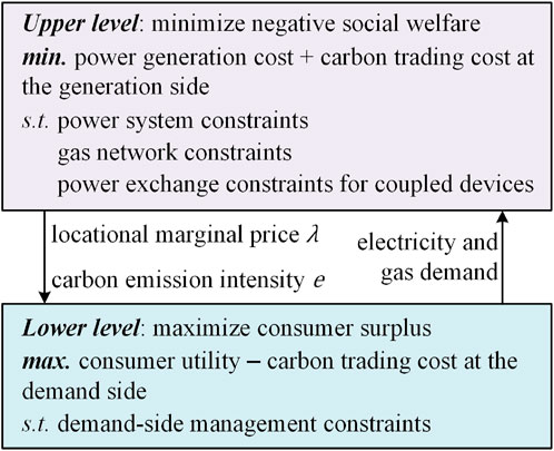
FIGURE 1. The framework of the proposed bi-level model.

2.2 Carbon emission model

Although CO₂ is directly emitted by generators, consumers are the main driving force of emissions due to energy use. Clarification of the emission responsibility is essential to mitigate carbon emissions. The CEF model can be used to trace the carbon emissions from the generation side to the demand side. In the CEF model, carbon emission intensity is one of the key indicators, which denotes the accompanying carbon emissions per unit of energy flow. In this paper, nodal carbon emission intensity (NCI) and branch carbon emission intensity (BCI) are mainly considered.

In the electricity network, for a given node $n$, its NCI can be represented as,

$\begin{array}{c}{e}_{n,t}^{EN}=\frac{{\sum }_{k:\left(k,n\right)\in {\mathrm{\Omega }}_n^{EN+}}\left|f_{kn,t}\right|\cdot {\rho }_{kn,t}^{line}+{\sum }_{i\in {\mathrm{\Omega }}_n^{TU}\cup {\mathrm{\Omega }}_n^{GT}}{P}_{Gi,t}\cdot e_{Gi}}{{\sum }_{k:\left(k,n\right)\in {\mathrm{\Omega }}_n^{EN+}}\left|f_{kn,t}\right|+{\sum }_{i\in {\mathrm{\Omega }}_n^{TU}\cup {\mathrm{\Omega }}_n^{GT}}{P}_{Gi,t}}\end{array}(1)$

where ${\mathrm{\Omega }}_n^{EN+}$, ${\mathrm{\Omega }}_n^{TU}$, and ${\mathrm{\Omega }}_n^{GT}$ denote the set of transmission lines that inject power into node $n$, the set of coal-fired thermal units connected to node $n$, and the set of gas-turbine units connected to node $n$, respectively. $f_{kn,t}$ and ${\rho }_{kn,t}^{line}$ are the power flow and the BCI of transmission line $kn$, respectively. $P_{Gi,t}$ and $e_{Gi}$ are the injected power and the carbon emission intensity of generator $i$, respectively.

And the BCI of the transmission line $kn$ can be expressed as,

$\begin{array}{c}{\rho }_{kn,t}^{line}=\left\{\begin{array}{c}{e}_{k,t}^{EN},if{f}_{kn,t}\ge 0\\ e_{n,t}^{EN},if{f}_{kn,t}<0\end{array}\right.\end{array}(2)$

Based on the results of NCI and BCI, the emission accounting can be implemented in a fairer way. Specifically, for the supply side, the carbon emission amount $E_{Gi,t}$ of generator $i$ can be calculated as follows,

$\begin{array}{c}{E}_{Gi,t}=P_{Gi,t}\cdot e_{Gi}\cdot \Delta t,\forall i\in {\mathrm{\Omega }}_n^{TU}\cup {\mathrm{\Omega }}_n^{GT},t\end{array}(3)$

where $\Delta t$ is the time interval. Note here we treat $e_{Gi}$ as a time-independent known parameter since for a single generator, its carbon emission intensity, which is also known as the generation carbon intensity (GCI), can be determined by the carbon emission factor of fuel and its fuel consumption rate, and we consider it to be an inherent generator parameter similar to the generation cost coefficient (i.e. a, b, c).

For the demand side, the “virtual” carbon emission amount $E_{Dn,t}$ due to the nodal power consumption $P_{Dn,t}$ can be obtained in the same way,

$\begin{array}{c}{E}_{Dn,t}=P_{Dn,t}\cdot e_{n,t}^{EN}\cdot \Delta t,\forall n\in {\mathrm{\Omega }}_D^{EN},t\end{array}(4)$

where ${\mathrm{\Omega }}_D^{EN}$ is the set of demand buses in the electricity network.

Similarly, for the gas network, the NCI of a node $m$ depends on the injected gas flow and the connected gas source. Mathematically,

$\begin{array}{c}{e}_{m,t}^{GN}=\frac{{\sum }_{b:\left(b,m\right)\in {\mathrm{\Omega }}_m^{GN+}}\left|w_{bm,t}\right|\cdot {\rho }_{bm,t}^{pipe}+{\sum }_{j\in {\mathrm{\Omega }}_m^{GW}}{g}_{j,t}\cdot e_j}{{\sum }_{b:\left(b,m\right)\in {\mathrm{\Omega }}_m^{GN+}}\left|w_{bm,t}\right|+{\sum }_{j\in {\mathrm{\Omega }}_m^{GW}}{g}_{j,t}}\end{array}(5)$

$\begin{array}{c}{\rho }_{bm,t}^{pipe}=\left\{\begin{array}{c}{e}_{b,t}^{GN},if{w}_{bm,t}\ge 0\\ e_{m,t}^{GN},if{w}_{bm,t}<0\end{array}\right.\end{array}(6)$

where ${\mathrm{\Omega }}_m^{GN+}$ and ${\mathrm{\Omega }}_m^{GW}$ denote the set of gas pipelines that inject natural gas into node $m$ and the set of gas sources connected to node $m$, respectively. $w_{bm,t}$ and ${\rho }_{bm,t}^{pipe}$ are the gas flow and the BCI of gas pipeline $bm$, respectively. $g_{j,t}$ and $e_j$ are respectively the injected natural gas and the carbon emission intensity of gas source $j$, where $e_j$ equals the emission factor of natural gas as methane contains carbon. The typical value of $e_j$ is $0.20\mathrm{t}{\mathrm{C}\mathrm{O}}_2/\left(\mathrm{M}\mathrm{W}\mathrm{h}\right)$ (Cheng et al., 2019).

2.3 Upper-level model

The upper level is formulated as an objective function that minimizes the negative social welfare in the energy market and the carbon trading market, which can be presented as,

$\begin{array}{c}\mathit{min}{\displaystyle \sum _t}\left({\displaystyle \sum _{i\in {\mathrm{\Omega }}^{TU}}}C\left(P_{Gi,t}\right)+{\displaystyle \sum _{j\in {\mathrm{\Omega }}^{GW}}}{\gamma }_{j,t}\cdot g_{j,t}+C_{car}\right)\end{array}(7)$

$\begin{array}{c}C\left(P_{Gi,t}\right)=a_i\cdot {\left(P_{Gi,t}\right)}^2+b_i\cdot P_{Gi,t}+c_i,\forall i\in {\mathrm{\Omega }}^{TU},t\end{array}(8)$

The first term in (7) denotes the generation cost of coal-fired thermal units $i$, which is a quadratic function of the electricity production $P_{Gi,t}$ as in (8) and can be piecewise linearized. The second term in (7) denotes the natural gas production cost of gas source $j$, with the production price ${\gamma }_{j,t}$. The third term in (7) denotes the carbon trading cost, specifically,

$\begin{array}{c}{C}_{car}=\kappa \cdot \left({\sum }_{i\in {\mathrm{\Omega }}^{TU}\cup {\mathrm{\Omega }}^{GT}}\left(E_{Gi,t}-E_{Gi}^{cap}\right)+{\sum }_{j\in {\mathrm{\Omega }}^{GW}}\left(E_{Gj,t}-E_{Gj}^{cap}\right)\right)\end{array}(9)$

where $\kappa$ denotes the carbon trading price, $E_{Gi}^{cap}$ and $E_{Gj}^{cap}$ denote the allocated carbon allowances of generator $i$ and gas source $j$, respectively.

2.3.1 Power system constraints

$\begin{array}{ll}\hfill & \hfill {\displaystyle \sum _{i\in {\mathrm{\Omega }}_n^{TU}\cup {\mathrm{\Omega }}_n^{GT}}}{P}_{Gi,t}+{\displaystyle \sum _{r\in {\mathrm{\Omega }}_n^{WG}}}{P}_{r,t}^{WG}+{\displaystyle \sum _{k:\left(k,n\right)\in {\mathrm{\Omega }}_n^{EN}}}{f}_{kn,t}-P_{Dn,t}\\ \hfill & =0,\forall n\in {\mathrm{\Omega }}^{EN},t:{\lambda }_{n,t}^{EN}\hfill \end{array}(10)$

$\begin{array}{c}{-F_{kn}^{\mathit{max}}\le f}_{kn,t}=\left({\theta }_{k,t}-{\theta }_{n,t}\right)/x_{kn}\le F_{kn}^{\mathit{max}},\forall \left(k,n\right)\in {\mathrm{\Omega }}^{EN},t\end{array}(11)$

$\begin{array}{c}{P}_{Gi}^{\mathit{min}}\le P_{Gi,t}\le P_{Gi}^{\mathit{max}},\forall i\in {\mathrm{\Omega }}^{TU}\cup {\mathrm{\Omega }}^{GT},t\end{array}(12)$

$\begin{array}{l}\left\{\begin{array}{l}{P}_{Gi,t}-P_{Gi,t-1}\le R_{Gi}^{up},if{P}_{Gi,t}\ge P_{Gi,t-1}\\ P_{Gi,t-1}-P_{Gi,t}\le R_{Gi}^{down},if{P}_{Gi,t-1}\ge P_{Gi,t}\end{array}\right.,\forall i\in {\mathrm{\Omega }}^{TU}\cup {\mathrm{\Omega }}^{GT},t\end{array}(13)$

Where ${\mathrm{\Omega }}^{EN}$ denotes the set of buses in electricity network, ${\mathrm{\Omega }}_n^{WG}$ denotes the set of renewable energy sources connected to node $n$, and its power output is $P_{r,t}^{WG}$. $x_{kn}$ denotes the impedance of transmission line $kn$. ${\theta }_{k,t}$ and ${\theta }_{n,t}$ are the nodal phase angle of the two end nodes of line $kn$ at time $t$. $F_{kn}^{\mathit{max}}$ is the transmission capacity of line $kn$. $P_{Gi}^{\mathit{min}}$ and $P_{Gi}^{\mathit{max}}$ are the minimum and maximum power limits of generator $i$. $R_{Gi}^{up}$ and $R_{Gi}^{down}$ are the ramp-up and ramp-down limits of generator $i$, respectively.

Constraint (10) guarantees the power balance at each bus of the electricity network. Constraint (11) enforces the transmission capacity limits. Constraints about generators are imposed in (12), (13), which are generation limits and ramping up/down limits respectively.

2.3.2 Gas system constraints

$\begin{array}{ll}\hfill & \hfill {\displaystyle \sum _{j\in {\mathrm{\Omega }}_m^{GW}}}{g}_{j,t}+{\displaystyle \sum _{b:\left(b,m\right)\in {\mathrm{\Omega }}_m^{GN}}}{w}_{bm,t}-Q_{Dm,t}-{\displaystyle \sum _{i\in {\mathrm{\Omega }}_m^{GT}}}{Q}_{i,t}^{GT}-{\displaystyle \sum _{s\in {\mathrm{\Omega }}_m^{com}}}{Q}_{s,t}^{com}\\ \hfill & =0,\forall m\in {\mathrm{\Omega }}^{GN},t:{\lambda }_{m,t}^{GN}\hfill \end{array}(14)$

$\begin{array}{c}{Q}_{i,t}^{GT}={\alpha }_i+{\beta }_i{P}_{Gi,t}+{\gamma }_i{\left(P_{Gi,t}\right)}^2,\forall i\in {\mathrm{\Omega }}^{GT},t\end{array}(15)$

$\begin{array}{c}{g}_j^{\mathit{min}}\le g_{j,t}\le g_j^{\mathit{max}},\forall j\in {\mathrm{\Omega }}^{GW},t\end{array}(16)$

$\begin{array}{c}{w}_{bm,t}=C_{bm}sgn\left({\delta }_{b,t},{\delta }_{m,t}\right)\sqrt{\left|{\delta }_{b,t}^2-{\delta }_{m,t}^2\right|},\forall \left(b,m\right)\in {\mathrm{\Omega }}^{GN},t\end{array}(17)$

$\begin{array}{c}-w_{bm}^{\mathit{max}}\le w_{bm,t}\le w_{bm}^{\mathit{max}},\forall \left(b,m\right)\in {\mathrm{\Omega }}^{GN},t\end{array}(18)$

$\begin{array}{c}{\delta }_m^{\mathit{min}}\le {\delta }_{m,t}\le {\delta }_m^{\mathit{max}},\forall m\in {\mathrm{\Omega }}^{GN},t\end{array}(19)$

$\begin{array}{c}{Q}_{s,t}^{com}=B_s{w}_{s,t}^{com}\left({\left({\delta }_{b,t}/{\delta }_{m,t}\right)}^{Z_s}-1\right)\end{array}(20)$

Where ${\mathrm{\Omega }}^{GN}$ denotes the set of nodes in gas network, ${\mathrm{\Omega }}_m^{GT}$ and ${\mathrm{\Omega }}_m^{com}$ denote the set of gas-turbine units and compressors connected to node $m$. Constraint (14) guarantees the nodal gas balance, where $Q_{Dm,t}$ is the gas demand at node $m$, $Q_{i,t}^{GT}$ is the natural gas consumption of gas-turbine units $i$, which can be expressed as the quadratic function of $P_{Gi,t}$ as in (15). $Q_{s,t}^{com}$ is the gas flow consumed by compressor $s$, which is shown in (20), where $B_s$ and $Z_s$ are constants related to the temperature and efficiency of compressor $s$, $w_{s,t}^{com}$ is the inflow gas of compressor $s$. $g_j^{\mathit{min}}$ and $g_j^{\mathit{max}}$ are the minimum and maximum production limits of gas source $j$, respectively. Constraint (17) applies the Weymouth equation to calculate the pipeline gas flow (Zlotnik et al., 2017), where $w_{bm,t}$ is determined by the pressure difference between the two end nodes $b$ and $m$. $C_{bm}$ is a constant parameter related to the physical characteristics of pipeline $bm$. ${\delta }_{b,t}$ and ${\delta }_{m,t}$ are the pressure of node $b$ and node $m$. The sign function $sgn\left(\cdot \right)$ indicates the gas flow direction, i.e., $sgn\left({\delta }_{b,t},{\delta }_{m,t}\right)=1$ when ${\delta }_{b,t}\ge {\delta }_{m,t}$ and $-1$ otherwise. Constraint (18) is the gas flow constraint of pipelines where $w_{bm}^{\mathit{max}}$ is the capacity limit of pipeline $bm$. Constraint (19) enforces the nodal pressure limits for the gas network, where ${\delta }_m^{\mathit{min}}$ and ${\delta }_m^{\mathit{max}}$ are the minimum and maximum bounds of the nodal pressure, respectively.

2.4 Lower-level model

After running the optimal energy flow at the upper level, the NCI and LMP of each node can be obtained, where the LMEP and LMGP are equal to the dual variables of the energy pricing model, i.e., ${\lambda }_{n,t}^{EN}$ and ${\lambda }_{m,t}^{GN}$. Then at the lower level, energy users would respond to these two indicators. In this paper, we assume that users can be divided into traditional users and energy hubs. Traditional users have a fixed energy consumption form, and their demand response is normally price-based, that is, users spontaneously transfer their energy consumption periods according to the price signals. While energy hubs can choose different forms of energy to meet the demand of end-users with the same quality. This kind of substitution between electricity and natural gas can help improve the flexibility of the system effectively. Note that since there is no load shedding, demand response compensation for users is not considered in this paper. On this premise, the lower level can be formulated to maximize the end users’ surplus, which can be expressed as,

$\begin{array}{ll}\hfill & \hfill \mathit{max}{\displaystyle \sum _t}{\displaystyle \sum _{n\in {\mathrm{\Omega }}_D^{EN}}}\left(U\left(P_{Dn,t}^{\prime }\right)-{\lambda }_{n,t}^{EN}{P}_{Dn,t}^{\prime }-\kappa \left(E_{Dn,t}^{\prime }-E_{Dn}^{cap}\right)\right)\\ \hfill & +{\displaystyle \sum _t}{\displaystyle \sum _{m\in {\mathrm{\Omega }}_D^{GN}}}\left(U\left(Q_{Dm,t}^{\prime }\right)-{\lambda }_{m,t}^{GN}{Q}_{Dm,t}^{\prime }-\kappa \left(E_{Dm,t}^{\prime }-E_{Dm}^{cap}\right)\right)\hfill \end{array}(21)$

$\begin{array}{c}{P}_{Dn,t}^{\prime }=P_{Dn,t}+\Delta P_{Dn,t}^{tran}+\Delta P_{Dn,t}^{sub}\end{array}(22)$

$\begin{array}{c}{Q}_{Dm,t}^{\prime }=Q_{Dm,t}+\Delta Q_{Dm,t}^{tran}+\Delta Q_{Dm,t}^{sub}\end{array}(23)$

Where $P_{Dn,t}^{\prime }$ and $Q_{Dm,t}^{\prime }$ are respectively the electricity load and gas load after demand response, and they can be expressed as in (22) and (23), in which superscripts “tran” and “sub” represent the demand response amount for transfer and substitution respectively. $E_{Dn}^{cap}$ and $E_{Dm}^{cap}$ denote the carbon allowances of the demand.

Function $U\left(\cdot \right)$ denotes the consumer utility which describes the satisfaction of consumers’ consumption of electricity and natural gas, in this paper, we use a piecewise function to model this relationship. In the first step, consumer utility grows with the increase of energy consumption, but the uptrend gradually slows down. In the second step, consumer utility reaches the maximum and increasing energy consumption does not make a change. Take the electricity consumers as example, the overall utility function can be formulated as,

$\begin{array}{l}U\left(P_{Dn,t}\right)=\left\{\begin{array}{l}{k}_1{P}_{Dn,t}-k_2{\left(P_{Dn,t}\right)}^2,P_{Dn,t}<k_1/2k_2\\ {\left(k_1\right)}^2/4k_2,P_{Dn,t}\ge k_1/2k_2\end{array}\right.\end{array}(24)$

where $k_1$ and $k_2$ are coefficients of the utility function.

The objective function (21) is subjected to

$\begin{array}{c}\left\{\begin{array}{c}{\sum }_t\Delta P_{Dn,t}^{tran}=0,-\Delta P_{Dn,t}^{tran,\mathit{max}}\le \Delta P_{Dn,t}^{tran}\le \Delta P_{Dn,t}^{tran,\mathit{max}},\forall n\in {\mathrm{\Omega }}_D^{EN},t\\ {\sum }_t\Delta Q_{Dm,t}^{tran}=0,-Q_{Dm,t}^{tran,\mathit{max}}\le \Delta Q_{Dm,t}^{tran}\le Q_{Dm,t}^{tran,\mathit{max}},\forall m\in {\mathrm{\Omega }}_D^{GN},t\end{array}\right.\end{array}(25)$

$\begin{array}{l}\left\{\begin{array}{l}\Delta P_{Dn,t}^{sub}=-\phi \Delta Q_{Dm,t}^{sub}\\ \Delta P_{Dn,t}^{sub,\mathit{min}}\le \Delta P_{Dn,t}^{sub}\le \Delta P_{Dn,t}^{sub,\mathit{max}}\\ \Delta Q_{Dm,t}^{sub,\mathit{min}}\le \Delta Q_{Dm,t}^{sub}\le \Delta Q_{Dm,t}^{sub,\mathit{max}}\end{array}\right.\end{array}(26)$

Constraint (25) indicates that the total amount of transferable demand remains unchanged in a scheduling cycle. Constraint (26) shows the substitution relationship between electricity and gas demand, where $\phi$ is the energy conversion coefficient, here we adopt $\phi =0.06MW/kcf\left(1kcf=28.317m^3\right)$. Other expressions in (25) and (26) set the upper and lower bounds on the demand response amount.

3 Solution method

3.1 Model linearization

Nonlinear constraints (15) and (17) make the optimal energy flow model at the upper level nonconvex and hard to solve. SOC reformulation is an effective method for convexification, however, there may be optimality gap since the feasible region of the original problem will be expanded during the reformulation process.

Specifically, constraint (15) can be directly converted into the following SOC form, which is always tight and there is no need for relaxation gap detection because unnecessary gas consumption will increase operating costs and carbon emission costs.

$\begin{array}{c}{Q}_{i,t}^{GT}\ge {\alpha }_i+{\beta }_i{P}_{Gi,t}+{\gamma }_i{\left(P_{Gi,t}\right)}^2,\forall i\in {\mathrm{\Omega }}^{GT},t\end{array}(27)$

For pipeline flow constraint (17), it can be firstly converted into a mixed-integer nonlinear programming (MINLP) form as follows,

$\begin{array}{c}\left(I_{bm}^{+}-I_{bm}^{-}\right)\left({\pi }_{b,t}-{\pi }_{m,t}\right)={\left(1/C_{bm}\right)}^2{\left(w_{bm,t}\right)}^2\end{array}(28)$

$\begin{array}{c}-\left(1-I_{bm}^{+}\right)w_{bm}^{\mathit{max}}\le w_{bm,t}\le \left(1-I_{bm}^{-}\right)w_{bm}^{\mathit{max}}\end{array}(29)$

$\begin{array}{c}{I}_{bm}^{+}+I_{bm}^{-}=1\end{array}(30)$

$\begin{array}{c}{\pi }_m^{\mathit{min}}\le {\pi }_m\le {\pi }_m^{\mathit{max}}\end{array}(31)$

where ${\pi }_{b,t}$ and ${\pi }_{m,t}$ denote the squared nodal pressure, binary variables $I_{bm}^{+}$ and $I_{bm}^{-}$ indicate the gas flow direction in pipeline $bm$. Further, (28) can be relaxed and transformed into a mixed-integer second-order cone programming (MISOCP) problem,

$\begin{array}{c}{Y}_{bm,t}\ge {\left(1/C_{bm}\right)}^2{\left(w_{bm,t}\right)}^2\end{array}(32)$

$\begin{array}{c}{Y}_{bm,t}\ge {\pi }_{m,t}-{\pi }_{b,t}+\left(I_{bm}^{+}-I_{bm}^{-}+1\right)\left({\pi }_b^{\mathit{min}}-{\pi }_m^{\mathit{max}}\right)\end{array}(33)$

$\begin{array}{c}{Y}_{bm,t}\ge {\pi }_{b,t}-{\pi }_{m,t}+\left(I_{bm}^{+}-I_{bm}^{-}-1\right)\left({\pi }_b^{\mathit{max}}-{\pi }_m^{\mathit{min}}\right)\end{array}(34)$

$\begin{array}{c}{Y}_{bm,t}\le {\pi }_{m,t}-{\pi }_{b,t}+\left(I_{bm}^{+}-I_{bm}^{-}+1\right)\left({\pi }_b^{\mathit{max}}-{\pi }_m^{\mathit{min}}\right)\end{array}(35)$

$\begin{array}{c}{Y}_{bm,t}\le {\pi }_{b,t}-{\pi }_{m,t}+\left(I_{bm}^{+}-I_{bm}^{-}-1\right)\left({\pi }_b^{\mathit{min}}-{\pi }_m^{\mathit{max}}\right)\end{array}(36)$

where $Y_{bm,t}$ is the auxiliary variable for SOC relaxation. Note that constraints (32-36) are equivalent to primal constraint (28) only when (32) is tight. Therefore, the relaxation process causes a relaxation gap, making the optimized solution infeasible to the primal model. To this end, a concave constraint (37) is firstly introduced to ensure (32) is tight, then the SCP method (Yan et al., 2021) is applied here to solve the MISOCP with concave constraints. The detailed steps are as follows.

$\begin{array}{c}{Y}_{bm,t}-{\left(1/C_{bm}\right)}^2{\left(w_{bm,t}\right)}^2\le 0\end{array}(37)$

Step 1. Parameter initialization. Set gas flow starting value $w_{bm,t}^0$, penalty factor ${\chi }^0$, maximum penalty factor ${\chi }^{\mathit{max}}$, growth factor $\nu >1$, SCP residuals tolerances ${\epsilon }^z$, ${\epsilon }^s$, and iteration index $k=1$.

Step 2. Introduce non-negative auxiliary variables $s_{bm,t}^k$ and linearize (37) into (38) using the first-order Taylor expansion with respect to $w_{bm,t}^{k-1}$ obtained in the last iteration,

$\begin{array}{c}{Y}_{bm,t}^k-{\left(1/C_{bm}\right)}^2\left[{\left(w_{bm,t}^{k-1}\right)}^2+2w_{bm,t}^{k-1}\cdot \left(w_{bm,t}^k-w_{bm,t}^{k-1}\right)\right]\le s_{bm,t}^k\end{array}(38)$

Step 3. Convert the primal upper-level nonlinear nonconvex problem into the following MISOCP problem,

$\begin{array}{l}\left\{\begin{array}{l}\mathit{min}{z}^k=\mathit{min}\left(7\right)+{\displaystyle \sum _{bm,t}}{\chi }^k\cdot s_{bm,t}^k\\ s.t.\left(1\right)-\left(3\right),\left(5\right)-\left(6\right),\left(8\right)-\left(14\right),\left(16\right),\\ \left(18\right)-\left(20\right),\left(27\right),\left(29\right)-\left(36\right),\left(38\right)\end{array}\right.\end{array}(39)$

Step 4. Calculate the SCP residuals and check if they are within the tolerances,

$\begin{array}{l}\left\{\begin{array}{l}{gap}^z=z^k-z^{k-1}\le {\epsilon }^z\\ {gap}^s=\sum s_{bm,t}^k\le {\epsilon }^s\end{array}\right.\end{array}(40)$

If (40) is satisfied, then terminate the iteration. Otherwise, update penalty factor ${\chi }^k$ by

$\begin{array}{c}{\chi }^k=\mathit{min}\left(\nu {\chi }^{k-1},{\chi }^{\mathit{max}}\right)\end{array}(41)$

Step 5. Update $k=k+1$, and repeat Step 2 to Step 4 until (40) is satisfied, that is, convergence.

3.2 Bi-level interaction procedure

In the proposed model, the upper level and lower level interact and iteratively optimize to reach an equilibrium. At the upper level, both the nodal carbon intensities and the energy prices are decided with fixed demand amount. At the lower level, the nodal carbon intensities and the energy prices are used as parameters to update the demand amount. These demands are then transferred to the upper level for the next iteration. From the game theoretical point of view, it can be regarded as a single-leader multi-follower Stackelberg game. The bi-level interaction terminates until the convergence criteria are met, i.e.,

$\begin{array}{l}\left\{\begin{array}{l}\left|P_{Dn,t}^{\left(s\right)}-P_{Dn,t}^{\left(s-1\right)}\right|/P_{Dn,t}^{\left(s\right)}\le \xi ,\forall n\in {\mathrm{\Omega }}_D^{EN},t\\ \left|Q_{Dm,t}^{\left(s\right)}-Q_{Dm,t}^{\left(s-1\right)}\right|/Q_{Dm,t}^{\left(s\right)}\le \xi ,\forall m\in {\mathrm{\Omega }}_D^{GN},t\end{array}\right.\end{array}(42)$

where $\xi$ is the tolerance and $s$ is the bi-level iteration index. The flowchart of the bi-level interaction procedure is shown inFigure 2.

FIGURE 2

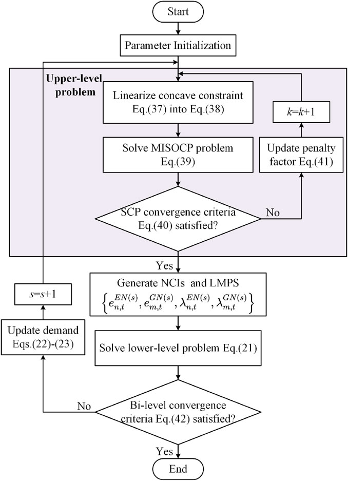
FIGURE 2. Flowchart of the bi-level interaction procedure.

4 Case studies

4.1 System description

The proposed method is tested on an IES consisting of a modified IEEE 39-bus system and a modified Belgian 20-node natural gas system, as shown in Figure 3. The detailed network parameters can be found in (Jiang et al., 2018). The system includes eleven generators (five coal-fired thermal units, three gas-turbine units, two hydro plants with total capacity of $75\mathrm{M}\mathrm{W}$, and one wind farm), four gas wells, and two compressors. The parameters of these facilities are provided in Tables 1–4. Nodes 1, 9, and 14 of the natural gas network are connected to buses 26, 32, and 36 of the electricity network via gas-turbine units, respectively. In addition, the carbon trading price is set as $30\$/\mathrm{t}\mathrm{o}\mathrm{n}$, the carbon emission allowances per unit of active power output is set as $0.648\mathrm{t}{\mathrm{C}\mathrm{O}}_2/\left(\mathrm{M}\mathrm{W}\mathrm{h}\right)$. The coefficients of utility function are adopted as $k_1=2000\$/\left(\mathrm{M}\mathrm{W}\mathrm{h}\right)$ and $k_2=10\$/{\left(\mathrm{M}\mathrm{W}\mathrm{h}\right)}^2$. SCP parameters are shown in Table 5. The 24-h electricity load, gas load, and wind power output profiles are shown in Figure 4. The proposed bi-level model is verified using the following three cases:

FIGURE 3

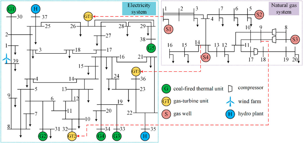
FIGURE 3. Diagram of the integrated energy system.

TABLE 1

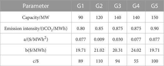
TABLE 1. Parameters of the coal-fired thermal units.

TABLE 2

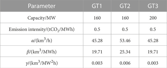
TABLE 2. Parameters of the gas-turbine units.

TABLE 3

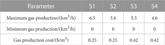
TABLE 3. Parameters of gas wells.

TABLE 4

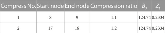
TABLE 4. Parameters of compressors.

TABLE 5

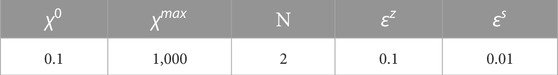
TABLE 5. Parameters of the SCP algorithm.

FIGURE 4

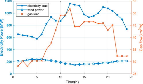
FIGURE 4. Profiles of 24-h electricity load, gas load and wind power output.

Case 1. Traditional power scheduling in the IES without carbon trading and DSM.

Case 2. Power scheduling considering carbon trading but without demand response on the user side.

Case 3. Proposed bi-level scheduling model with carbon trading policy and DSM.

4.2 Results of carbon emission intensity and LMP

In this paper, we mainly focus on the power scheduling of the electricity system. The NCIs of the 39 buses in the electricity network under two typical hours, peak hour and valley hour, are illustrated in Figure 5.

FIGURE 5

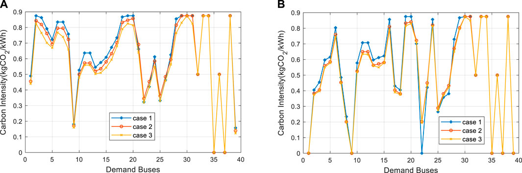
FIGURE 5. NCIs of 39 buses in (A) peak hour and (B) valley hour.

It can be observed that the average value of carbon emission intensities in peak hour is higher than those in valley hour. It is mainly because, in valley hour, wind power output is larger, and clean energy accounts for a higher proportion in the system, reducing the NCIs at the overall level. In both typical hours, Case 1 has the highest carbon intensities, followed by Case 2 and Case 3. This indicates the proposed carbon trading and DSM strategies can effectively reduce the carbon emission intensities. It should be noted that there are nodes with zero carbon intensities in the system, such as buses 35, 37 in peak hour and buses 1, 9, 39 in valley hour. This is because that they are either directly connected to zero-carbon units or their demands can be fully met by clean energy.

In peak hour, the carbon intensities in Case 2 are generally lower than those of Case 1. However, several buses, such as 21, 22, 23, 25, and 26, have higher carbon intensities than Case 1. This is due to the carbon trading in Case 2, which forces the coal-fired thermal units to reduce their output and turn to gas-turbine units with lower carbon emission intensities for power supply. As a result, although the overall carbon intensities of the system decrease, the carbon intensities of the buses near gas-turbine units increase. Compared with Case 2, the NCIs in Case 3 decrease, in which buses originally with higher carbon emissions have greater changes, like the carbon intensity of bus 8 decreases from 0.73 to 0.66. This is because the buses with higher carbon emissions would have larger adjustment of energy users’ demands through DSM, making the carbon intensity curve smoother. In valley hour, the wind power is more active, resulting in the carbon intensities of nearby buses (bus 1 and 9) remain zero in all three cases. For bus 22, due to the limited capacity of hydro power, the output increase of gas-turbine unit at bus 36 in Case 2 would change the power flow direction between bus 22 and bus 23, and there would be “carbon embedded” power flow injected to bus 22, thus improving the carbon intensity from 0 in Case 1 to 0.2 in Case 2.

The dynamic electricity prices of bus 15 in three cases are examined in this paper, as shown in Figure 6. Compared with Case 1, it is clear to see the electricity prices are raised due to the consideration of carbon emissions in Case 2. The price differences between the two cases are relatively larger in the periods when the NCI of bus 15 is high (periods 8, 18). The different LMEPs among three cases, on the other hand, can reflect the distinct NCIs in different periods. For Case 3 with the proposed DSM strategy, it can be observed that the fluctuations of price become smoother, and prices stay at around $55\$/\mathrm{M}\mathrm{W}\mathrm{h}$.

FIGURE 6

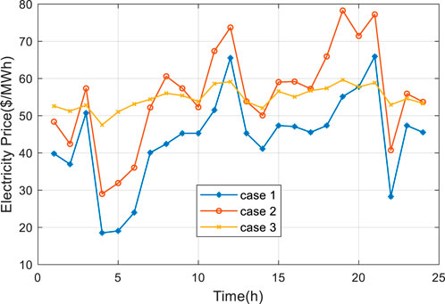
FIGURE 6. LMEPs of bus 15 in three cases.

4.3 Results of optimal scheduling

As mentioned in the case setting, in case 1, the objective function is to minimize the generation cost and the gas production cost of IES, and in case 2, carbon trading cost is added to the objective function, as shown in Eq. 7. Both case 1 and case 2 do not consider DSM, so the electricity and gas loads in these two cases will not change and we model them as single-level, which can be solved easily by the off-the-shelf commercial solver. While case 3 presents the proposed bi-level scheduling model considering carbon trading and DSM, and we can solve it through the methods shown inSection 3.

The details of the total carbon emissions and the financial conditions are shown in Table 6, where the total carbon emissions are derived from Eq. 3, the generation cost refers to ${\displaystyle \sum _t}({{\displaystyle \sum }}_{i\in {\mathrm{\Omega }}^{TU}}C\left(P_{Gi,t}\right)+{{\displaystyle \sum }}_{j\in {\mathrm{\Omega }}^{GW}}{\gamma }_{j,t}\cdot g_{j,t})$, the consumer utility and carbon trading cost can be calculated according to Eq. 24 and Eq. 9, respectively. As can be seen, cases considering carbon trading have a decided advantage in carbon emission mitigation, the total carbon emission amount in Case 2 is 19.4% lower than that of Case 1. DSM strategies can also help reduce carbon emissions, the total carbon emission amount in Case 3 is reduced by 7.7% compared to Case 2. However, the generation cost in Case 2 and Case 3 increase because more gas-turbine units with lower carbon intensities are being used, which are more expensive than coal-fired thermal units. It should be noted that the consumer utility in Case 3 has a 5.75% decrease. This is because the DSM strategy in Case 3 would motivate energy users to cut demands with high emission intensities to seek the maximum consumer surplus, which might reduce the consumer utility to some extent.

TABLE 6

TABLE 6. Carbon emissions and system cost comparison for all three cases.

Moreover, Case 2 has the highest carbon trading cost, while the carbon trading cost in Case 3 is decreased by 77.1%. The reason for this result is twofold. Firstly, there is fewer carbon emissions in Case 3, which means more carbon sources are below their emission caps so that the extra allowances that generators need to purchase are fewer. Secondly, due to the DSM, energy users in Case 3 can also sell carbon allowances to earn extra revenues in certain periods. It is obvious that whether users can obtain profits is dependent on the emission allowances allocation. When the emission allocation on the demand side is loose, the benefits of selling emission allowances would stimulate end users to participate in DSM to reduce the total carbon emissions.

The optimal scheduling results of the electricity system for all three cases on a typical day are shown in Figure 7. The hydro power remains constant in three cases because we assume that the hydro power plants are operating at their maximum power. It is evident that there is a significant reduction in the output of coal-fired thermal units from Case 1 to Case 3. The power produced by coal holds almost 54.2% of the total power generation in Case 1, and this value changes to about 50.4% in Case 2% and 44.5% in Case 3. On the contrary, the output of gas-turbine units is increasing gradually, which means under the effect of carbon trading, more GTs with lower emissions are put into use to replace the coal-fired units. The area between the generation cost and the consumer utility curves in Figure 7 represents the negative social welfare. By comparing Case 2 and Case 3, it can be seen that the proposed model has a remarkable effect on reducing the negative social welfare.

FIGURE 7

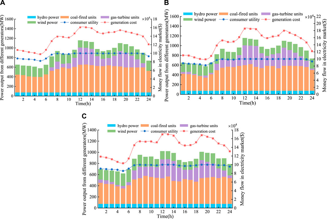
FIGURE 7. Optimal scheduling results of (A) Case 1 (B) Case 2 and (C) Case 3.

In addition, the scheduling results of the natural gas system of Case 1 and Case 3 are shown in Figure 8. Compared with Case 1, the increase of the gas-turbine units output and gas load adjustments in Case 3 result in a 17.68% increase of the gas well output, and so do the corresponding carbon emissions of the natural gas system. And the load adjustment results after DSM in Case 3 are illustrated in Figure 9. It can be observed that the electricity users tend to cut their demands in the peak hours and transfer them to the valley hours, because in valley hours, the LMEPs and NCIs are relatively low, and the demand transfer can help electricity users to optimize their cost. While the natural gas loads show the opposite trend. This is mainly because the lower level is built as a linear programming problem, when the electricity loads decrease, the natural gas users would increase their demands to raise their consumer utility, thus maximizing the whole consumer surplus.

FIGURE 8

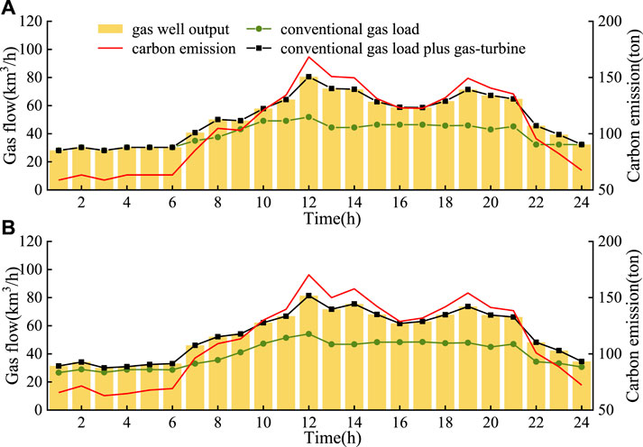
FIGURE 8. Gas network scheduling results of (A) Case 1 and (B) Case 3.

FIGURE 9

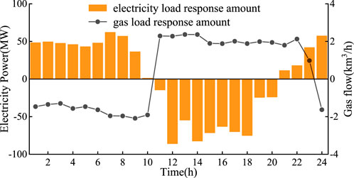
FIGURE 9. Load adjustment results after DSM.

Finally, the convergence process of SCP algorithm is presented in Figure 10. Constraint violations are significant at the beginning and decrease dramatically as the penalty factor grows. Solution with SCP is found after 6 iterations, which is feasible for the primal problem. Besides, the convergence of the bi-level interaction is illustrated in Figure 11. The demand response amount of bus 15 in the electricity network and bus 12 in the natural gas network at 13:00 in each iteration are investigated. The optimization in Case 3 can finally converge to equilibrium with 20 iterations, and the total computation time is 430s. This result verifies the feasibility of the adopted bi-level optimization model.

FIGURE 10

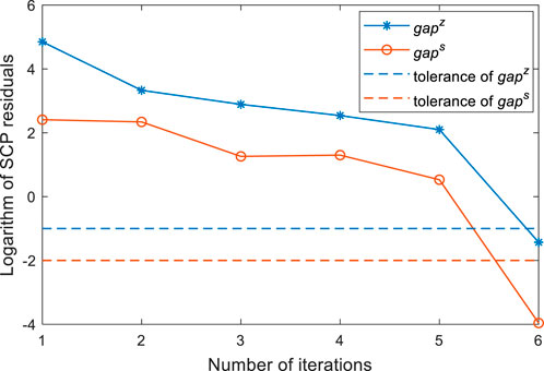
FIGURE 10. Converge curve of sequential cone programming.

FIGURE 11

FIGURE 11. Demand response amount at 13:00 in each iteration of Case 3.

4.4 Impact of the carbon trading price and gas production

The carbon trading price $\kappa$ can represent the weight of the low-carbon objective in the proposed model, and the change of carbon trading price will affect the operating state of the system. The impact of the carbon trading price on total carbon emissions and carbon trading cost in Case 3 is shown in Figure 12. Initially, when the carbon trading price is below $15\$/\mathrm{t}\mathrm{o}\mathrm{n}$, the total carbon emissions remain almost unchanged, and the carbon trading cost increases steadily with the increase of carbon trading price. In such a case, the carbon trading cost plays a minor role in the integrated objective function, and coal-fired units account for the major parts of power generation because of their cheapness. When the carbon trading price rises to $20\$/\mathrm{t}\mathrm{o}\mathrm{n}$, gas-turbine units become competitive, especially during peak hours. As a result, the total carbon emissions begin to decline significantly, and so does the cost of carbon trading. When the carbon trading price increases to around $32.5\$/\mathrm{t}\mathrm{o}\mathrm{n}$, the carbon trading cost drops to 0, which means the carbon emissions of the system is equal to the carbon allowances allocation at this point, and then environmental profits would be generated, making the carbon emissions drop rapidly. The total carbon emissions can be reduced by 40.5% with a carbon trading price of $40\$/\mathrm{t}\mathrm{o}\mathrm{n}$. However, a further increase of the carbon trading price has a slight impact on the carbon emissions when the carbon trading price is up to $45\$/\mathrm{t}\mathrm{o}\mathrm{n}$, since the output of gas-turbine units nears the maximum level, and the carbon trading cost declines slowly in proportion to the carbon trading price. This result indicates that the operating state of the IES is sensitive to the fluctuation of the carbon trading cost.

FIGURE 12

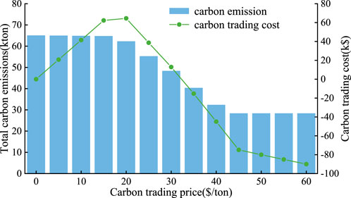
FIGURE 12. Results for different carbon trading price in Case 3.

Similar to the carbon trading price, the gas production cost also affects carbon emissions and carbon trading cost. It is evident that when the gas production cost is relatively low, the carbon emission is low as well and there would be earnings from carbon trading. The carbon emissions and carbon trading cost would rise with the gas production cost increases. It should be noted that the carbon trading price where environmental profits are generated ($32.5\$/\mathrm{t}\mathrm{o}\mathrm{n}$ in this paper) is closely related to the gas production cost. The higher the gas production cost is, the higher the carbon trading price is to obtain carbon income. Thus, the regulators can set appropriate carbon trading prices according to the gas production cost to stimulate more low-carbon energy utilization to obtain environmental revenues from both the generation side and the demand side.

5 Conclusion

This paper proposes a bi-level scheduling model to investigate the low-carbon economic operation of the electricity and natural gas IES considering DSM and carbon trading. At the upper level, an optimal energy flow model considering carbon trading at the generation side is formulated, where the SCP method is adopted to solve the relaxation gap of the gas flow equation. And the CEF model is applied to track the carbon flows accompanying the energy flows, thus the nodal carbon intensities can be obtained to clarify the emission responsibility from the perspective of end users. At the lower level, a developed demand response model is introduced, in which energy users can adjust their demands to maximize consumer surplus according to the NCIs and LMPs passed from the upper level. Case studies based on the IEEE 39-bus system and the Belgian 20-node natural gas system show that the proposed method can effectively facilitate the low-carbon operation of the IES, both the overall carbon intensities and total emissions have been significantly reduced. It should be noted that this paper adopts the centralized optimization method to model the operation of IES, but in practice the power network and the natural gas network belong to different decision-making utilities, so the decentralized optimization of electricity-natural gas IES considering DSM and carbon trading might be our future work.

Data availability statement

The raw data supporting the conclusion of this article will be made available by the authors, without undue reservation.

Author contributions

QF: methodology, software, validation, investigation, writing—original draft. JW: conceptualization, supervision, writing—review and editing. DL: conceptualization, supervision, data collection, writing—review and editing. All authors contributed to the article and approved the submitted version.

Funding

This work was supported by the National Natural Science Foundation of China–Key Program of Joint Fund in Smart Grid (U2166210).

Conflict of interest

The authors declare that the research was conducted in the absence of any commercial or financial relationships that could be construed as a potential conflict of interest.

Publisher’s note

All claims expressed in this article are solely those of the authors and do not necessarily represent those of their affiliated organizations, or those of the publisher, the editors and the reviewers. Any product that may be evaluated in this article, or claim that may be made by its manufacturer, is not guaranteed or endorsed by the publisher.

References

Borraz-Sánchez, C., Bent, R., Backhaus, S., Hijazi, H., and Hentenryck, P. (2016). Convex relaxations for gas expansion planning. Inf. J. Comput.28 (4), 645–656. doi:10.1287/ijoc.2016.0697

CrossRef Full Text | Google Scholar

Chen, S., Conejo, A., J., Sioshansi, R., and Wei, Z. (2020). Operational equilibria of electric and natural gas systems with limited information interchange. IEEE Trans. Power Syst.35 (1), 662–671. doi:10.1109/TPWRS.2019.2928475

CrossRef Full Text | Google Scholar

Cheng, Y., Zhang, N., Wang, Y., Yang, J., Kang, C., and Xia, Q. (2019). Modeling carbon emission flow in multiple energy systems. IEEE Trans. Smart Grid10 (4), 3562–3574. doi:10.1109/TSG.2018.2830775

CrossRef Full Text | Google Scholar

Cheng, Y., Zhang, N., Zhang, B., Kang, C., Xi, W., and Feng, M. (2020). Low-carbon operation of multiple energy systems based on energy-carbon integrated prices. IEEE Trans. Smart Grid11 (2), 1307–1318. doi:10.1109/TSG.2019.2935736

CrossRef Full Text | Google Scholar

Ember, (2021). The European Union and United Kingdom emissions trading system carbon market price day-by-day. Available: https://ember-climate.org/data/carbon-price-viewer/.

Google Scholar

Fang, K., Zhang, Q., Long, Y., Yoshida, Y., Sun, L., Zhang, H., et al. (2019). How can China achieve its intended nationally determined contributions by 2030? A multi-criteria allocation of China’s carbon emission allowance. Appl. Energy241, 380–389. doi:10.1016/j.apenergy.2019.03.055

CrossRef Full Text | Google Scholar

Geidl, M., and Andersson, G. (2007). Optimal power flow of multiple energy carriers. IEEE Trans. Power Syst.22 (1), 145–155. doi:10.1109/TPWRS.2006.888988

CrossRef Full Text | Google Scholar

Gu, H., Li, Y., Yu, J., Wu, C., Song, T., and Xu, J. (2020). Bi-level optimal low-carbon economic dispatch for an industrial park with consideration of multi-energy price incentives. Appl. Energy262, 114276. doi:10.1016/j.apenergy.2019.114276

CrossRef Full Text | Google Scholar

Huang, W., Zhang, N., Yang, J., Wang, Y., and Kang, C. (2019). Optimal configuration planning of multi-energy systems considering distributed renewable energy. IEEE Trans. Smart Grid10 (2), 1452–1464. doi:10.1109/TSG.2017.2767860

CrossRef Full Text | Google Scholar

International Energy Agency (Iea), (2022). Global energy review: CO2 emissions in 2021. Available: https://www.iea.org/data-and-statistics/data-product/global-energy-review-co2-emissions-in-2021.

Google Scholar

Jiang, T., Deng, H., Bai, L., Zhang, R., Li, X., and Chen, H. (2018). Optimal energy flow and nodal energy pricing in carbon emission-embedded integrated energy systems. CSEE J. Power Energy Syst.4 (2), 179–187. doi:10.17775/CSEEJPES.2018.00030

CrossRef Full Text | Google Scholar

Jiang, T., Yuan, C., Bai, L., Chowdhury, B., Zhang, R., and Li, X. (2022). Bi-level strategic bidding model of gas-fired units in interdependent electricity and natural gas markets. IEEE Trans. Sustain. Energy13 (1), 328–340. doi:10.1109/TSTE.2021.3110864

CrossRef Full Text | Google Scholar

Kang, C., Zhou, T., Chen, Q., Wang, J., Sun, Y., Xia, Q., et al. (2015). Carbon emission flow from generation to demand: A network-based model. IEEE Trans. Smart Grid6 (5), 2386–2394. doi:10.1109/TSG.2015.2388695

CrossRef Full Text | Google Scholar

Li, Y., Zou, Y., Tan, Y., Cao, Y., Liu, X., Shahidehpour, M., et al. (2018). Optimal stochastic operation of integrated low-carbon electric power, natural gas, and heat delivery system. IEEE Trans. Sustain. Energy9 (1), 273–283. doi:10.1109/TSTE.2017.2728098

CrossRef Full Text | Google Scholar

Liu, X. (2022). Research on bidding strategy of virtual power plant considering carbon-electricity integrated market mechanism. Int. J. Electr. Power Energy Syst.137, 107891. doi:10.1016/j.ijepes.2021.107891

CrossRef Full Text | Google Scholar

Lu, Z., Bai, L., Wang, J., Wei, J., Xiao, Y., and Chen, Y. (2023). Peer-to-peer joint electricity and carbon trading based on carbon-aware distribution locational marginal pricing. IEEE Trans. Power Syst.38 (1), 835–852. doi:10.1109/TPWRS.2022.3167780

CrossRef Full Text | Google Scholar

Olsen, D. J., Zhang, N., Kang, C., Ortega-Vazquez, M., and Kirschen, D. S. (2019). Planning low-carbon campus energy hubs. IEEE Trans. Power Syst.34 (3), 1895–1907. doi:10.1109/TPWRS.2018.2879792

CrossRef Full Text | Google Scholar

Paudyal, S., Cañizares, C., A., and Bhattacharya, K. (2015). Optimal operation of industrial energy hubs in smart grids. IEEE Trans. Smart Grid6 (2), 684–694. doi:10.1109/TSG.2014.2373271

CrossRef Full Text | Google Scholar

Pourakbari-Kasmaei, M., Lehtonen, M., Contreras, J., and Mantovani, J. (2020). Carbon footprint management: A pathway toward smart emission abatement. IEEE Trans. Ind. Inf.16 (2), 935–948. doi:10.1109/TII.2019.2922394

CrossRef Full Text | Google Scholar

Sun, Q., Wang, X., Liu, Z., Mirsaeidi, S., He, J., and Pei, W. (2022). Multi-agent energy management optimization for integrated energy systems under the energy and carbon co-trading market. Appl. Energy324, 119646. doi:10.1016/j.apenergy.2022.119646

CrossRef Full Text | Google Scholar

Wang, Y., Qiu, J., Tao, Y., and Zhao, J. (2020). Carbon-oriented operational planning in coupled electricity and emission trading markets. IEEE Trans. Power Syst.35 (4), 3145–3157. doi:10.1109/TPWRS.2020.2966663

CrossRef Full Text | Google Scholar

Wang, Y., Zhang, N., Kang, C., Kirschen, D., S., Yang, J., and Xia, Q. (2019). Standardized matrix modeling of multiple energy systems. IEEE Trans. Smart Grid10 (1), 257–270. doi:10.1109/TSG.2017.2737662

CrossRef Full Text | Google Scholar

Yan, M., Shahidehpour, M., Paaso, A., Zhang, L., Alabdulwahab, A., and Abusorrah, A. (2021). Distribution network-constrained optimization of peer-to-peer transactive energy trading among multi-microgrids. IEEE Trans. Smart Grid12 (2), 1033–1047. doi:10.1109/TSG.2020.3032889

CrossRef Full Text | Google Scholar

Zhang, Y., Hu, Y., Ma, J., and Bie, Z. (2018). A mixed-integer linear programming approach to security-constrained co-optimization expansion planning of natural gas and electricity transmission systems. IEEE Trans. Power Syst.33 (6), 6368–6378. doi:10.1109/TPWRS.2018.2832192

CrossRef Full Text | Google Scholar

Zlotnik, A., Roald, L., Nackhaus, S., Chertkov, M., and Andersson, G. (2017). Coordinated scheduling for interdependent electric power and natural gas infrastructures. IEEE Trans. Power Syst.32 (1), 600–610. doi:10.1109/TPWRS.2016.2545522

CrossRef Full Text | Google Scholar