Short-term PV power prediction based on the 24 traditional Chinese solar terms and adaboost-GA-BP model

High-precision, short-term power forecasting for photovoltaic systems not only reduces unnecessary energy consumption but also provides power grid security. To this end, in this paper we propose a photovoltaic short-term power forecasting model based on the division of data of the 24 traditional Chinese solar terms and the Adaboost-GA-BP model. The 24 solar terms were condensed from the laws of meteorology, phenology, and seasonal changes to adapt to agricultural times in ancient China and have become intangible cultural heritage. This article first analyzes the numerical characteristics of meteorological factors and demonstrates their close correlation with the turning points of the 24 solar terms. Second, using Standardized Euclidean Distance and Spearman’s Correlation Coefficients to analyze data similarity between the Gregorian half-months and the 24 solar terms divisions for comparative analysis purposes, it is shown that the intragroup data under the division of the 24 solar terms have a higher similarity, leading to an average decrease of 15.68%, 40.57%, 14.68%, and 14.64% in the MAE, MSE, RMSE, and WMAPE of the predicted results, respectively. Finally, based on the data derived from the 24 solar terms, the combined algorithm was compared with the Adaboost-GA-BP model and then was verified. The genetic algorithm and Adaboost were used to optimize the BP neural network algorithm in initial value assignment and neural network structure, resulting in a 23.42%, 18.12%, and 22.28% reduction in the mean values of the MAE, RMSE, and WMAPE of the predicted results, respectively. Analysis of the results show that using the Adaboost-GA-BP model based on the 24 solar terms for short-term photovoltaic power forecasting can improve the accuracy of photovoltaic power forecasting and significantly improve the predictive performance of the model.

1 Introduction

1.1 Background

Increasing depletion of non-renewable energy sources has made development of renewable energy sources a mainstream trend globally. Solar energy, being a renewable energy source with inherent characteristics such as unlimited availability, flexibility, and safety, has greatly fostered the photovoltaic (PV) industry development. In 2022, the global demand for PVs was strong, with approximately 250 GW of new installed capacity globally, a year-to-year increase of 45%. It is expected that the newly installed PV global capacity will reach 330–350 GW in 2023, which has driven great possibilities for commercial development. However, due to complex meteorological factors affecting PV power output, it also exhibits characteristics such as volatility, intermittency, and nonstationarity (Sun, 2019), which brings a series of problems for safe power grid operation. Therefore, technology for forecasting PV power output is of great significance for regulating the operational peaks, reducing unnecessary energy consumption and ensuring power system safety. High-precision prediction will also lay a foundation for research in electricity-demand management and transmission-distribution scheduling.

1.2 Literature review and motivation

Currently, research in the PV power forecasting field mainly focuses on three aspects: prediction range, prediction methods, and segmentation methods.

The prediction range is divided primarily into ultra-short-term prediction (0∼4 h), short-term prediction (0∼72 h), and medium- and long-term prediction (1 month∼1 year). Medium- and long-term predictions are generally used for power trading, siting of PV plants and benefit assessments (Cheng et al., 2012). Now, research focuses mainly on ultra-short- and short-term prediction. Ultra-short-term prediction is primarily used for PV power generation control, power quality assessment, etc. If the data sequence is stationary, at this level of minute-level prediction, the time series method has a high prediction accuracy (Reikard, 2009; Jiang et al., 2019). As for strongly volatile data, Reference (Li et al., 2021) also pointed out a hybrid deep learning model combining wavelet packet decomposition (WPD) and long short-term memory (LSTM) networks, which demonstrated superior performance in 1-h-ahead PV power forecasting with 5-min intervals. Short-term prediction is mainly used for power balance and day-ahead scheduling of the power system. The current popular method is to combine numerical weather prediction (NWP) data with power data for prediction purposes (Bacher et al., 2009; Lorenz et al., 2011; Lauret et al., 2014).

In terms of the available prediction methods, according to the physical quantity being predicted, they can be classified into indirect and direct methods (Raza et al., 2016; Das et al., 2018). The indirect method first predicts the solar irradiance and then uses neural networks or engineering formulas to predict the PV power station output. The direct method utilizes power generation historical data from the PV power station and the weather forecast data to directly predict the PV power output. According to various model categories, it can be classified into physical and statistical methods. Physical methods predict PV power generation by simulating the physical process of the electricity-generating PV components (Lorenz et al., 2011; Mandal et al., 2012; Dolara et al., 2015), which relies on studying the PV power generation equipment characteristics and does not require a large amount of sampling data. Statistical methods, on the other hand, investigates the change trend derived a large amount of historical sample data. However, it has also been noted that this physical and data-driven hybrid modeling can be used by adding physically relevant attributes to the inputs of the neural network, and that this physical and data-driven hybrid modeling is the most accurate PV power prediction technique when historical data is not available or for power prediction of new installations (Schmelas et al., 2015).

Based on the single or multiple features from the historical sample data, the data are divided into univariate and multivariate prediction methods. Univariate prediction methods generally use historical PV output power data for prediction purposes, such as time series analysis, regression analysis, and gray forecasting methods. The multivariate prediction method uses historical PV output power data as the output variable and meteorological data such as solar radiation, wind speed, and temperature as the model input variables. Common methods include artificial neural network (ANN), backpropagation (BP), deep convolutional neural network (DCNN), long short-term memory (LSTM), radial basis function (RBF), multivariate adaptive regression splines (MARS), etc., (Li et al., 2016; Wang et al., 2017; Yang et al., 2020; Zhang and Zhang, 2022; Dong et al., 2023). Among them, the BP neural network is widely used because of its strong nonlinear mapping ability (Chen et al., 2017; Meng et al., 2018; Huang et al., 2022; Liu and Huang, 2022; Wang et al., 2023). Reference (Sobri et al., 2018; Dong et al., 2023) also notes that the combined prediction model of the above methods often has better applicability and is a research topic for future power prediction. As for the problem of optimal initial value solution, there are not only simulated annealing algorithms and particle swarm optimization algorithms, but also new algorithms such as TSA and ITSA (Liu et al., 2021).

In terms of segmentation methods, dividing the dataset based on certain features to establish predictive submodels can improve the prediction accuracy. “Similar days” refers to historical load days that are similar to the predicted day in terms of weekday type, environment, weather, lunar calendar, holidays, and other factors. The theory of similar days is now widely used in the field of electricity, for purposes such as load forecasting, wind power forecasting, PV power forecasting, and so on. Reference (Li et al., 2008) notes that many similar day sample data are needed for training to obtain the variation pattern of PV power generation, so the selection of similar days will directly affect the prediction accuracy. In the selection of similar days, Reference (Shi and Li, 2016) directly divides the dataset according to four seasons, Reference (Chen et al., 2011) establishes submodels for sunny, cloudy, and rainy (snowy) day prediction, Reference (Huang, 2021) uses cloud transformation and the expectation curve method to calculate the similar days selection, and Reference (Dai et al., 2011; Yang et al., 2014) uses a self-organizing map (SOM) neural network for weather type clustering identification. In conclusion, most of the existing forecasting studies divide the dataset to build multiple adaptive forecasting models to ensure forecasting accuracy. Reference (Wang et al., 2020) proposed a day-ahead PV power forecasting model assembled by fusing deep learning modeling and time correlation principles under a partial daily pattern prediction (PDPP) framework. PDPP framework is proposed to provide accurate daily pattern prediction information of particular days, which is used to guide the modification parameters, which is a new idea for research.

For the above existing researches, there are still some issues that need to be further studied. Innovative research on the above three aspects has been ongoing, and we pondered whether we could introduce a new division, combined with high-precision prediction algorithms, to finally obtain a model suitable for short-term prediction.

1.3 Contributions

This paper is based on the PV power and meteorological factor data from three sites in the PV Power Output Dataset (PVOD), located in Hebei Province, China, which are preprocessed and then analyzed by using the Spearman correlation coefficient to correlate the meteorological factors with the power and to filter out the meteorological indicators that need further attention and analysis in this paper. Then, based on the theory of twenty-four solar terms, we propose to apply the solar calendar to the field of PV prediction. By analyzing the data, we find that the numerical characteristics of meteorological factors are closely related to changes in the twenty-four solar terms and analyze the similarity of the data within the group based on the data division of the Gregorian half month and twenty-four solar terms by calculating the Euclidean distance. Finally, through case study, we first compare and verify the data division of twenty-four solar terms and the Gregorian calendar and finally apply the combined Adaboost-GA-BP prediction model for short-term PV power prediction. It is then compared with several single prediction models to verify the short-term PV power prediction effect of the twenty-four solar terms division method and the Adaboost-GA-BP model.

Compared with the existing studies, in terms of the data set, the data obtained are from three sites instead of one site, thus avoiding some contingency; in terms of the division method, the method proposed in this paper utilizes the twenty-four seasons, a crystallization of the wisdom of the ancient Chinese people, a doctrine reflecting the laws of climate characteristics, instead of the previous research based on the data set for weather feature clustering or division into four seasons. The weather feature clustering method relies badly on the weather feature indicators, and the sub-model established is generally only applicable to the dataset under a set of weather feature indicators, while based on the twenty-four solar terms as the division, the weather feature clustering step is omitted, and the twenty-four sub-models can be divided in a simple and clear way. When divided into four sub-models according to the four seasons, compared with the division of the twenty-four solar terms, which is obviously less accurate. Then for the prediction algorithm, nowadays many pioneering artificial intelligence algorithms become prediction tools, but ignored the integration of classical algorithms such as BP neural networks, boost integration algorithms, in this paper, we find that the fusion of classical algorithms can also obtain good prediction accuracy in the example analysis.

1.4 Nomenclature

Table 1 explains some symbols that appear in the paper.

TABLE 1

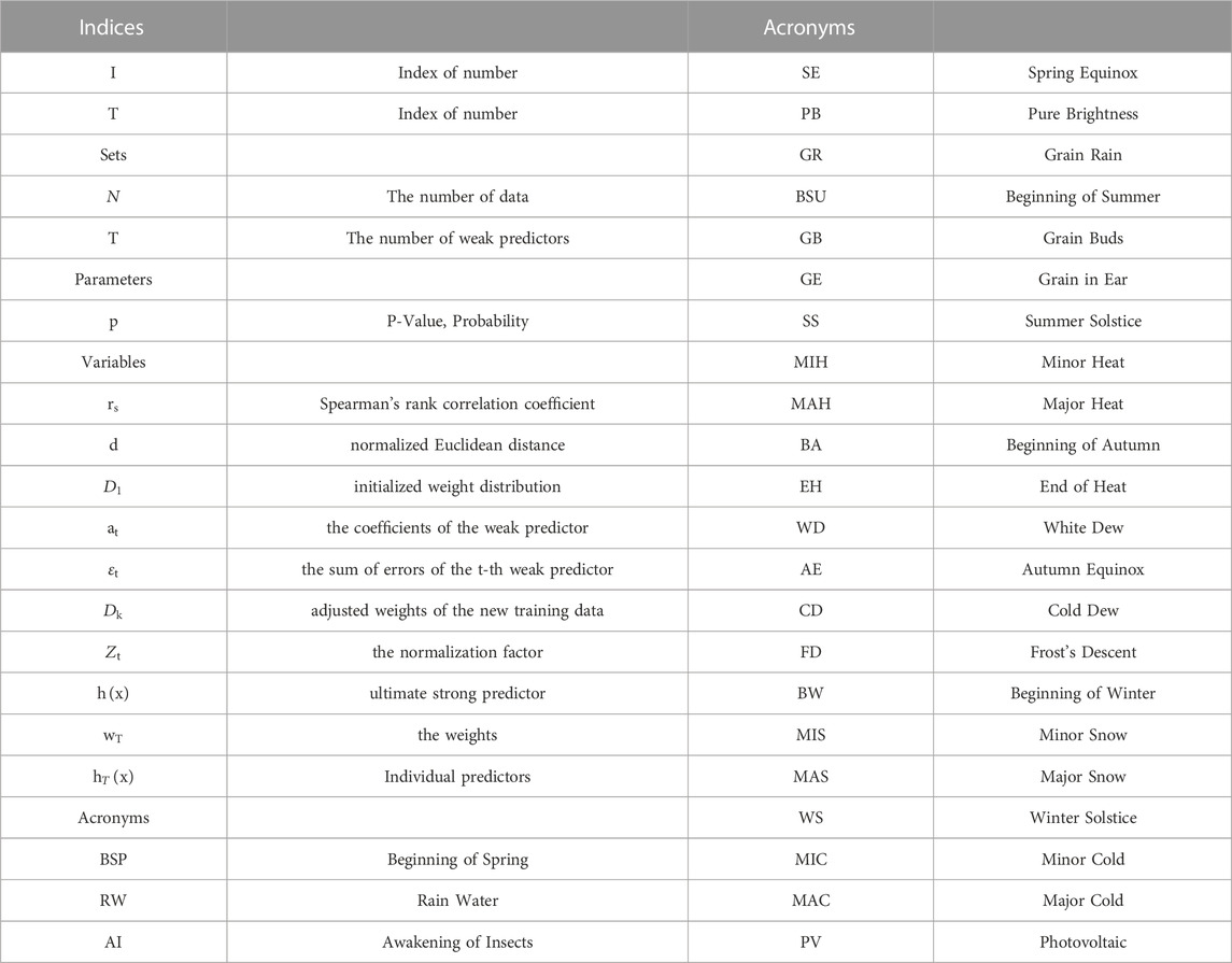
TABLE 1. Nomenclature.

2 Overview of the data

The data used in this study come from the public PVOD dataset, which includes local measurement data from ten PV sites located in Hebei, China. The PVOD dataset comprises a metadata file and data files from 10 PV sites, formatted as comma-separated values (CSV), easily accessible for browsing in Microsoft Office Excel or Notepad (Yao et al., 2021a).

This dataset is relatively comprehensive and multidimensional, with good exploratory and research value. In this study, six weather variables and PV output power from the dataset were selected. The specific variable names and definitions are shown in Table 2 (Yao et al., 2021b).

TABLE 2

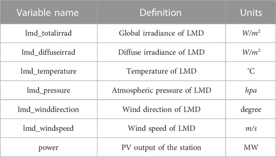
TABLE 2. Variable names and definitions of the data.

To enhance prediction accuracy, we selected three stations, noted as: station 01 located east of the station group, station 04 located in the north, and station 08 located in the southwest. Their locations are shown in Figure 1. Each station selected data from 1 July 2018, to 13 June 2019, for a total of 347 days with a time resolution of 15 min. The following is the detailed information on data acquisition and testing for three stations (Yao et al., 2021a):

FIGURE 1

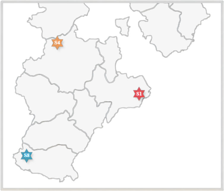
FIGURE 1. Map of the three station locations.

Three solar energy systems, located at Station01, Station04, and Station08, all boast an impressive Capacity of 20,000 kW each. They utilize PV Technology: Poly-Si and feature different panel size measurements: 1.6635 square meters for Station01, 1.6368 square meters for Station04, and 1.6335 square meters for Station08. The solar modules used in Station01 are of the LW6P60-270 type by Lightwaysolar, with a Pmax of 270 W, Vmpp of 30.52 V, and Impp of 8.86 A Station04 uses YL265P-29b modules from Yingli, offering a Pmax of 265 W, Vmpp of 30.3 V, and Impp of 8.59 A. On the other hand, Station08 employs YL265C-30b modules by Yingli, providing a Pmax of 265 W, Vmpp of 31 V, and Impp of 8.55 A.

The inverters also vary between the stations. Station01 utilizes TC500KH inverters from tbeapowe, offering a Max. DC input of 618 kW, Max. DC voltage of 1,000 V, Max. DC current of 1,344 A, and a Rated power output of 500 kW Station04 integrates SG1000 inverters by sungrowpower, featuring a Max. DC input of 560 kW, Max. DC voltage of 1,000 V, Max. DC current of 1,220 A, and a Rated power output of 1,000 kW. In contrast, Station08 employs SUN 2000-40KTL inverters from Huawei, offering a Max. DC input of 40.8 kW, Max. DC voltage of 1,000 V, Max. DC current of 23 A, and a Rated power output of 36 kW.

The layout configuration also differs: Station01 has 22 modules per string and 128 strings per inverter, Station04 has 22 modules per string and 86 strings per inverter, while Station08 features 22 modules per string and 5 strings per inverter.

The total panel number for each station is as follows: 74,000 panels for Station01, 75,680 panels for Station04, and an impressive 78,042 panels for Station08. All the arrays are tilted for maximum solar capture, with Station01 and Station08 at an array tilt of South 33° and Station04 at South 37°.

In addition, precise solar radiation measurements are taken at all stations using pyranometers. The GHI measurement is provided by TBQ-2 type pyranometers manufactured by Jinzhou Sunshine Meteorological Technology Co., Ltd., with a measurement accuracy of ±5% and a measurement range of 0–2000 W/m^2. The calibration period for GHI and DHI measurements is 2 years. The DHI measurements are obtained using the TBD-1 type pyranometer from the same manufacturer, featuring similar measurement accuracy, range, and calibration period.

Partial output power data from three stations are shown in Figure 2. After data preprocessing and application of outlier identification and detection, missing and abnormal data were fitted and interpolated, and a total of 99,936 tuples of valid data were finally selected.

FIGURE 2

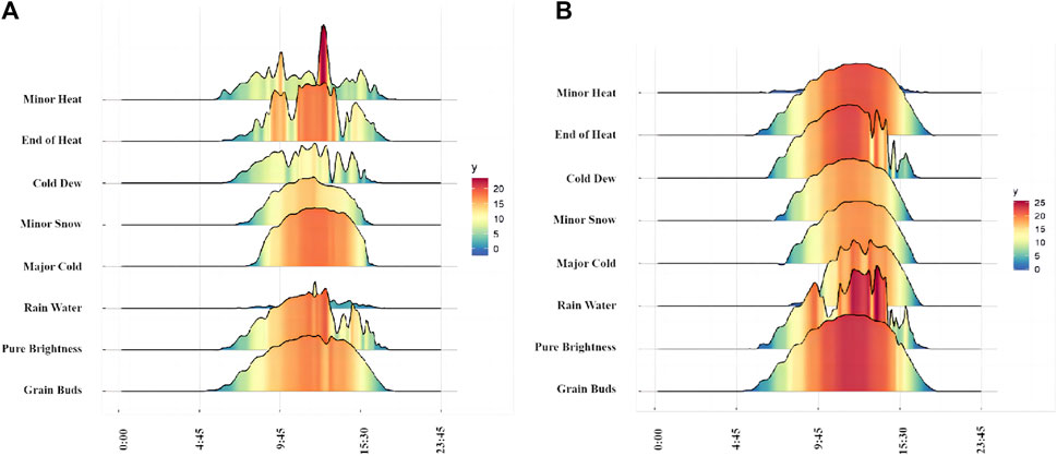
FIGURE 2. Display of partial data from Station 01 and Station 04.Y refers to the photovoltaic power output. (A) shows data from Station 01, and (B) shows data from station 04.

3 Correlation analysis of meteorological factors

The main meteorological factors associated with the study of PV power output include irradiance, temperature, humidity, air pressure, wind speed, wind direction, etc., The degree of influence of various factors on PV power generation varies significantly and by analyzing the correlation between PV power and various meteorological factors, factors with significant influence can be effectively extracted to further improve the rationality and accuracy of PV power prediction research.

Spearman’s rank correlation analysis, also known as the “rank difference method,” analyzes the correlation between variables based on rank information and calculates the difference between the number of ranks (Deng and Fang, 2019). Spearman’s correlation coefficient does not need to meet the premise that the data obeys a normal distribution and has a linear relationship between the data, so the conditions of use and application are more extensive. Spearman’s rank correlation coefficient between 2 random variables and is defined as:

${\mathbf{r}}_{\mathbf{s}}=\frac{{\displaystyle \sum _{\mathbf{i}=\mathbf{1}}^{\mathbf{n}}}\left[\left({\mathbf{R}}_{\mathbf{i}}-\frac{\mathbf{1}}{\mathbf{n}}{\displaystyle \sum _{\mathbf{i}=\mathbf{1}}^{\mathbf{n}}}{\mathbf{R}}_{\mathbf{i}}\right)\left({\mathbf{Q}}_{\mathbf{i}}-\frac{\mathbf{1}}{\mathbf{n}}{\displaystyle \sum _{\mathbf{i}=\mathbf{1}}^{\mathbf{n}}}{\mathbf{Q}}_{\mathbf{i}}\right)\right]}{\sqrt{{\displaystyle \sum _{\mathbf{i}=\mathbf{1}}^{\mathbf{n}}}{\left({\mathbf{R}}_{\mathbf{i}}-\frac{\mathbf{1}}{\mathbf{n}}{\displaystyle \sum _{\mathbf{i}=\mathbf{1}}^{\mathbf{n}}}{\mathbf{R}}_{\mathbf{i}}\right)}^{\mathbf{2}}}\sqrt{{\displaystyle \sum _{\mathbf{i}=\mathbf{1}}^{\mathbf{n}}}{\left({\mathbf{Q}}_{\mathbf{i}}-\frac{\mathbf{1}}{\mathbf{n}}{\displaystyle \sum _{\mathbf{i}=\mathbf{1}}^{\mathbf{n}}}{\mathbf{Q}}_{\mathbf{i}}\right)}^{\mathbf{2}}}}$

Where ${\mathrm{R}}_{\mathrm{i}}$ and ${\mathrm{Q}}_{\mathrm{i}}$ are the rank of the i-th $\mathrm{X}$ -value and $\mathrm{Y}$ -value, respectively, and $\mathrm{N}$ is the sample size (Wang and Chu, 2014).

The first correlation analysis was performed between the data collected at the PV site in Hebei, China. The meteorological factors to be analyzed included six factors: global irradiance, diffuse irradiance, temperature, atmospheric pressure, wind direction and wind speed. Through the large sample Kolmogorov‒Smirnov test, the significance data p-value of each variable was 0.000 at the significance level of 0.001, and the data of each variable did not conform to a normal distribution, so this paper used Spearman’s rank correlation coefficient for correlation analysis. The calculated correlation coefficients were plotted in a correlation coefficient heatmap for data visualization and analysis, as shown in Figure 3.

FIGURE 3

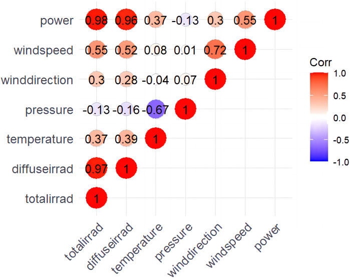
FIGURE 3. Correlation analysis of each variable.

As shown in Figure 3, there is a significant difference in the correlation between different meteorological factors and PV power generation. The correlation coefficient between PV output and global irradiance is as high as 0.98, and there is an extremely strong correlation between the two. In addition, diffuse irradiance, wind speed, and temperature also have a large impact on PV output power. Wind direction and atmospheric pressure have less influence on PV output power. Therefore, this paper selects global irradiance, diffuse irradiance, wind speed and temperature as meteorological factor indicators to focus on the analysis and utilization.

4 Twenty-four solar terms

4.1 Introduction to the principles of the twenty-four solar terms

The 24 solar terms are the crystallization of the wisdom of the Chinese working people. They are the ingenious combination and exploration of astronomy, agriculture, meteorology, customs, and other factors by ancient people. Based on changes in celestial phenomena, meteorological features, and agricultural stages, the 24 solar terms divide a year into 24 parts, including “Beginning of Spring,” “Rain Water,” “Awakening of Insects,” “Spring Equinox,” “Pure Brightness,” “Grain Rain,” “Beginning of Summer,” “Grain Buds,” “Grain in Ear,” “Summer Solstice,” “Minor Heat,” “Major Heat,” “Beginning of Autumn,” “End of Heat,” “White Dew,” “Autumn Equinox,” “Cold Dew,” “Frost’s Descent,” “Beginning of Winter,” “Minor Snow,” “Major Snow,” “Winter SolsticeWinter Equinox,” “Minor Cold,” and “Major Cold”. It is a treasure that has been precipitated throughout the long history and is a unique way for Chinese people to interpret time and understand the world. In November 2016, 24 solar terms were included in the Representative List of the Intangible Cultural Heritage of Humanity by UNESCO. As a unique system of temporal knowledge, the culture of solar terms is recognized and cherished by the world.

The 24 solar terms originated in the middle and lower reaches of the Yellow River. Later, due to their significance in agricultural production, they were adopted as a unified agricultural time system and implemented nationwide. They primarily reflect the climate characteristics of the Yellow River’s middle and lower reaches.The current commonly prescribed “24 solar terms” are determined based on the position of the sun’s return to the ecliptic. In the annual movement of the sun, starting from 0 degrees of celestial longitude when the sun is directly overhead at the equator, each 15-degree movement constitutes a solar term. Therefore, the entire trajectory is divided into 24 equal parts, as shown in Figure 4. The famous astronomer Zixin Zhang of the Northern Wei and Northern Qi dynasties in China discovered the unevenness of the sun’s apparent motion in approximately 570 AD. Specifically, this was expressed as “the sun moves slower after the Spring Equinox and faster after the Autumn Equinox”, which is now recognized in modern astronomy as a manifestation of the variation in the sun’s orbital speed. Using similar methods to divide the prediction training sets of power, one can effectively demonstrate the laws of the sun’s speed changes over the year and better reflect the characteristics of each solar term.

FIGURE 4

FIGURE 4. View of the Sun’s path in the orbit for the 24 Solar Terms.

In ancient China, people invented the “gnomon” to measure changes in the length of shadows during the Sun’s periodic movements. They discovered two extremes, being the Winter Solstice when shadows are longest and the Summer Solstice when shadows are shortest, providing two important scales for the ancient Chinese time system. Following the observation of changes in the sun, ancient people further identified two special days that divide day and night in a year: the Spring Equinox and the Autumn Equinox (Liu, 2017). In the middle of the spring and autumn period, with the improvement of gnomon sun-measuring technology and the development of astronomy, the four solar terms of the Beginning of Spring, Summer, Autumn and Winter were determined. During the Qin and Han dynasties, the 24 solar terms were fully established, and the names and order of the 24 solar terms described in An Liu’s book Huainan Zi remain used to this day (Sui and Zhang, 2020). During the process from the initial creation to the completion of the twenty-four solar terms, we can clearly see the important role played by the sun movement and irradiation. As recorded in the book Shang Shu · Yaodian, “When the day is not too long or too short, the middle star is Alphard, which is the day of the Spring Equinox; the longest daytime period, when the central star is Antares, is the Summer Solstice; when the night is not too long or too short, the middle star is Emptiness, which is the Autumn Equinox; when the day is shortest, the middle star is Hairy Head, which is the Winter Solstice,” the division of solar terms depends on the position of the sun, the time of sunrise, and other factors, and must be closely related to the irradiation size and length. In China, there are also widely circulated folk sayings such as “Rainy on the day of “Li Chun” (Beginning of Spring), wet and damp until “Qing Ming” (Pure Brightness),” “Rainfall at “Li Xia” (Beginning of Summer) and “Xiao Man” (Grain Buds), competing with each other,” “Hot as fire during “Mang Zhong” (Grain in Ear), raining heavily at “Xia Zhi” (Summer Solstice),” which reflect the relationship between the 24 solar terms and weather conditions, further demonstrating the consistency between the solar terms and factors such as radiation and temperature. From the analysis performed above, it can be seen that the 24 solar terms can effectively divide a year according to factors such as weather, seasons, and temperature, especially with obvious correlation features with solar radiation and temperature.

The 24 solar terms are not only an excellent traditional culture but also a tool full of wisdom. From ancient times to the present, the 24 solar terms have been widely used in agricultural activities to guide farmers in various agricultural production labor. As the cultural influence of the 24 solar terms gradually spreads worldwide, its scope of application is also becoming increasingly broader. Currently, scholars have already applied the 24 solar terms to multiple fields, such as stock prediction (Zhou et al., 2021), load prediction (Xie and Hong, 2018), and wind power generation prediction (Han et al., 2020).

Introducing meteorological features into PV power prediction can significantly improve its scientific and predictive accuracy. The main factors that affect PV power, such as irradiance and temperature, are closely related to the 24 solar terms. Therefore, this article innovatively applies the 24 solar terms to the field of PV power prediction, exploring the close relationship between the 24 solar terms and multiple factors such as temperature and irradiance. By utilizing the scientific and practicality of dividing data into 24 solar terms, a highly innovative method for predicting PV power is provided.

4.2 Analysis of numerical characteristics of meteorological factors

The 24 solar terms are closely related to changes in temperature and precipitation, so it is necessary to analyze the numerical characteristics and meteorological factor variations in the 24 solar terms. We observe the numerical characteristics of global irradiance, diffuse irradiance, temperature, and wind speed under the division of the 24 solar terms by plotting. For global irradiance, diffuse irradiance, and temperature meteorological factors, we can select the maximum value within an interval. However, since wind speed is subject to rapid changes over time, selecting the maximum value within an interval is not meaningful. Therefore, we analyze it by selecting the mean value within an interval. Figures 5A, B show the maximum global irradiance and diffuse irradiance values for the 22 solar terms at site 1 in the dataset, respectively. Both global and diffuse irradiance reach their peaks around the Beginning of Autumn, followed by a sharp decline, reaching their minimum near the Beginning of Winter. From the beginning of Spring, both irradiance types enter a period of rapid growth, and then they enter a slower growth phase starting from the Beginning of Summer. Figure 5C shows the variation in temperature with solar terms, which is roughly consistent with the variation pattern of irradiance. Figure 5D shows the variation in wind speed with solar terms. By selecting the mean values, it can be observed that the wind speed decreases after the Beginning of Autumn, reaches its minimum near the beginning of winter, fluctuates greatly after the Beginning of Spring, and sharply increases to its highest point after a sudden drop.

FIGURE 5

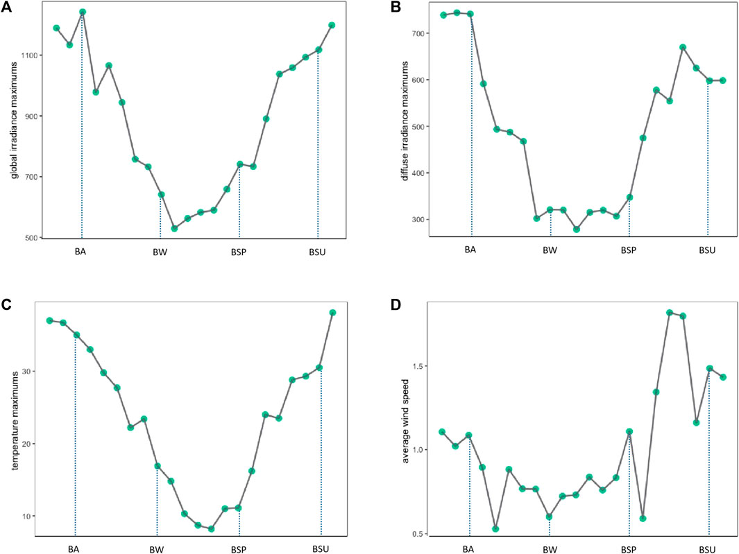
FIGURE 5. Four types of data for Station 01. (A) Global irradiance maximums, (B) Diffuse irradiance maximums, (C) Temperature maximums, (D) Average wind speed.

Analysis of the global irradiance, diffuse irradiance, temperature, and wind speed meteorological factors at Site 4 indicates that the seasonal changes in global irradiance (Figure 6A), diffuse irradiance (Figure 6B), and temperature (Figure 6C) are broadly consistent with the trends observed at other sites. However, wind speed (Figure 6D) shows significant variability with no clear pattern. Nevertheless, based on the above analysis, to some extent, certain turning points of the 24 solar terms can reflect the seasonal changes and numerical characteristics of global irradiance, diffuse irradiance, temperature, and wind speed meteorological factors.

FIGURE 6

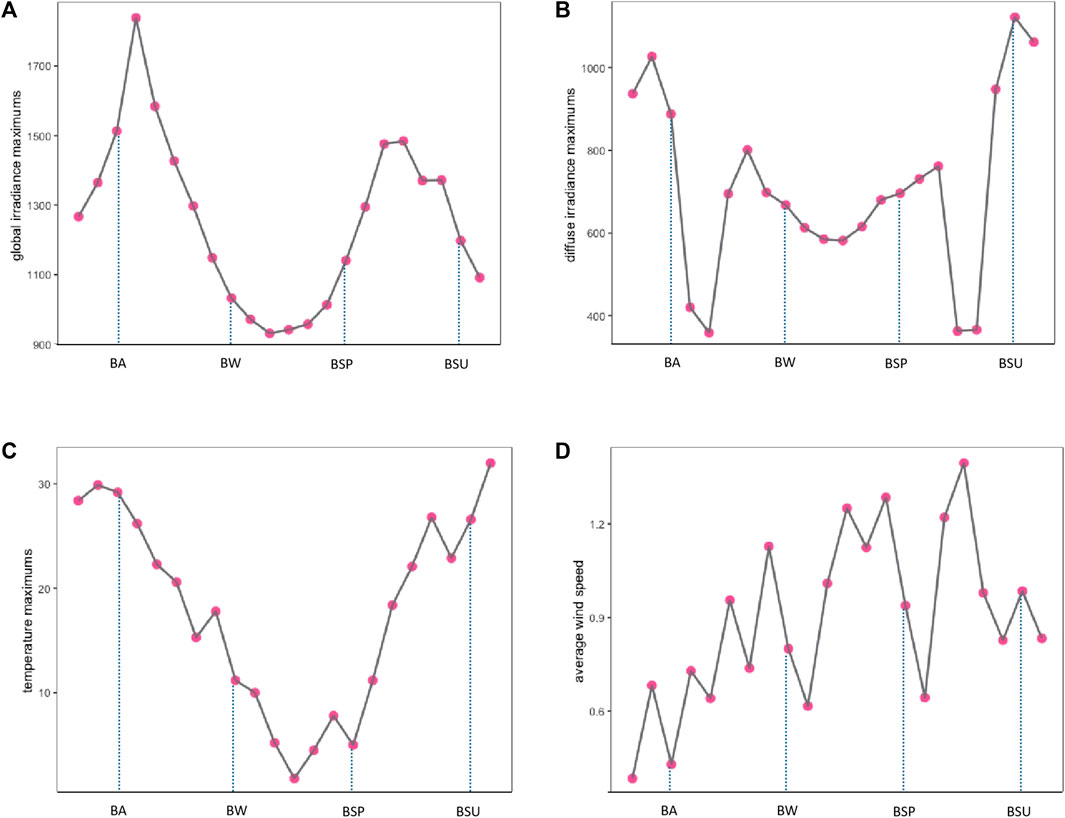
FIGURE 6. Four types of data for Station 04.(A) Global irradiance maximums, (B) Diffuse irradiance maximums, (C) Temperature maximums, (D) Average wind speed.

4.3 Sample similarity between solar calendar and gregorian calendar

To better illustrate the rationality of using the 24 solar terms to divide the dataset, the similarity of the dataset in two cases, grouped by calendar date and grouped by solar terms, is examined separately in this paper. The similarity measure is an important way to measure the degree of similarity between two samples. Among them, the Euclidean distance is the most easily understood and commonly used similarity metric, which is defined in Euclidean space, while the standardized Euclidean distance (SED) makes for a more consistent measure of distance by normalization and eliminates the effect of dimensionality. The normalized Euclidean distance between two n-dimensional vectors $\mathrm{\alpha }$ (${\mathrm{x}}_1$, ${\mathrm{x}}_2$, …, ${\mathrm{x}}_{\mathrm{n}}$), $\mathrm{\beta }$ (${\mathrm{y}}_1$, ${\mathrm{y}}_2$, …, ${\mathrm{y}}_{\mathrm{n}}$)is calculated as follows:

$\mathbf{d}=\sqrt{{\sum }_{\mathbf{i}=\mathbf{1}}^{\mathbf{n}}\frac{{\left({\mathbf{x}}_{\mathbf{i}}-{\mathbf{y}}_{\mathbf{i}}\right)}^{\mathbf{2}}}{{\mathbf{s}}_{\mathbf{i}}}}$

In this paper, the datasets of the two sites were divided into groups according to the 24 solar terms, and only 22 groups were retained from the Minor Heat to the Grain Buds due to data limitations. The SED and Spearman’s correlation coefficients of each variable were calculated for each of the two sites at the same time, and the mean values were found. Similarly, the datasets of the two stations were divided into groups of 15 days according to the calendar date, and the corresponding 22 groups were divided. The SED and Spearman’s correlation coefficients of each variable for each of the two stations in the same period were calculated separately, and the mean values were found. A visual plot of the correlation and SED for each of the two indicators grouped under the 24 solar terms and grouped under the Gregorian dates is shown in Figure 7A, B.

FIGURE 7

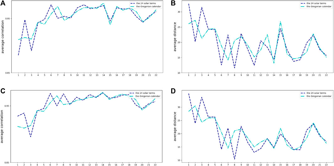
FIGURE 7. Comparison of Spearman correlation coefficient and SED power and global irradiance data. (A) Spearman correlation coefficient of power data, (B) SED of power data (C) Spearman correlation coefficient of global irradiance data, (D) SED of global irradiance data.

The following analysis can be performed from the power data correlation and the SED line graph. The closer the average correlation value is to 1, the stronger the correlation of the power data between the three sites and the higher the similarity within the dataset. As seen from the figure, the correlations of the datasets grouped by the 24 solar terms (treatment 1) corresponding to the four solar terms 1, 3, 7, and 19 (i.e., Minor Summer, Beginning of Autumn, Cold Dew, and Pure Brightness) are significantly lower than those grouped by calendar dates (treatment 2), while the correlations of treatment 1 in the remaining solar terms show significantly better results than, or are generally consistent with, those of treatment 2. The average distance metric is a look-ahead metric, and the smaller the value of the distance metric, the closer the distance of the power data between the three sites and the higher the similarity within the dataset. As seen from the figure, the distance values corresponding to treatment 1 were significantly lower than those of treatment 2 at the 2nd, 6th, 8th, 11th, 17th, and 18th (i.e., Major Heat, Autumn Equinox, Frost’s Descent, Major Snow, Awakening of Insects, and Spring Equinox) and reached the minimum value at Frost’s Descent. Although the distance index showed fluctuating changes on both treatments, on the whole, treatment 1 was able to achieve the effect of reducing the distance, which means increasing the similarity, on most of the solar terms.

For the global irradiance data, is shown in Figures 7C, D, 8 the correlations for treatment 1 were significantly better than or generally consistent with treatment 2 for all solar terms, except for the significant inflection points for 2nd, 7th, and 19th solar terms (i.e., Major Summer, Cold Dew, and Pure Brightness). It can also be seen from the mean distance plots that the distances of treatment 1 were significantly better than, or basically the same as, treatment 2 in all the other solar terms, except for the 1st, 3rd, 7th and 19th (i.e., Minor Summer, Beginning of Autumn, Cold Dew, and Pure Brightness) solar terms, which were significantly higher than treatment 2 and reached the minimum value at the Frost’s Descent.

FIGURE 8

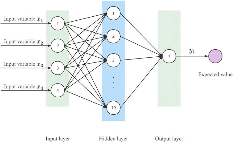
FIGURE 8. Topological structure diagram of the BP neural network.

This shows that the global irradiance and power data are more similar according to the 24 solar terms, which can ensure a better training effect when substituting into the model prediction and help to improve the prediction accuracy of PV power. Therefore, the 24 solar term data classification method provided in this paper has good applicability and innovation in PV power prediction, and combined with the Adaboost-GA-BP model with an excellent prediction effect constructed in this paper, it can yield more accurate PV power prediction results.

5 Models and methods

After dividing photovoltaic power output data into 24 solar terms, a method is needed for short-term power prediction. This paper chooses the Adaboost-GA-BP model to predict the short-term power of the PV system. Based on the powerful linear mapping ability of the BP neural network, this model optimizes its initial weights using a genetic algorithm and optimizes its network structure using the Adaboost algorithm, thereby improving the prediction accuracy and the generalization ability of the BP neural network and overcoming its tendency to fall into local optimal solutions.

5.1 Backpropagation neural network

ANNs are widely used in various fields for prediction purposes. As PV output power is mostly affected by meteorological factors which have strong randomness and uncertainty, increasing the difficultness to fully clarify the impact of each meteorological factor on the power. However, ANNs can complete input‒output mapping even when the understanding of variables is insufficient, and they have strong mapping ability. In practical applications of neural networks, 80% to 90% of them use a BP neural network and its optimization algorithm (Huang, 2008). The BP neural network stores information in a distributed manner, has strong environmental adaptability and self-learning ability, can accurately approximate nonlinear mappings, and therefore has good robustness and fault tolerance.

The BP neural network simulates the information transmission between biological neurons and consists of an input layer, a hidden layer, and an output layer. Its basic structure is shown in Figure 9.

FIGURE 9

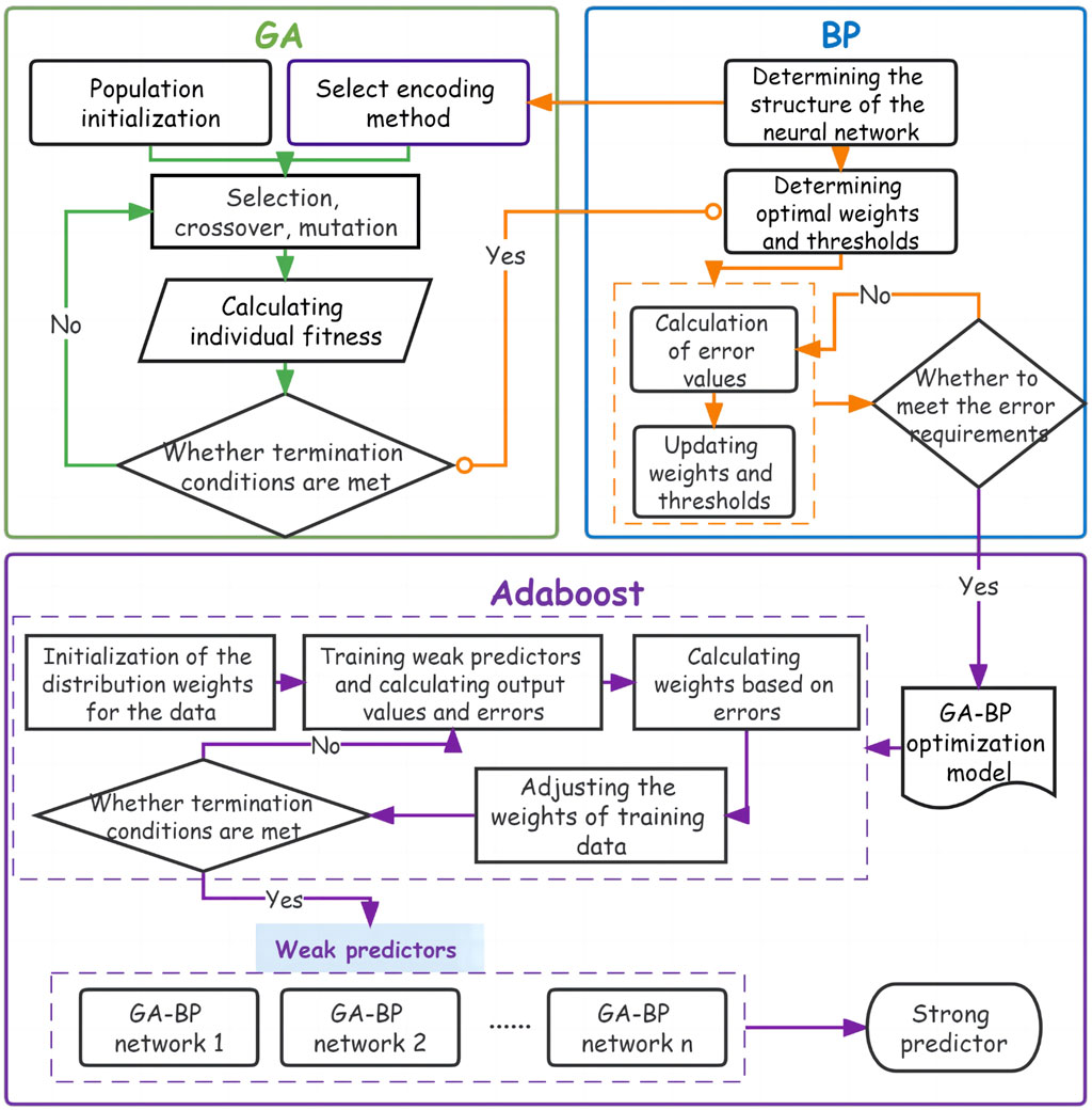
FIGURE 9. Flow chart of the Adaboost-GA-BP algorithm.

The BP neural network is a multilayer feedforward artificial neural network based on the gradient’s steepest descent method that uses the BP algorithm to effectively improve the prediction accuracy. However, it still faces issues such as easily falling into local minima and having difficulty determining network generalization capabilities, which can be resolved by optimizing weight initial values and network structure. According to the Kolmogorov theorem, a three-layer BP neural network with one hidden layer can approximate any nonlinear continuous function on a closed set with arbitrary precision (Huang, 2008). The number of hidden layer nodes, maximum iteration times and learning rate of the BP neural network used in this paper are 19,1000 and 0.1, respectively.

5.2 GA-BP

Genetic algorithms originate from research on natural and artificial adaptive systems (Sampson, 1976). It is an adaptive global optimization probabilistic search algorithm formed by simulating the genetic and evolutionary process of organisms in the natural environment (Fu and Zhao, 2010). Based on Darwin’s theory of evolution, the survival ability of organisms in a new environment depends on their adaptability. By integrating the selection, crossover, and mutation mechanisms in genetic and evolutionary processes, the genetic algorithm retrieves the optimal solution from a population of multiple individuals, with the fitness function value directly derived from the change in the objective function as the standard for seeking the optimal solution. Therefore, the genetic algorithm is an applicable method to global optimization, but its randomness leads to a poor local convergence ability.

The BP neural network is an effective method for updating the neural network weights based on the gradient of the loss function with respect to the network parameters. Its backpropagation is more suitable for training nonlinear relationship data, making it suitable for training complex meteorological data related to photovoltaics. However, it has the issues of easily getting stuck in local optima and overfitting. On the other hand, genetic algorithms can perform global, complex, and multimodal optimization, complementing the shortcomings of the BP neural network. Therefore, the GA-BP algorithm is chosen for further research.

Genetic algorithms are mainly used to optimize the initial weights and thresholds of BP neural networks. The genetic algorithm and the BP neural network complement each other well in the process of searching for the optimal solution, with the genetic algorithm optimizing situations where the BP neural network is prone to becoming stuck in local optimal solutions. The best parameters for this model were obtained through multiple experiments, where the evolutionary generation, population size, crossover probability, and mutation probability were 19,1000,0.8, and 0.1, respectively.

5.3 Adaboost-GA-BP

It is difficult in practice to avoid the phenomenon of overfitting by using a single model. The Adaboost algorithm uses the idea of combining models to improve the prediction accuracy and generalization ability of the model by using multiple GA-BP neural networks as weak classifiers and continuously upgrading them to strong learners. (Kar and Melody, 1992; Tian and Mao, 2009; Yang et al., 2023). The steps for building the Adaboost-GA-BP model are as follows:

1. Construction of the neural network: Determination of the basic structure of the neural network and partitioning of the dataset;

2. Determine the initial network value: Training the neural network with GA to output the initial weights and thresholds of the BP neural network that meet the accuracy requirements by initializing the populations and performing genetic operations such as crossover and mutation;

3. Initialize the distribution weights of the data: Initialize the weight distribution of the training data as:

${\mathbf{D}}_{\mathbf{1}}=\left(\frac{\mathbf{1}}{\mathbf{N}},\frac{\mathbf{1}}{\mathbf{N}},\cdots ,\frac{\mathbf{1}}{\mathbf{N}}\right)$

4. Train the weak predictors: For the t-th weak predictor, train the GA-BP neural network with the training set, calculate the output value $h_t$, and calculate the sum of errors ${\epsilon }_t$ based on the actual values;

5. Calculate the coefficients of the weak predictor: Calculate the weight corresponding to each weak predictor based on the sum of its errors $\epsilon$ as:

${\mathbf{a}}_{\mathbf{t}}=\frac{\mathbf{1}}{\mathbf{2}}\mathbf{ln}\frac{\mathbf{1}-{\mathrm{\epsilon }}_{\mathbf{t}}}{{\mathrm{\epsilon }}_{\mathbf{t}}}$

6. Adjust the weight distribution of the data: the weights of the new training data are adjusted according to the updated weights $a$:

${\mathbf{D}}_{\mathbf{k}+\mathbf{1}}\left(\mathbf{i}\right)=\frac{{\mathbf{D}}_{\mathbf{k}}\left(\mathbf{i}\right){\mathit{e}}^{-{\mathbf{a}}_{\mathbf{t}}{\mathbf{y}}_{\mathbf{i}}{\mathbf{h}}_{\mathbf{t}}\left({\mathbf{x}}_{\mathbf{i}}\right)}}{{\mathbf{Z}}_{\mathbf{t}}}$

where ${\mathrm{Z}}_{\mathrm{t}}$ is the normalization factor that makes ${\displaystyle \sum _{\mathrm{i}=1}^{\mathrm{N}}}{\mathrm{D}}_{\mathrm{k}+1}\left(\mathrm{i}\right)=1$;

7. Combine into strong predictors: Keep repeating the above steps until the iteration coefficients reach T times to stop and determine the weights ${\mathrm{w}}_{\mathrm{t}}$. The weak predictor obtained from the training combines the strong predictor:

$\mathbf{h}\left(\mathbf{x}\right)={\mathbf{w}}_{\mathbf{1}}{\mathbf{h}}_{\mathbf{1}}\left(\mathbf{x}\right)+{\mathbf{w}}_{\mathbf{2}}{\mathbf{h}}_{\mathbf{2}}\left(\mathbf{x}\right)+\cdots {\mathbf{w}}_{\mathbf{T}}{\mathbf{h}}_{\mathbf{T}}\left(\mathbf{x}\right)$

Due to the limitations of BP neural network, this paper adds genetic algorithm and ADABOOST method to optimize the original model in terms of initial value assignment and neural network structure respectively, thus increasing the complexity of the model. In the empirical analysis, the best parameter model obtained through repeated testing reflects the strong fitting and forecasting ability of the model, and its parameter values also reflect the complexity of the model. However, the complexity of the model is suitable for practical problems and data, which ensures the stability of the model and makes the model have the best prediction effect. Based on the complexity of the model, the size of the data, the selection of computing software and other factors, the training time of the model in this paper is about 20 min, which is consistent with the large data set and the network structure of the model adopted in this paper.

5.4 Model evaluation index

To test the accuracy of the model prediction results, and considering that the value of some of the data applied in this paper is zero, four indicators, mean absolute error (MAE), mean square error (MSE), root mean square error (RMSE), and weighted mean absolute percentage error (WMAPE), are selected for evaluation in this paper. The specific calculation is as follows:

$\mathbf{M}\mathbf{A}\mathbf{E}=\frac{\mathbf{1}}{\mathbf{n}}{\displaystyle \sum _{\mathbf{i}=\mathbf{1}}^{\mathbf{n}}}\left|{\mathbf{y}}_{\mathbf{p}\mathbf{i}}-{\mathbf{y}}_{\mathbf{i}}\right|$

$\mathbf{M}\mathbf{S}\mathbf{E}=\frac{\mathbf{1}}{\mathbf{n}}{\displaystyle \sum _{\mathbf{i}=\mathbf{1}}^{\mathbf{n}}}{\left({\mathbf{y}}_{\mathbf{p}\mathbf{i}}-{\mathbf{y}}_{\mathbf{i}}\right)}^{\mathbf{2}}$

$\mathbf{R}\mathbf{M}\mathbf{S}\mathbf{E}=\sqrt{\frac{{\displaystyle \sum _{\mathbf{i}=\mathbf{1}}^{\mathbf{n}}}{\left({\mathbf{y}}_{\mathbf{p}\mathbf{i}}-{\mathbf{y}}_{\mathbf{i}}\right)}^{\mathbf{2}}}{\mathbf{n}}}$

$\mathbf{W}\mathbf{M}\mathbf{A}\mathbf{P}\mathbf{E}=\frac{{\displaystyle \sum _{\mathbf{i}=\mathbf{1}}^{\mathbf{n}}}\left|{\mathbf{y}}_{\mathbf{p}\mathbf{i}}-{\mathbf{y}}_{\mathbf{i}}\right|}{{\sum }_{\mathbf{i}=\mathbf{1}}^{\mathbf{n}}{\mathbf{y}}_{\mathbf{i}}}$

where ${\mathrm{y}}_{\mathrm{p}\mathrm{i}}$ is the predicted power value of the i-th sample, ${\mathrm{y}}_{\mathrm{i}}$ is the actual power value of the i-th sample, and n is the total number of samples.

6 Results

6.1 Processing of the twenty-four solar term divisions of data

To verify the rationality of dividing the data according to the twenty-four solar terms, we divided the data from 1 July 2018, to 13 June 2019, for a total of 347 days, according to both the Gregorian calendar and the twenty-four solar terms. To ensure the completeness of the data within each solar term, the total data were divided into 22 groups, from Minor Heat to Grain Buds of the following year. The full name and abbreviation of each group are Minor Heat (MIN), Major Heat (MAH), Beginning of Autumn (BA), End of Heat (EH), White Dew (WD), Autumn Equinox (AE), Cold Dew (CD), Frost’s Descent (FD), Beginning of Winter (BW), Minor Snow (MIS), Major Snow (MAS), Winter Equinox (WE), Minor Cold (MIC), Major Cold (MAC), Beginning of Spring (BSP), Rain Water (RW), Awakening of Insects (AI), Spring Equinox (SE), Pure Brightness (PB), Grain Rain (GR), Beginning of Summer (BSU), and Grain Buds (GB).

The ratio of the training set to the test set is 8:2. Among them, for the two division methods of the twenty-four solar terms and the Gregorian calendar, the first 80% is selected as the training set according to the time sequence, and the last 20% is selected as the test set. Then, the overlapping solar term day of the two sets is chosen as the detection day for further analysis. It should be noted that due to the 24 solar terms not being evenly distributed and some data being missing, the data quantity varies for each group, with an average of approximately 4,351 entries. Four input features, including global irradiance, diffuse irradiance, wind speed, and temperature, are used as the model inputs; the predicted PV power output at each future time point is the output feature. To highlight the prediction performance, both groups use the day of the solar term as the validation day and present the results in a visualized manner.

6.2 Prediction results of the division point between 24 solar terms and the gregorian calendar

After dividing the dataset in the above way, this paper first applies the Adaboost-GA-BP model to the grouping of 24 solar terms and the Gregorian calendar for comparison experiments, and the prediction errors MAE, MSE, RMSE and WMAPE obtained from the two divisions are shown in Table 3.

TABLE 3

TABLE 3. 24 solar terms and Gregorian calendar division error comparison.

From the data in the table, it can be seen that 16 solar terms grouped by 24 solar terms have better prediction errors than those grouped by the Gregorian calendar (*). By analyzing the mean values of the data, the division according to the 24 solar terms led to a decrease in the MAE, MSE, RMSE and WMAPE by 15.68%, 40.57%, 14.68% and 14.64%, respectively, and the overall prediction effect of the 24 solar term division was better than that of the Gregorian calendar division, which was due to the 24 solar term division data ability to better extract the similarity between the data, it and also had a better fitting effect.

From the MAE index analysis, the error in the case of grouping by 24 solar terms can be reduced by 60.1%, 51.4%, 48.6%, 33.3% and 32.2% for White Dew, Frost’s Descent, Minor Cold, Cold Dew and Winter Solstice, respectively, compared with the grouping by Gregorian calendar. In terms of the MSE index, grouping by 24 solar terms can reduce the errors of White Dew, Minor Cold, Frost’s Descent, Winter Solstice and Major Snow by 81.8%, 76.1%, 66.9%, 59.8%, and 39.7%, respectively, compared to grouping by the Gregorian calendar. From the RMSE index analysis, the errors of White Dew, Minor Cold, Frost’s Descent, Winter Solstice and Cold Dew can be reduced by 57.4%, 51.1%, 42.5%, 36.6% and 22.4%, respectively, in the case of grouping by 24 solar terms compared to grouping by the Gregorian calendar. From the WMAPE index analysis, the errors of Minor Cold, White Dew, Beginning of Winter, Rain Water and Frost’s Descent decreased by 56.2%, 40.8%, 37.3%, 33.1% and 28.9%, respectively. From the error data, it can be seen in most cases that the 24 solar term division method can significantly reduce the prediction error of PV output power.

As seen in Figure 10A of the White Dew real data and the predicted results for the two divisions, the predicted results are closer to the actual power values in the case of grouping by 24 solar terms than in the case of grouping by the Gregorian calendar. In particular, the predicted power values under the 11:00–16:00 part grouped by the Gregorian calendar showed several significant deviations from the true values, while the predicted power values under the 24 solar terms were consistent with the true power values, with small differences.

FIGURE 10

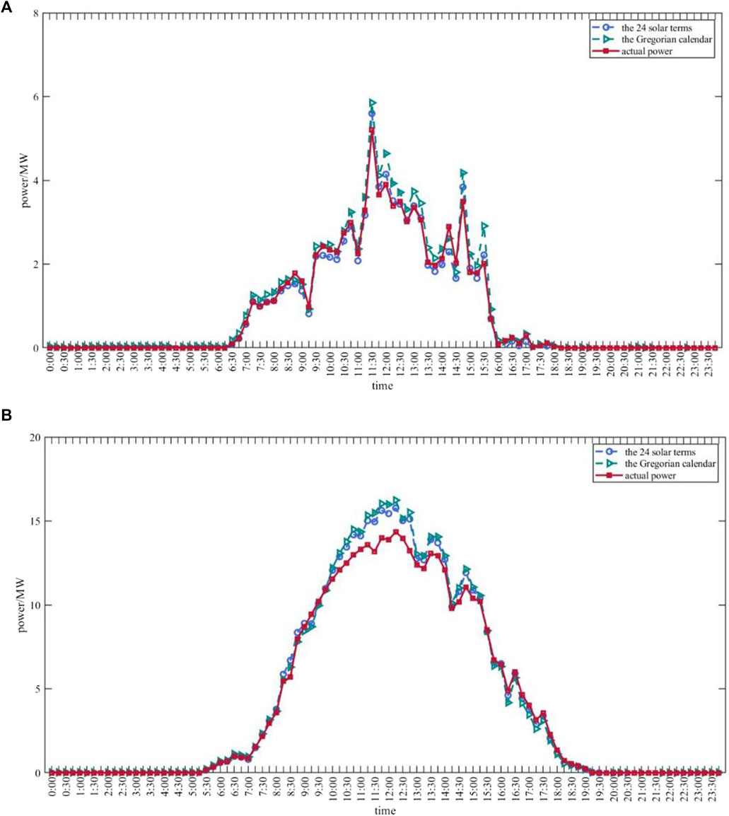
FIGURE 10. The prediction results of the photovoltaic output power of the White Dew (A) and Frost’s Descent (B) based on the division of the 24 solar terms () and the Gregorian calendar () were compared with the original data ().

Similarly, a comparison of the predicted results for Frost’s Descent is plotted in Figure 10B, from which it can be seen that the results under the grouping by the Gregorian calendar deviate more from the true values, especially between 10:00 and 13:00 h. Although there are some differences between the prediction results and the real power under the grouping of 24 solar terms, the prediction error is smaller than that of the other grouping method, which has a better prediction effect.

From the plotting and analysis of the prediction results according to the specific solar terms listed above, it can be seen that the prediction results under the grouping of 24 solar terms are mostly better than the prediction results under the grouping of the Gregorian calendar, which can better match the actual value trends and the value magnitudes. However, there are cases where the grouping of solar terms does not optimize the prediction results, which may be related to the lack of internal similarity of the data corresponding to the solar term. For example, both the correlation and distance data corresponding to the Beginning of Autumn indicate that the similarity between the data under the grouping of this solar term by the Gregorian calendar is significantly higher, and its corresponding prediction effect also indicates that the prediction effect under the grouping of the Gregorian calendar is better. The similarity between the two treatments for White Dew and Frost’s Descent is smaller, or the similarity is significantly higher when grouped by 24 solar terms than when grouped by the Gregorian calendar, and their corresponding prediction values also show that grouping by 24 solar terms can optimize the prediction effect.

Therefore, based on the feature that the internal similarity of data significantly affects the training and the prediction effects of the model, the data division method of 24 solar terms proposed in this paper, in most cases, can make the internal similarity of each group of data higher, and the error results also show that this data division method can optimize 66.67% of the solar terms, which has better data division and prediction accuracy than the traditional grouping by Gregorian calendar in practical applications. It has a significant advantage in optimizing the prediction effect and has a wide scope for promotion and research.

6.3 Predictive results and comparative validation of the adaboost-ga-bp model

To further validate the algorithmic performance of the Adaboost-GA-BP model under the division of the 24 solar terms, four sets of comparative experiments were conducted with the above parameters by setting the Adaboost-GA-BP model along with the BP, Adaboost-BP, and GA-BP models. The predictive results were compared, and the MAE, RMSE, and WMAPE error values of the models were obtained, shown in Table 4. Compared to the BP neural network, the average predictive errors of the Adaboost-GA-BP model on the 22 data points were reduced by 23.42%, 18.12%, and 22.28% for MAE, RMSE, and WMAPE, respectively.

TABLE 4

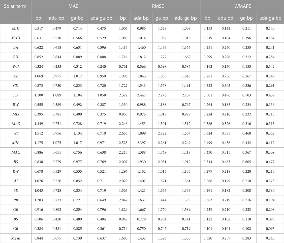
TABLE 4. MAE, RMSE, and WMAPE error results of the four models.

The combination of BP neural networks shows good optimization results, particularly the Adaboost-GA-BP model, which has the best overall optimization effect, especially during the summer and autumn seasons. This is because the Adaboost-GA-BP model effectively improves the defect of the steepest descent method easily falling into local optimal solutions, optimizes the network structure of the BP neural network, and it also has the characteristic of multiset optimization. In addition, the model has stronger nonlinear mapping ability and higher prediction accuracy.

The MAE error situation of the Adaboost-GA-BP model optimization is shown in Figure 11A with the circle representing the MAE error, which is located at the innermost part of the radial chart, indicating the best predictive performance. Among them, the MAE error optimization for 15 solar terms reached more than 10%, and the errors reduced by Winter Solstice, Pure Brightness, Beginning of Winter, Major Snow, and Awakening of Insects were 53.03%, 49.43%, 48.30%, 46.69%, and 33.93%, respectively, which ranked among the top five optimized outcomes.

FIGURE 11

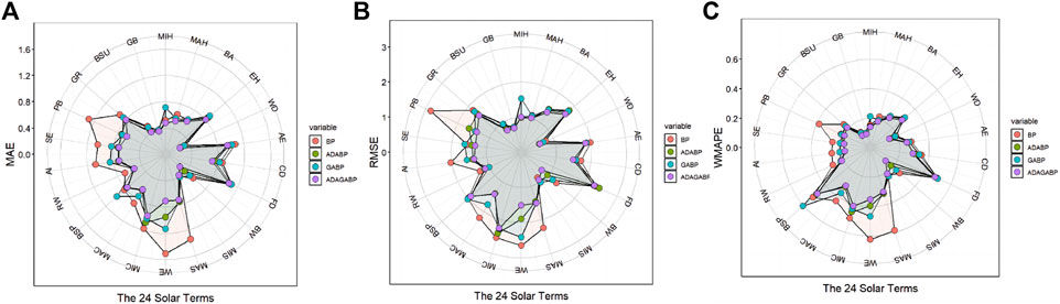
FIGURE 11. Comparison of MAE (A), RMSE (B) and WMAPE (C) results among BP (), Adaboost-BP (), GA-BP (), Adaboost-GA-BP () models.

The RMSE error optimization of the Adaboost-GA-BP model is shown in Figure 11B, with its circle located at the innermost part of the radar chart, indicating the best predictive performance. Thirteen solar terms achieved MAE error optimization of over 10%; among them, the errors reduced by Pure Brightness, Winter Equinox, Beginning of Winter, Major Cold and Awakening of Insects were 50.91%, 43.25%, 42.32%, 35.99% and 32.94%, respectively, ranking among the top five in terms of optimization effect.

The WMAPE error of the Adaboost-GA-BP model optimization is shown in the above Figure 11 with the circle representing the WMAPE error, which is located at the innermost part of the radial chart, indicating the best predictive performance. Among them, the WMAPE error optimization for 15 solar terms achieved a reduction of more than 10%, and the errors reduced by Pure Brightness, Beginning of Winter, Major Snow, Winter Solstice, and Awakening of Insects were 49.41%, 48.44%, 46.58%, 43.59%, and 34.12%, respectively, ranking among the top five in terms of optimization effectiveness.

In summary, the Adaboost-GA-BP model can effectively reduce errors and significantly improve the neural networks performance in processing data. By combining the 24 solar terms to partition the data, using the Adaboost-GA-BP model to predict PV power generation can result in more accurate predictions and promote the safety and stability of the power grid.

7 Discussion

By analyzing the photovoltaic power and meteorological data of three stations in Hebei Province, China, this article proposes an Adaboost-GA-BP model for short-term forecasting of photovoltaic power based on the characteristics of the 24 traditional solar terms in China. The conclusions are as follows:

• Introducing the 24 solar terms as a basis for data division in the modeling process can effectively extract meteorological data features o and improve training set similarity. Compared with dividing the data by half a month according to the Gregorian calendar, the division based on the 24 solar terms can reduce the average MAE, MSE, RMSE, and WMAPE by 15.68%, 40.57%, 14.68%, and 14.64%, respectively;

• Using the Ada-GA-BP model for short-term forecasting of photovoltaic power can effectively improve prediction accuracy. The BP neural network itself has strong nonlinear mapping capability, while Ada and GA optimize the network structure and initial weight threshold assignment on the BP neural network, respectively. Compared with BP, GA-BP and Adaboost-GA-BP, MAE, RMSE and WMAPE decreased by 23.42%, 18.12% and 22.28%, respectively. Adaboost-GA-BP has a strong advantage in processing multidimensional time series data with higher prediction accuracy.

• In the example model analysis in this paper, the prediction accuracy of short-term photovoltaic power is the highest when data are divided according to 24 solar terms and the Adaboost-GA-BP model is applied, indicating that the prediction scheme has a better fitting and prediction effect for the photovoltaic power data of Hebei Province, China.

• Through the empirical analysis of this paper, we draw the conclusion that using the 24 solar terms as the basis of data division can improve the internal similarity of data and help to improve the prediction effect of the model; And the ADABOOST-GA-BP model has the best prediction effect in short-term PV power prediction. It is of great significance to further regulate the operation of the power system and ensure its efficient and safe operation. Moreover, the research results of this paper also point out that improving the prediction accuracy can not only start from changing and optimizing the model, but also expand the analysis of the data, focusing on optimizing the way of data partitioning.

The limitations of this study include that the proposed data division method is based on data from Hebei, China, and its generalizability requires further exploration. The model is suitable for short-term photovoltaic power generation forecasting, but its efficiency for medium to long-term forecasting needs further optimization.

The data division and prediction models proposed in this paper can also be applied to load, wind power prediction and other fields. Due to the vast territory of China and its diverse and complex geographical and climatic features, if one wishes to utilize this dataset and model for analyzing data in southern China, it is essential to conduct localized analyses based on the specific locations of photovoltaic power stations. This is necessary to ensure the accuracy of the results for each data group. In future studies, it can be extended to other regions in the northern mid-latitudes, and the factors of the power-generated machine itself can be considered to further optimize the performance of the neural network and the model prediction accuracy.

Data availability statement

The original contributions presented in the study are included in the article/Supplementary material, further inquiries can be directed to the corresponding author.

Author contributions

YL, SD, and XH contributed to conception, methodology and design of the study. YL, SD, and XH performed the statistical analysis. YL, SD, and XH wrote the first draft of the manuscript. YL, SD, and XH wrote sections of the manuscript. HW was in charge of project management. All authors contributed to the article and approved the submitted version.

Funding

This work was supported by the National Natural Science Foundation of China (No. 41773092) and College Student Research and Career-creation Program of Beijing (No. S202210022136).

Conflict of interest

The authors declare that the research was conducted in the absence of any commercial or financial relationships that could be construed as a potential conflict of interest.

Publisher’s note

All claims expressed in this article are solely those of the authors and do not necessarily represent those of their affiliated organizations, or those of the publisher, the editors and the reviewers. Any product that may be evaluated in this article, or claim that may be made by its manufacturer, is not guaranteed or endorsed by the publisher.

References

Bacher, P., Madsen, H., and Nielsen, H. A. (2009). Online short-term solar power forecasting. Sol. Energy 83, 1772–1783. doi:10.1016/j.solener.2009.05.016

CrossRef Full Text | Google Scholar

Chen, C., Duan, S., Cai, T., and Dai, Q. (2011). Short-term prediction system for photovoltaic power generation based on fuzzy identification. Trans. China Electrotech. Soc. 26, 83–89.

Google Scholar

Chen, J., Wang, B., Lu, Z., and Shen, W. (2017). “Photovoltaic power generation prediction based on MEA-BP neural network,” in 2017 32nd Youth Academic Annual Conference of Chinese Association of Automation (YAC), Hefei, China, 19-21 May 2017 (IEEE), 387–392.

Google Scholar

Cheng, H., Cao, W., and Ge, P. (2012). “Forecasting research of long-term solar irradiance and output power for photovoltaic generation system,” in 2012 Fourth International Conference on Computational and Information Sciences, Chongqing, China, 17-19 August 2012 (IEEE), 1224–1227.

CrossRef Full Text | Google Scholar

Dai, Q., Duan, S., Cai, T., Chen, C., Chen, Z., and Qiu, C. (2011). Short-term irradiance-free power generation prediction model for photovoltaic systems based on weather type clustering identification. Proc. CSEE 31, 28–35.

Google Scholar

Das, U. K., Tey, K. S., Seyedmahmoudian, M., Mekhilef, S., Idris, M. Y. I., Horan, B., et al. (2018). Forecasting of photovoltaic power generation and model optimization: a review. Renew. Sustain. Energy Rev. 81, 912–928. doi:10.1016/j.rser.2017.08.017

CrossRef Full Text | Google Scholar

Deng, R., and Fang, Z. (2019). Yield analysis of financial products based on Spearman correlation analysis. Stat. Control 35, 164–167.

Google Scholar

Dolara, A., Leva, S., and Manzolini, G. (2015). Comparison of different physical models for PV power output prediction. Sol. Energy 119, 83–99. doi:10.1016/j.solener.2015.06.017

CrossRef Full Text | Google Scholar

Dong, C., Wang, Z., Bai, J., Jiang, J., Wang, B., and Liu, G. (2023). Review of ultra-short-term prediction methods for photovoltaic power generation. High. Volt. Technol.

Google Scholar

Fu, H., and Zhao, H. (2010). MATLAB neural network application design. 1. Beijing, China: China Machine Press, 89.

Google Scholar

Han, S., Zhang, L., Liu, Y., Ma, Y., Yan, J., and Li, L. (2020). A data sample division method for wind power prediction based on China's 24 solar terms. Int. Trans. Electr. Energy 30, e12342. doi:10.1002/2050-7038.12342

CrossRef Full Text | Google Scholar

Huang, L. (2008). BP neural network algorithm improvementand application research. Master Thesis. Chongqing, China: Chongqing Normal University.

Google Scholar

Huang, Y., Chen, S., Tan, X., Hu, M., and Zhang, C. (2022). “Power prediction method of distributed photovoltaic digital twin system based on GA-BP,” in 2022 4th International Conference on Electrical Engineering and Control Technologies (CEECT), Shanghai, China, 16-18 December 2022 (IEEE), 241–245.

CrossRef Full Text | Google Scholar

Huang, Y. (2021). Mid-term prediction of photovoltaic power based on long and short-term memory network. Master Thesis. Henan, China: North China University of Water Resources and Electric Power.

Google Scholar

Jiang, F., Wang, Z., and Zhang, P. (2019). Prediction of photovoltaic power generation based on gray-weighted Markov chain. Power Syst. Prot. Control 47, 55–60.

Google Scholar

Kar, T., and Melody, Y. (1992). Managerial applications of neural networks: the case of bank failure predictions. Manage. Sci. 38, 926–947. doi:10.1287/mnsc.38.7.926

CrossRef Full Text | Google Scholar

Lauret, P., Diagne, M., and David, M. (2014). A neural network post-processing approach to improving NWP solar radiation forecasts. Energy Procedia 57, 1044–1052. doi:10.1016/j.egypro.2014.10.089

CrossRef Full Text | Google Scholar

Li, C., Li, X., Zhao, R., Li, J., and Liu, X. (2008). Similar day selection algorithm for short-term load forecasting of electricity. Autom. Electr. Power Syst. 391, 69–73.

Google Scholar

Li, L., Liu, Z., Tseng, M., Zheng, S., and Lim, M. (2021). Improved tunicate swarm algorithm: solving the dynamic economic emission dispatch problems. Appl. Soft Comput. 108 (1), 107504. doi:10.1016/j.asoc.2021.107504

CrossRef Full Text | Google Scholar

Li, Y., He, Y., Su, Y., and Shu, L. (2016). Forecasting the daily power output of a gridconnected photovoltaic system based on multivariate adaptive regression splines. Appl. Energy 180, 392–401. doi:10.1016/j.apenergy.2016.07.052

CrossRef Full Text | Google Scholar

Liu, C., and Huang, Y. (2022). “Short term photovoltaic power prediction based on BP neural network optimized by improved sparrow search algorithm,” in 2022 4th International Academic Exchange Conference on Science and Technology Innovation (IAECST), Guangzhou, China, 09-11 December 2022 (IEEE), 314–317.

CrossRef Full Text | Google Scholar

Liu, X. (2017). The Formation of the twenty-four solar terms. Cult. Herit. 47, 1–7+157.

Google Scholar

Liu, Z., Li, L., Liu, Y., Liu, J., Li, H., and Shen, Q. (2021). Dynamic economic emission dispatch considering renewable energy generation: a novel multi-objective optimization approach. Energy 235, 121407. doi:10.1016/j.energy.2021.121407

CrossRef Full Text | Google Scholar

Lorenz, E., Scheidsteger, T., Hurka, J., Heinemann, D., and Kurz, C. (2011). Regional PV power prediction for improved grid integration. Prog. Photovolt. 19, 757–771. doi:10.1002/pip.1033

CrossRef Full Text | Google Scholar

Mandal, P., Madhira, S. T. S., Haque, A. U., Meng, J., and Pineda, R. L. (2012). Forecasting power output of solar photovoltaic system using wavelet transform and artificial intelligence techniques. Procedia Comput. Sci. 12, 332–337. doi:10.1016/j.procs.2012.09.080

CrossRef Full Text | Google Scholar

Meng, X., Xu, A., Zhao, W., Wang, H., Li, C., and Wang, H. (2018). “A new PV generation power prediction model based on GA-BP neural network with artificial classification of history day,” in 2018 International Conference on Power System Technology, Guangzhou, China, 06-08 November 2018 (IEEE), 1012–1017.

CrossRef Full Text | Google Scholar

Raza, M. Q., Nadarajah, M., and Ekanayake, C. (2016). On recent advances in PV output power forecast. Sol. Energy 136, 125–144. doi:10.1016/j.solener.2016.06.073

CrossRef Full Text | Google Scholar

Reikard, G. (2009). Predicting solar radiation at high resolutions: a comparison of time series forecasts. Sol. Energy 83, 342–349. doi:10.1016/j.solener.2008.08.007

CrossRef Full Text | Google Scholar

Sampson, J. R. (1976). Adaptation in natural and artificial systems. USA, Philadelphia, PA: SIAM.

Google Scholar

Schmelas, M., Feldmann, T., da-Costa-Fernandes, J., and Bollin, E. (2015). Photovoltaics energy prediction under complex conditions for a predictive energy management system. J. Sol. Energy. Eng. 137, 1–10. doi:10.1115/1.4029378

CrossRef Full Text | Google Scholar

Shi, S., and Li, J. (2016). PV power prediction based on particle swarm optimization LS-SVM. Hubei Electr. Power 40, 58–61.

Google Scholar

Sobri, S., Koohi-Kamali, S., and Abd. Rahim, N. (2018). Solar photovoltaic generation forecasting methods: a review. Energy Convers. Manag. 156, 459–497. doi:10.1016/j.enconman.2017.11.019

CrossRef Full Text | Google Scholar

Sui, B., and Zhang, J. (2020). The twenty-four solar terms: connotation, value, transmission and development. Agric. Hist. China 39, 111–117.

Google Scholar

Sun, J. (2019). Research on ultra-short-term power prediction of photovoltaic power generation Master. Wuhan, China: Wuhan University Of Technology.

Google Scholar

Tian, H., and Mao, Z. (2009). An ensemble ELM based on modified AdaBoost.RT algorithm for predicting the temperature of molten steel in ladle furnace. IEEE Trans. Autom. Sci. Eng. 7, 73–80.

Google Scholar

Wang, F., Xuan, Z., Zhen, Z., Li, K., Wang, T., and Shi, M. (2020). A day-ahead PV power forecasting method based on LSTM-RNN model and time correlation modification under partial daily pattern prediction framework. Energy Convers. Manag. 212, 112766. doi:10.1016/j.enconman.2020.112766

CrossRef Full Text | Google Scholar

Wang, H., Yi, H., Peng, J., Wang, G., Liu, Y., Jiang, H., et al. (2017). Deterministic and probabilistic forecasting of photovoltaic power based on deep convolutional neural network. Energy Convers. Manag. 153, 409–422. doi:10.1016/j.enconman.2017.10.008

CrossRef Full Text | Google Scholar

Wang, L., Mao, M., Xie, J., Liao, Z., Zhang, H., and Li, H. (2023). Accurate solar PV power prediction interval method based on frequency-domain decomposition and LSTM model. Energy 262, 125592. doi:10.1016/j.energy.2022.125592

CrossRef Full Text | Google Scholar

Wang, X., and Chu, T. (2014). Non-parametric statistics. 2. Beijing, China: Tsinghua University Press, 182.

Google Scholar

Xie, J., and Hong, T. (2018). Load forecasting using 24 solar terms. J. Mod. Power Syst. Cle. 6, 208–214. doi:10.1007/s40565-017-0374-0

CrossRef Full Text | Google Scholar

Yang, H., Huang, C., Huang, Y., and Pai, Y. (2014). A weather-based hybrid method for 1-day ahead hourly forecasting of PV power output. IEEE Trans. Sustain. Energy 5, 917–926. doi:10.1109/tste.2014.2313600

CrossRef Full Text | Google Scholar

Yang, X., Wang, S., Peng, Y., Chen, J., and Meng, L. (2023). Short-term photovoltaic power prediction with similar-day integrated by BP-AdaBoost based on the Grey-Markov model. Electr. Pow. Syst. Res. 215, 108966. doi:10.1016/j.epsr.2022.108966

CrossRef Full Text | Google Scholar

Yang, Z., Mourshed, M., Liu, K., Xu, X., and Feng, S. (2020). A novel competitive swarm optimized RBF neural network model for short-term solar power generation forecasting. Neurocomputing 397, 415–421. doi:10.1016/j.neucom.2019.09.110

CrossRef Full Text | Google Scholar

Yao, T., Wang, J., Wu, H., Zhang, P., Li, S., Wang, Y., et al. (2021b). A photovoltaic power output dataset: multi-source photovoltaic power output dataset with python toolkit. Sol. Energy 230, 122–130. doi:10.1016/j.solener.2021.09.050

CrossRef Full Text | Google Scholar

Yao, T., Wang, J., Wu, H., Zhang, P., Li, S., Wang, Y., et al. (2021a). Pvod v1.0: A photovoltaic power output dataset 2021. Science Data Bank.

Google Scholar

Zhang, C., and Zhang, M. (2022). Wavelet-based neural network with genetic algorithm optimization for generation prediction of PV plants. Energy Rep. 8, 10976–10990. doi:10.1016/j.egyr.2022.08.176

CrossRef Full Text | Google Scholar

Zhou, T., Li, X., and Wang, P. (2021). Statistics and practice on the trend’s reversal and turning points of Chinese stock indices based on gann’s time theory and solar terms effect. Mathematics 9, 1713. doi:10.3390/math9151713

CrossRef Full Text | Google Scholar