Flexibility-expansion planning of multi-energy systems by energy storage for participating in balancing-power markets

The growing need for balancing power combined with the shutdown of conventional power plants requires new balancing-power providers. In this context, industrial energy systems are particularly promising. However, the main task of industrial energy systems is to provide various energy forms. For this purpose, they operate interconnected units to maximize efficiency, but the interconnected operation also increases complexity, limiting flexibility due to the need to supply fixed demands. Energy storage can increase the flexibility of current and future industrial energy systems, thus enhancing the potential for sector coupling within the overall energy system at a low cost. To improve the flexibility of industrial energy systems, we propose a design optimization framework that accounts for investment in energy storage and for the provision of balancing power. Since the request of balancing power is uncertain, we present a stochastic program for the balancing-power market and propose two ways to model storage that both derive feasible storage operations while being computationally efficient. In a case study of a multi-energy system, cost savings between 6% and 17% can be achieved by increasing flexibility for participation in the balancing-power market with investment in heat storage. The sensitivity analysis identifies heat storage as particularly advantageous for heat-driven energy systems. Our method combines long-term investment decisions with short-term operational uncertainties to identify optimal investment decisions, which enhance the energy system’s flexibility for the provision of balancing power.

1 Introduction

Renewable energies have become a major energy source globally in recent years (IEA, 2021). However, energy supply by renewable energies depends on weather conditions and seasons. The resulting variability renders balancing supply and demand in the electricity grid increasingly challenging (Brouwer et al., 2014).

Short-term imbalances between supply and demand are settled by balancing power. Balancing power is an ancillary service offered by electricity providers or consumers to support grid stability: positive balancing power is provided by increasing supply or decreasing demand; negative balancing power works vice versa (Ocker and Ehrhart, 2017).

Traditionally, balancing power is mainly supplied by conventional power plants (Rancilio et al., 2022). Due to political, environmental, and economic reasons, these power plants are increasingly shut down and, therefore, no longer provide balancing power. Thus, new balancing-power providers are needed. For this purpose, multi-energy systems that supply industrial sites are particularly suited since they handle large amounts of energy and power.

These multi-energy systems are complex as they commonly produce several energy forms (e.g., heat, cooling, and electricity) by operating a set of interconnected units (Bischi et al., 2014). This complexity limits the flexibility required for the provision of balancing power since the energy demands need to be supplied at all times and are not flexible in general. In this case, flexibility has to be found within the multi-energy system. One solution to enhance flexibility is energy storage to decouple heat supply and demand (Guelpa et al., 2019). Therein, energy storage has been recently discussed for the flexibilization of industrial energy systems (Prenzel et al., 2023). Here, energy storage can already provide flexibility in the short term without changing the entire industrial energy system. Employing sector coupling can make these storage solutions an essential first step toward reducing carbon emissions in energy-intensive industries (Baumgärtner et al., 2019b) while being less costly than batteries. In the long term, storage supports the flexibility of industrial energy systems that are either electrified or operated using green fuels. Therefore, the storage can remain valuable in low-carbon multi-energy systems.

In recent years, participation in balancing-power markets has been extensively studied for industrial applications. The studies reveal significant operational savings in terms of costs, e.g., for an air separation unit with cryogenic energy storage (Zhang et al., 2015), for a combined heat-and-power plant with heat storage (Kumbartzky et al., 2017), for a batch production system with a utility system (Leenders et al., 2020), for combined cycles (Zhang et al., 2023), for electrified district-heating networks (Javanshir et al., 2023), and for energy-intense processes, such as an aluminum mill (Schäfer et al., 2019; Varelmann et al., 2022), a cement plant (Bohlayer et al., 2020), and a chlor-alkali process (Lahrsen et al., 2022).

Since the request of balancing power is uncertain, the balancing-power market model needs to consider uncertainty. For this purpose, the cited studies mainly use stochastic programming (Birge and Louveaux, 2011). In the stochastic program, market participation and system operation are commonly modeled in several stages. The resulting optimization problems, however, tend to be difficult to solve, resulting in prohibitive solution times. Thus, solving these problems commonly requires specialized solution techniques, such as Benders decomposition (Varelmann et al., 2022) or customized approaches (Schäfer et al., 2019).

The complexity of energy system optimization increases further when design decisions are included since design decisions couple all the time steps within the operation. For multi-energy systems, the design optimization is proven to be strongly NP-hard (Goderbauer et al., 2019) even without considering balancing power. Early approaches to considering balancing power during design, therefore, avoid solving this decision-making problem within a single optimization problem. In contrast, the operation and investment decisions are evaluated in two consecutive steps: the participation in the balancing-power market is studied as operational optimization (Muche et al., 2016) or in market simulations (Angenendt et al., 2020; Schlachter et al., 2020). Therein, the investment decision is analyzed through a sensitivity analysis concerning component sizing, storage properties, and investment cost. However, this consecutive approach may lead to suboptimal investment decisions, such as to storage systems that are too small. However, providing flexibility requires oversizing (Schäfer et al., 2020), making optimal investment decisions necessary.

Thus, investment decisions in storage units lead to a complex decision-making problem if the balancing-power market is included in design optimization. The consequence of providing balancing power is uncertainty within the energy system operation since the request for balancing power is uncertain. In contrast, price uncertainties in electricity and gas markets influence the system costs but not necessarily the operation. Thus, uncertainties from the balancing-power market should be considered in design optimization to ensure a feasible operation in case of request. Recent approaches integrate uncertainties into the design optimization, such as short-term operational uncertainties (Mavromatidis et al., 2018; Teichgraeber and Brandt, 2020), long-term trends (Hoettecke et al., 2022), and transition pathways (Bohlayer et al., 2021). In this context, Roh et al. (2019), Teichgraeber and Brandt (2020), and Schäfer et al. (2020) highlight the possible benefits of including the provision of ancillary services in design optimization. Therefore, a recent approach by Srinivasan et al. (2023) integrates the provision of balancing-power capacity in the design optimization of multi-energy systems. However, the request of balancing power and its associated revenues are not considered within the design optimization model.

Here, we fill this gap and include the provision of balancing power in the design optimization for multi-energy systems. Therefore, the design optimization considers the energy system’s flexibility by explicitly modeling the request of balancing power. The proposed design optimization model combines long-term investment decisions with short-term uncertainties of participation in the balancing-power market. The study aims to establish a model that is computationally tractable for practical applications. Thus, we introduce a simplified model of the balancing-power market. This model is a two-stage stochastic program that considers the most important market features and uncertainties. However, the time-coupling of the storage unit makes the optimization intractable. We, therefore, propose two storage formulations, namely, same and flexible, that both derive feasible storage operations while being computationally efficient.

The proposed method of flexibility-expansion planning helps identify trade-offs between the energy system design and flexible operation in balancing-power markets. While the method is generally applicable to energy storage, our focus is on heat storage as a promising technology for the flexibilization of multi-energy systems.

The proposed method extends on our previous conference contribution (Nolzen et al., 2021). Here, the method is adapted and presented in more detail, followed by a detailed analysis of heat storage as an option for increasing the flexibility of the multi-energy system. For this purpose, the method is adapted by disregarding the bidding problem, allowing for more efficient integration of the balancing-power market into the design optimization. Subsequently, we elaborate more on the case study to explore the benefits of heat storage for flexibilizing multi-energy systems.

The remainder of this paper is organized as follows: in Section 2, we propose a method to model the balancing-power market, including storage units, into a design optimization. In Section 3, our method is applied to a case study of a multi-energy system. Finally, Section 4 describes our conclusions.

2 Optimized storage investments in flexibility for balancing-power markets

The flexibility-expansion planning method is proposed for optimal investments in flexibility for balancing-power markets. The proposed method optimizes long-term investment decisions, considering the short-term flexibility required for the balancing-power market.

Balancing-power market participation introduces uncertainty to the optimization problem. The uncertainty is modeled with stochastic optimization. However, in stochastic optimization, the operation of storage units is challenging since their time-coupling causes the optimization problem to grow exponentially.

Thus, we propose two formulations to model storage: same and flexible. Both formulations avoid exponential growth of the optimization problem. The optimization problem still allows for the analysis of trade-offs between long-term investment decisions in storage and short-term operation to provide balancing power.

In Section 2.1, a stochastic program is introduced for balancing-power market participation. This approach considers a wide range of different market designs, including the most common European balancing-power markets. Section 2.2 introduces the general energy system model suitable for greenfield and brownfield optimization. Here, the model is presented for the retrofit with energy storage. Finally, Section 2.3 explains the modeling of energy storage units. We propose two formulations, namely, same and flexible for storage units that determine the economic benefits of investments in storage units toward the energy system’s flexibility.

2.1 Balancing-power market participation as a two-stage stochastic program

Balancing power compensates for imbalances between electricity supply and demand in the electricity grid. Usually, transmission system operators deploy balancing power via the balancing-power market. In the balancing-power market, participating energy systems can offer positive and/or negative balancing power. Suppose the transmission system operator requests positive balancing power; energy systems increase the amount of electricity fed into the electricity grid or reduce the amount of electricity drawn from the electricity grid. Inversely, if the transmission system operator requests negative balancing power, energy systems decrease the amount of electricity fed into the electricity grid or increase the amount of electricity drawn from the electricity grid.

Commonly, energy systems receive two types of payments for the provision of balancing power: the capacity price $p_t^{\text{cp,}+\text{/}-}$ (in €/MW) is paid for the provision of balancing-power capacity; the energy price $p_t^{\text{ep,}+\text{/}-}$ (in €/MWh) compensates the requested amount of balancing energy. Both prices are specific for positive and negative balancing power. Thus, four prices are tendered at the balancing-power market.

Participation in the balancing-power market introduces uncertainty to the energy system operation due to the uncertain request of balancing power. To cover this uncertainty, we model the participation in the balancing-power market as a two-stage stochastic program following Leenders et al. (2020).

Figure 1 illustrates the two-stage stochastic program, including the decisions taken at both stages. The first stage of the stochastic program models the tender at the balancing-power market. The tender consists of the amount of positive $B{P}_t^{+}$ and negative balancing power $B{P}_t^{-}$, the capacity prices $p_t^{\text{cp,}+\text{/}-}$, and the energy prices $p_t^{\text{ep,}+\text{/}-}$. The second stage of the stochastic program models the scenario-dependent operation of the energy system. Due to the uncertain request of balancing power, the second stage considers three request scenarios ω ∈ Ω = {none, pos, neg} for the operation of the energy system in each time step t ∈ T: no request of balancing power (none), the request of positive balancing power (pos), and the request of negative balancing power (neg). The three request scenarios are assigned scenario probabilities π_t,ω that sum up to 1.

FIGURE 1

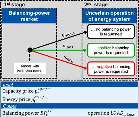
FIGURE 1. The two-stage stochastic program considers the balancing-power market participation, in the first stage, including the most important market features such as capacity prices, energy prices, and the actual offer of balancing power. In the second stage, balancing-power provision is modeled as three request scenarios, ω ∈ Ω per time step t ∈ T, that consider the operation of the energy system.

The method optimizes design decisions considering the balancing-power market. Therefore, the design optimization requires a sufficient approximation of the revenues in the balancing-power market. For optimal investment decisions, the stochastic program does not explicitly consider the pricing mechanism of the balancing-power market, such as marginal pricing or pay-as-bid pricing (Rancilio et al., 2022). As a result, the acceptance and the request for balancing power take place at fixed pre-defined prices, which are not optimized in the stochastic program within the design optimization. However, once the design is determined, an operational optimization with optimized bidding may increase revenues (Bohlayer et al., 2020) but, at the same time, would require reliable and accurate price predictions (Bringedal et al., 2021). For long-term investment decisions, these price predictions are typically unavailable.

Thus, we neglect optimized bidding and assume price levels such that the tenders are always accepted in the market. The presented stochastic program accounts for the operational uncertainty introduced by the balancing-power market participation. Therefore, balancing-power market participation is remunerated with capacity prices for the provision of balancing power and energy prices for the request of balancing power. Our modeling approach can be used for balancing-power market designs with both marginal pricing and pay-as-bid pricing.

2.2 Retrofit optimization of energy systems with balancing-power market participation

Here, we introduce the optimization model of the energy system. The presented model focuses on retrofitting with energy storage. However, the model is also suitable for greenfield optimization with further components. The optimization model considers long-term investment decisions for the energy system’s design and short-term operational decisions associated with participation in the balancing-power market and energy system’s operation. The considered energy system model represents a typical industrial energy system that supplies industrial energy demands for various products p ∈ P, such as electricity, heat, and cooling, at time steps t ∈ T.

The objective function is presented in Section 2.2.1, including all necessary economic constraints for participation in the balancing-power market. Subsequently, the general product balance (Section 2.2.2) and electricity balance adapted to the balancing-power market (Section 2.2.3) are introduced. The constraints for the operation of the underlying energy systems are presented in Supplementary Appendix S1.

2.2.1 Objective function and market participation

The objective function minimizes the total annualized cost TAC as follows:

$\min TAC=CAPEX+OPEX.(1)$

The total annualized cost TAC consists of costs for annualized capital expenditure CAPEX and the yearly operational cost OPEX.

The annualized capital expenditure CAPEX arises from the investment decision in a storage unit for a product p (e.g., electricity and heat) as

$CAPEX=\sum _{p\in P}{C}_p^{\text{stor}}\cdot cos{t}_p^{\text{inv}}.(2)$

The capacity of a storage unit $C_p^{\text{stor}}$ is multiplied by the annualized specific investment cost $cos{t}_p^{\text{inv}}$. In principle, investment in other technologies could be included. Here, we focus on energy storage since the resulting time-coupling requires a particular treatment.

The yearly operational cost

$OPEX=\sum _{t\in T}{\mathrm{\Delta }}_t\cdot \sum _{\omega \in \mathrm{\Omega }}{\pi }_{t,\omega }\cdot OPE{X}_{t,\omega }(3)$

sums up the scenario-based operational cost of all time steps and scenarios within a year. The OPEX takes into account the operation of the energy system, including the provision of balancing power. In Eq. 3, the scenario-based operational cost OPEX_t,ω is multiplied with the respective request probability π_t,ω to obtain the expected cost in each time step t ∈ T. Subsequently, the expected cost in each time step is multiplied by the weight of each time step Δ_t within an entire year since the optimization model considers typical periods (Baumgärtner et al., 2019a). Conceptually, the method does not require typical periods. However, the usage of typical periods is common in the design optimization of multi-energy systems since computation time can be saved with small losses in the solution quality (Hoffmann et al., 2020).

The scenario-based operational cost

$\begin{array}{c}OPE{X}_{t,\omega }=C_{t,\omega }^{\text{GAS}}+C_t^{\text{DAM}}-R_t^{\text{DAM}}-R_t^{\text{BPM,cp}}-R_{t,\omega }^{\text{BPM,ep}}\\ \forall t\in T,\omega \in \mathrm{\Omega }\end{array}(4)$

considers the costs and revenues for market participation and energy system operation. For each time step t ∈ T and scenario ω ∈ Ω, the scenario-based operational cost OPEX_t,ω comprises the costs for the purchase of gas $C_{t,\omega }^{\text{GAS}}$ and electricity $C_t^{\text{DAM}}$ at the day-ahead market, the revenues from the sale of electricity $R_t^{\text{DAM}}$ at the day-ahead market, the revenues for the provision of capacity $R_t^{\text{BPM,cp}}$ at the balancing-power market, and the actual delivery of balancing power $R_{t,\omega }^{\text{BPM,ep}}$.

The cost for gas $C_{t,\omega }^{\text{GAS}}$ is calculated from the consumed gas BUY_gas,t,ω and the gas price $p_t^{\text{gas,buy}}$:

$C_{t,\omega }^{\text{GAS}}=BU{Y}_{\text{gas},t,\omega }\cdot p_t^{\text{gas,buy}}\forall t\in T,\omega \in \mathrm{\Omega }.(5)$

Equations 6, 7 model the cost for the purchase and sale of electricity.

$R_t^{\text{DAM}}=SEL{L}_{\text{el},t}\cdot p_t^{\text{el,sell}}\forall t\in T,(6)$

$C_t^{\text{DAM}}=BU{Y}_{\text{el},t}\cdot p_t^{\text{el,buy}}\forall t\in T.(7)$

Equation 6 computes the revenues from the sale of electricity by multiplying the sold amount of electricity SELL_el,t with the electricity price $p_t^{\text{el,sell}}$. Similarly, Eq. 7 calculates the cost of purchasing electricity. Regardless of the request for balancing power, the same amount of electricity needs to be purchased or sold on the day-ahead market.

Note that the variables SELL_el,t and BUY_el,t are not dependent on the request scenario ω ∈ Ω for the purchase and sale of electricity. Thus, these variables are missing the index ω in contrast to the remaining variables for purchasing and selling products.

Equations 8, 9 consider the revenues for the provision of balancing power from the capacity price $p_t^{\text{cp,}+\text{/}-}$ and the energy price $p_t^{\text{ep,}+\text{/}-}$.

$R_t^{\text{BPM,cp}}=B{P}_t^{+}\cdot p_t^{\text{cp,}+}+B{P}_t^{-}\cdot p_t^{\text{cp,}-}\forall t\in T,(8)$

$R_{\omega ,t}^{\text{BPM,ep}}={\alpha }_{\omega }^{+}\cdot B{P}_t^{+}\cdot p_t^{\text{ep,}+}+{\alpha }_{\omega }^{-}\cdot B{P}_t^{-}\cdot p_t^{\text{ep,}-}\forall t\in T,\omega \in \mathrm{\Omega }.(9)$

Equation 8 computes the provision of capacity for positive balancing power $B{P}_t^{+}$ and negative balancing power $B{P}_t^{-}$. Therein, the provision of capacity is remunerated with the capacity price $p_t^{\text{cp,}+\text{/}-}$, thus assuming that tenders in the balancing-power market are always accepted with the deterministic capacity price. As discussed in Section 2.1, the idea is to approximate the revenues in the balancing-power market sufficiently. Therefore, this modeling approach assumes the selection of pre-defined capacity prices that are sufficiently low to be accepted in the balancing-power market. If relatively high capacity prices are chosen for the optimization, the acceptance probability decreases such that acceptance and rejection need to be considered in the model.

In Eq. 9, the energy price $p_t^{\text{ep,}+\text{/}-}$ remunerates the request of positive and negative balancing power. Since the request is only compensated in the respective request scenario, we introduce the binary parameters ${\alpha }_{\omega }^{+}$ and ${\alpha }_{\omega }^{-}$. The binary parameters ${\alpha }_{\omega }^{+}$ and ${\alpha }_{\omega }^{-}$ model the scenario-dependent remuneration and are set to 1 if balancing power is requested and 0 otherwise. Therefore, ${\alpha }_{\omega }^{+/-}$ has different values for the three request scenarios described in Section 2.1: both parameters ${\alpha }_{\omega }^{+}$ and ${\alpha }_{\omega }^{-}$ are 0 if no balancing power is offered (ω = none); ${\alpha }_{\omega }^{+}$ is set to 1 for the scenario in which positive balancing power is supplied (ω = pos); and ${\alpha }_{\omega }^{-}$ is set to 1 for the scenario in which negative balancing power is supplied (ω = neg).

Commonly, balancing power is offered in time slices, e.g., each time slice is 4 hours for the German market. However, the temporal resolution within the optimization model is usually higher than the length of the time slices, e.g., 1 hour. That means a time slice comprises N time steps. Following this, Eqs 10, 11 ensure that the same amount of positive and negative balancing power is offered within each time slice:

${BP}_t^{+}={BP}_{t+a}^{+}\forall t\in T:\left(t-1\right)\mid N=0,a\in \left\{\mathrm{1,2},\dots ,N-1\right\},(10)$

${BP}_t^{-}={BP}_{t+a}^{-}\forall t\in T:\left(t-1\right)\mid N=0,a\in \left\{\mathrm{1,2},\dots ,N-1\right\}.(11)$

The time steps are represented by integers starting from 1, 2 … T. Thus, time step t indicates the beginning of a new time slice if t − 1 is divisible by N with no remainder. Subsequently, the amount of positive balancing power (Eq. 10) and negative balancing power (Eq. 11) that the energy system can supply is the same in the next N time steps.

2.2.2 General product balance

The energy system supplies or demands products p ∈ P, e.g., heat or natural gas. Due to the provision of balancing power, the electricity balance is adjusted and presented separately in Section 2.2.3. Thus, the general product balance is formulated for all products except for electricity p ∈ P $\backslash \left\{\mathrm{e}\mathrm{l}\right\}$, time steps t ∈ T, and request scenarios ω ∈ Ω:

$\begin{array}{c}de{m}_{p,t}=\sum _{u\in U}{P}_{u,p,t,\omega }+BU{Y}_{p,t,\omega }+OU{T}_{p,t,\omega }^{\text{stor}}-I{N}_{p,t,\omega }^{\text{stor}}\\ \forall p\in P\backslash \left\{\mathrm{e}\mathrm{l}\right\},t\in T,\omega \in \mathrm{\Omega }.\end{array}(12)$

In Eq. 12, the product demand dem_p,t has to be fulfilled independently from the request scenario ω ∈ Ω. Therein, the product demand dem_p,t is covered by supply or additional demand of production units P_u,p,t,ω and by buying products BUY_p,t,ω. Here, P_u,p,t,ω is negative if the production unit u demands a product (e.g., natural gas) and positive if the production unit u supplies a product (e.g., heat). In addition, charging $I{N}_{p,t,\omega }^{\text{stor}}$ or discharging $OU{T}_{p,t,\omega }^{\text{stor}}$ of the storage unit for product p adjusts the product balance.

Note that commonly, certain products, e.g., heat, cannot be purchased. In this case, the variable BUY_p,t,ω is set to 0. As a result, only storage and production units cover the demand dem_p,t for such a product p.

2.2.3 Electricity balance including balancing-power provision

The electricity balance differs from the general product balance since the electricity balance considers the possibility to exchange electricity with the grid via the day-ahead market and the balancing-power market. For each time step t ∈ T and scenario ω ∈ Ω, the electricity balance thus results in

$\begin{array}{ll}\hfill & \sum _{u\in U}{P}_{u,\mathrm{e}\mathrm{l},t,\omega }+BU{Y}_{\text{el},t}+{\alpha }_{\omega }^{-}\cdot B{P}_t^{-}+OU{T}_{\text{el},t,\omega }^{\text{stor}}-I{N}_{\text{el},t,\omega }^{\text{stor}}\hfill \\ \hfill & =de{m}_{\text{el},t}+{\alpha }_{\omega }^{+}\cdot B{P}_t^{+}+SEL{L}_{\text{el},t}\forall t\in T,\omega \in \mathrm{\Omega }.\hfill \end{array}(13)$

The electricity demand dem_el,t is satisfied by the sum of the energy system’s electricity production P_u,el,t,ω as well as the sale SELL_el,t or purchase BUY_el,t of electricity on the day-ahead market. If available, battery storage can be used to cover the electricity balance by charging $I{N}_{\text{el},t,\omega }^{\text{stor}}$ or discharging $OU{T}_{\text{el},t,\omega }^{\text{stor}}$.

Equation 13 also considers the provision of positive $B{P}_t^{+}$ and negative balancing power $B{P}_t^{-}$ by the binary parameters ${\alpha }_{\omega }^{+}$ and ${\alpha }_{\omega }^{-}$. The binary parameters ${\alpha }_{\omega }^{+}$ and ${\alpha }_{\omega }^{-}$ take values of 0 or 1 depending on the request of balancing power.

Overall, the demands of the industrial energy system are pre-defined and deterministic, i.e., within each time step t ∈ T, the demands are the same for each request scenario ω ∈ Ω. Therefore, these pre-defined demands must be covered independently from the provision of balancing power. Thus, the flexibility for the provision of balancing power is realized by adjusting the operation of the industrial energy system by either switching between production units (e.g., from combined heat-and-power units to boilers) or by using storage.

2.3 Modeling of storage units in the balancing-power market

Storage units store products in a certain time step and withdraw the products at a later time step. In contrast to quasi-steady state formulations of energy conversion technologies, storage models introduce state variables at the storage level (Sass and Mitsos, 2019). Thus, the time-coupling of all time steps resulting from the investment decision additionally leads to a time-coupling at the operational level, as the state variables introduce a temporal path dependency. Since storage units couple the time steps t ∈ T in an optimization problem, modeling storage units substantially increases complexity within the stochastic program described in Section 2.1.

Due to the three request scenarios ω ∈ Ω, our problem yields three possible operations of the storage unit for each time step t ∈ T. Thus, the number of possible storage levels increases with 3^|T|, and the problem gets computationally intractable with only a few time steps.

Hence, we present two formulations to restrict the possible storage level in each time step. Figure 2 provides an overview of the two proposed formulations: same and flexible. The storage formulation same considers the same storage level across all request scenarios regardless of the request for balancing power. In contrast, the storage formulation flexible considers the lowest storage level across all request scenarios for the next time step. Both formulations same and flexible pass only one distinct storage level to the next time step. Therefore, the problems remain computationally tractable since the number of scenarios increases with 3 ⋅|T| instead of 3^|T|. However, both proposed storage formulations restrict recourse in the optimization problem, i.e., the information that is passed to the next time step is restricted.

FIGURE 2

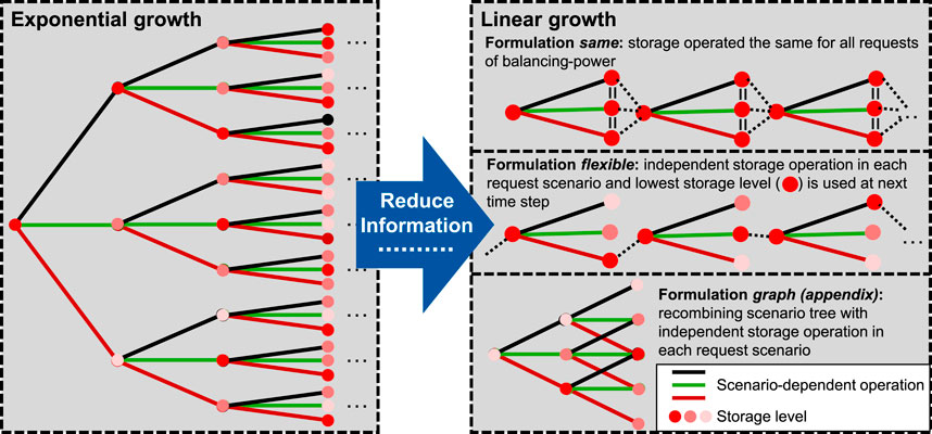
FIGURE 2. Modeling the participation in the balancing-power market leads to an exponential growth of the scenarios (left). To keep the problem tractable, we restrict the information, i.e., storage level, passed to the next time step. For all three proposed scenarios, same, flexible, and graph (right), the number of scenarios increases linearly.

As a further idea, we present the storage formulation graph based on a recombining trinomial tree in Supplementary Appendix S2. The recombining trinomial tree allows for recourse and uses the advantage of recombination: the number of possible storage levels still grows linearly with 3 ⋅|T|. However, compared to our other approaches, the model is computationally expensive, while extensive preliminary studies have shown only a small benefit (cf. Supplementary Appendix S2). Thus, the approach is not pursued any further.

Both formulations same and flexible ensure a feasible operation since the storage level is always at a sufficient level. In this context, sufficient means that the energy stored in the storage unit is available and ready for use when required for the energy system’s operation, even under a potential request of balancing power. Therefore, both formulations allow us to assess the economic benefit that storage provides for the flexibilization of the energy system.

In Section 2.3.1, we present general modeling equations to model storage units. Subsequently, we present the additional equations for formulation same in Section 2.3.2 and formulation flexible in Section 2.3.3.

2.3.1 General storage equations

This section presents the general storage equations Eqs 14–22 that are used both in formulation same and formulation flexible. The general formulation can be used for storing an arbitrary product p.

In case an investment is made in the storage unit, Eqs 14, 15 model the capacity limits as

$C_p^{\text{stor}}\le ca{p}_p^{\text{stor,max}}\cdot {\gamma }_p^{\text{stor}}\forall p\in P,(14)$

$C_p^{\text{stor}}\ge ca{p}_p^{\text{stor,min}}\cdot {\gamma }_p^{\text{stor}}\forall p\in P.(15)$

The binary variable ${\gamma }_p^{\text{stor}}$ equals one if an investment in a storage unit for product p is made. In this case, the newly installed storage capacity $C_p^{\text{stor}}$ is restricted between minimum $ca{p}_p^{\text{stor,min}}$ and maximum potential storage capacity $ca{p}_p^{\text{stor,max}}$.

Since the newly installed storage unit is used in all time steps t ∈ T, the variable $C_p^{\text{stor}}$ couples all time steps within the optimization problem. Subsequently, Eq. 16 ensures that the storage level is always greater than 0 and limits the storage level $ST{L}_{p,t,\omega }^{\text{stor}}$ to the installed storage capacity $C_p^{\text{stor}}$:

$0\le ST{L}_{p,t,\omega }^{\text{stor}}\le C_p^{\text{stor}}\forall p\in P,t\in T,\omega \in \mathrm{\Omega }.(16)$

Similar to Baumgärtner et al. (2019b), we assume a limit of the storage power for charging $I{N}_{p,t,\omega }^{\text{stor}}$ and discharging $OU{T}_{p,t,\omega }^{\text{stor}}$ as a fixed fraction of the storage capacity by the factor $pc{r}_p^{\text{stor}}$ that is multiplied by the storage capacity $C_p^{\text{stor}}$:

$OU{T}_{p,t,\omega }^{\text{stor}}\le pc{r}_p^{\text{stor}}\cdot C_p^{\text{stor}}\forall p\in P,t\in T,\omega \in \mathrm{\Omega },(17)$

$I{N}_{p,t,\omega }^{\text{stor}}\le pc{r}_p^{\text{stor}}\cdot C_p^{\text{stor}}\forall p\in P,t\in T,\omega \in \mathrm{\Omega }.(18)$

Thus, Eqs 17, 18 limit the amount of product p to discharge $OU{T}_{p,t,\omega }^{\text{stor}}$ and charge the storage unit $I{N}_{p,t,\omega }^{\text{stor}}$ depending on the storage capacity $C_p^{\text{stor}}$.

In each time step t ∈ T and scenario ω ∈ Ω, either charging or discharging of the storage unit is allowed. Equations 19–21 restricts the operation of the storage unit accordingly:

${ϵ}_{p,t,\omega }^{\text{stor,in}}+{ϵ}_{p,t,\omega }^{\text{stor,out}}\le 1\forall p\in P,t\in T,\omega \in \mathrm{\Omega },(19)$

$OU{T}_{p,t,\omega }^{\text{stor}}\le pc{r}_p^{\text{stor}}\cdot ca{p}_p^{\text{stor,max}}\cdot {ϵ}_{p,t,\omega }^{\text{stor,out}}\forall p\in P,t\in T,\omega \in \mathrm{\Omega },(20)$

$I{N}_{p,t,\omega }^{\text{stor}}\le pc{r}_p^{\text{stor}}\cdot ca{p}_p^{\text{stor,max}}\cdot {ϵ}_{p,t,\omega }^{\text{stor,in}}\forall p\in P,t\in T,\omega \in \mathrm{\Omega }.(21)$

The binary variables ${ϵ}_{p,t,\omega }^{\text{stor,in}}$ and ${ϵ}_{p,t,\omega }^{\text{stor,out}}$ indicate if the storage unit is charged or discharged in time step t ∈ T and scenario ω ∈ Ω. Equation 19 ensures that either ${ϵ}_{p,t,\omega }^{\text{stor,in}}$ or ${ϵ}_{p,t,\omega }^{\text{stor,out}}$ equal one in each time step and scenario to either allow charging or discharging. Subsequently, Eqs 20, 21 restrict either the maximum power for discharging $OU{T}_{p,t,\omega }^{\text{stor}}$ or charging $I{N}_{p,t,\omega }^{\text{stor}}$ the storage unit to 0 if one of the binary variables ${ϵ}_{p,t,\omega }^{\text{stor,in}}$ and ${ϵ}_{p,t,\omega }^{\text{stor,out}}$ equals 0. Overall, Eqs 17–21 constrain the storage operation: Eqs 17, 18 limit the maximum power of the storage; Eqs 19–21 restrict the charging and discharging per time step.

A key step to keep the optimization problem tractable is to reduce the information passed to the next time step. Here, the storage level needs to be passed on to the next time step. In principle, each scenario ω ∈ Ω = {none, pos, neg} could lead to a different storage level, and, thus, to 3^|T| storage levels. To avoid this growth of the scenario tree, we propose to forward only one storage level per time step. Equation 22 ensures the same storage levels for all scenarios ω ∈ Ω, in each time step t ∈ T, with a non-anticipativity constraint:

$ST{L}_{p,t,\mathrm{p}\mathrm{o}\mathrm{s}}^{\text{stor}}=ST{L}_{p,t,\mathrm{n}\mathrm{o}\mathrm{n}\mathrm{e}}^{\text{stor}}=ST{L}_{p,t,\mathrm{n}\mathrm{e}\mathrm{g}}^{\text{stor}}\forall p\in P,t\in T.(22)$

Therefore, Eq. 22 avoids exponentially growing amounts of possible storage levels. However, Eq. 22 also restricts the use of the storage unit and, thus, its potential value. We, therefore, propose two formulations to model the operation of the storage unit, i.e., for charging and discarging. The formulations same and flexible are introduced in the following sections.

The design optimization considers repeating typical periods. Within typical periods, the storage level at the end of the period equals the storage level at the beginning of the period. Note that this cyclic condition in Eq. 23 leads to an implicit coupling of all time steps within the considered typical periods. In Eq. 23, we take into account repeating periods with:

$ST{L}_{p,\mathrm{t}\mathrm{0},\omega }^{\text{stor}}=ST{L}_{p,{\mathrm{t}}_{\text{end}},\omega }^{\text{stor}}\forall p\in P,\omega \in \mathrm{\Omega },(23)$

by setting the last time step of each typical period t_end equal to the first time step t0. The cyclic condition in Eq. 23 limits the use of the storage to the respective typical periods, e.g., to typical days. Thus, seasonal storage is not considered within optimization since this method considers short-term balancing-power markets with daily participation.

In the following Sections 2.3.2 and 2.3.3, we present the formulations same and flexible. Both formulations restrict the operation of the storage unit to different degrees, thus modifying the flexibility potential of an additional storage unit.

2.3.2 Formulation same

In the formulation same, we consider that the storage is not adapted to the request of balancing power but is operated the same regardless of the request of balancing power. Thus, flexibilization in the energy system resulting from storage is limited to shifting the demands between individual time steps, rather than reacting to requests for balancing power within the same time step. Hence, the formulation same neglects the potential for flexibilization within a time step. The formulation same represents a lower limit for the economic benefits of flexibilization by storage.

In formulation same, the storage unit is thus operated in the same way regardless of the request for balancing power. Therefore, the operational variables for the storage operation are the same for each scenario. Following this, Eqs 24–27 model the operation of the storage unit via non-anticipativity constraints:

$I{N}_{p,t,\mathrm{p}\mathrm{o}\mathrm{s}}^{\text{stor}}=I{N}_{p,t,\mathrm{n}\mathrm{o}\mathrm{n}\mathrm{e}}^{\text{stor}}=I{N}_{p,t,\mathrm{n}\mathrm{e}\mathrm{g}}^{\text{stor}}\forall p\in P,t\in T,(24)$

$OU{T}_{p,t,\mathrm{p}\mathrm{o}\mathrm{s}}^{\text{stor}}=OU{T}_{p,t,\mathrm{n}\mathrm{o}\mathrm{n}\mathrm{e}}^{\text{stor}}=OU{T}_{p,t,\mathrm{n}\mathrm{e}\mathrm{g}}^{\text{stor}}\forall p\in P,t\in T,(25)$

${ϵ}_{p,t,\mathrm{p}\mathrm{o}\mathrm{s}}^{\text{stor,in}}={ϵ}_{p,t,\mathrm{n}\mathrm{o}\mathrm{n}\mathrm{e}}^{\text{stor,in}}={ϵ}_{p,t,\mathrm{n}\mathrm{e}\mathrm{g}}^{\text{stor,in}}\forall p\in P,t\in T,(26)$

${ϵ}_{p,t,\mathrm{p}\mathrm{o}\mathrm{s}}^{\text{stor,out}}={ϵ}_{p,t,\mathrm{n}\mathrm{o}\mathrm{n}\mathrm{e}}^{\text{stor,out}}={ϵ}_{p,t,\mathrm{n}\mathrm{e}\mathrm{g}}^{\text{stor,out}}\forall p\in P,t\in T.(27)$

The storage level at the next time step t + 1 is then determined using Eq. 28:

$\begin{array}{ll}\hfill ST{L}_{p,t+1,\omega }^{\text{stor}}& =ST{L}_{p,t,\omega }^{\text{stor}}\cdot \left(1-{\eta }_p^{\text{loss}}\right)+{\mathrm{\Delta }}_t\cdot \left({\eta }_p^{\text{out}}\cdot OU{T}_{p,t,\omega }^{\text{stor}}\right.\hfill \\ \hfill & \left.+{\eta }_p^{\text{in}}\cdot I{N}_{p,t,\omega }^{\text{stor}}\right)\forall p\in P,t\in T,\omega \in \mathrm{\Omega }.\hfill \end{array}(28)$

Starting from the storage level $ST{L}_{p,t,\omega }^{\text{stor}}$ at time step t, the amount of charging $I{N}_{p,t,\omega }^{\text{stor}}$ and discharging $OU{T}_{p,t,\omega }^{\text{stor}}$ determines the storage level $ST{L}_{p,t+1,\omega }^{\text{stor}}$ at the next time step t + 1. In addition, the parameter ${\eta }_p^{\text{loss}}$ considers storage losses during a time step t, while the parameters ${\eta }_p^{\text{in}}$ and ${\eta }_p^{\text{out}}$ are the charging and discharging efficiencies, respectively.

Overall, the formulation same models a storage unit that always ensures feasible storage levels and operations without allowing for overproduction. Therein, the storage operation cannot be adjusted to the request of balancing power, since the non-anticipativity constraints do not allow for recourse in the storage operation.

2.3.3 Formulation flexible

The formulation flexible allows operating the storage unit by adapting to the scenario, i.e., that the storage unit can react to the request of balancing power. Therefore, we allow a flexible operation of the storage unit such that in each scenario the storage level can be changed. For this purpose, we neglect the non-anticipativity constraints (Eqs 24–27) to restrict storage operations. Thus, flexibilization by the storage unit is possible within individual time steps.

However, this approach would lead to an exponentially growing number of scenarios with respect to the number of time steps. To reduce the information, i.e., the number of scenarios that are considered in the next step, the formulation flexible always considers the lowest possible storage level for the next time step. Thus, this formulation guarantees a storage level that always ensures feasible operation, however, at the cost of potential overproduction.

Following this, we model the storage level for the next time step $ST{L}_{p,t+1,\omega }^{\text{stor}}$ as inequality constraint:

$\begin{array}{ll}ST{L}_{p,t+1,\omega }^{\text{stor}}\hfill & \le ST{L}_{p,t,\omega }^{\text{stor}}\cdot \left(1-{\eta }_p^{\text{loss}}\right)+{\mathrm{\Delta }}_t\cdot \left({\eta }_p^{\text{out}}\cdot OU{T}_{p,t,\omega }^{\text{stor}}\right.\hfill \\ \hfill & \left.+{\eta }_p^{\text{in}}\cdot I{N}_{p,t,\omega }^{\text{stor}}\right)\forall p\in P,t\in T,\omega \in \mathrm{\Omega }.\hfill \end{array}(29)$

With formulation flexible, we allow the storage unit to be operated flexibly since the storage unit can be operated depending on the request of balancing power. Therefore, Eq. 29 ensures feasible operation by considering the lowest possible storage level. However, since only the lowest possible storage level across all request scenarios is considered in the next time step t + 1, the formulation flexible allows for overproduction.

The presented storage formulations same and flexible allow exploring the benefits of storage for the balancing-power market: for multi-energy systems that do not allow for overproduction (same) and for multi-energy systems that allow for overproduction (flexible). Both storage formulations are easy to implement, thus avoiding an exponentially growing number of scenarios. The formulation same yields lower economic benefits than the formulation flexible since the storage can only shift the demand between individual time steps but cannot adapt operation within time steps. Thus, the flexibility for balancing power can only be provided by adjusting the operation of the multi-energy system. In contrast, the formulation flexible yields higher economic benefits. In this formulation, further flexibilization of the energy system is possible by overproduction. However, overproduction, as, e.g., in Bauer et al. (2022), may not always be possible for multi-energy systems, thus underlining the need for both formulations. Hence, we analyze based on both presented storage formulations in the following case study how a retrofit with the storage unit makes a multi-energy system more flexible.

3 Case study of flexibility-expansion planning for a multi-energy system

The flexibility-expansion planning method, as described in Section 2, is applied to a case study of a multi-energy system that covers time-varying electricity and heat demands to supply an industrial site. The multi-energy system has the ability to offer flexibility on the balancing-power market, in addition to participation in the day-ahead market.

The goal of the case study is to assess the benefits of storage investments for participation in the balancing-power market. To analyze investment in flexibility, we consider the retrofit of the multi-energy system with heat storage. The investment decision in the heat storage unit is either based on formulation same or formulation flexible. Therefore, we examine the trade-off between investment costs for a heat storage unit to enlarge flexibility during operation.

Section 3.1 presents the case study, including the main parameters. In Section 3.2, we analyze the flexibilization of the multi-energy system with additional investment in the heat storage unit. In addition to investment in the heat storage unit, we consider different market options for flexibility, such as the day-ahead market and balancing-power market. Finally, we examine the effect of increasing/decreasing heat demand on the optimal investment in the heat storage unit. Section 3.3 thus investigates optimal investments in both heat-driven and electricity-driven multi-energy systems. The multi-energy system is defined as heat-driven if its operation is restricted by the heat demand and as electricity-driven if its operation is restricted by the electricity demand.

3.1 Case study description

In the case study, the multi-energy system needs to supply hourly varying electricity and heat demands. For this purpose, the multi-energy system comprises several interconnected combined-heat-and-power units (CHP) units and gas-driven boilers (B) (Table 1). In addition, part-load behavior is taken into account for all units, in accordance with Voll (2014). Thereby, we use realistic component models based on an established model that is benchmarked in Sass et al. (2020).

TABLE 1

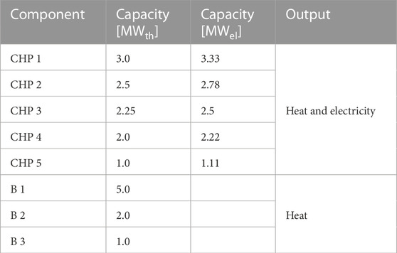
TABLE 1. Overview of the components of the multi-energy system, the installed capacities, and their thermal (th) and electricity (el) output. CHP: combined heat-and-power units; B: gas-driven boilers.

The case study aims to show how the proposed method can be used to decide on storage investments while accounting for the balancing-power market. Based on the investment decisions, we investigate the operational implications of heat storage for providing flexibility in the balancing-power market. Furthermore, the additional economic benefit of storage for providing flexibility is quantified for the studied multi-energy system.

To examine the benefit of investing in heat storage, we model a typical day with time steps of hourly resolution. This typical day approximates the market opportunities on the day-ahead market and balancing-power market, as well as the operational requirements for the multi-energy system. The typical day takes into account an hourly time series of electricity and heat demands. To select a typical day from the yearly time series by Baumgärtner et al. (2019b), we use hierarchical clustering based on the TSAM tool (Kotzur et al., 2018). The hourly demands for electricity and heat show a typical night and day pattern with low demands during nighttime and high demands during business hours (cf. Supplementary Appendix S3; Supplementary Appendix Figure S2).

The multi-energy system is able to offer flexibility to the balancing-power market. In our case study, we consider the German market for minute reserve as of August 2019. The studied market design incorporates all features of the stochastic process, such as capacity prices, energy prices, and separate marketing of positive and negative balancing power. In addition, we assume that the multi-energy system can provide balancing power within the required activation time of 15 min. We assume that in each hourly time step, either no request or a request of positive or negative balancing power occurs. Thus, the case study uses an hourly resolution to resolve operations. Since balancing power needs to be offered in time slices of 4 hours, we derive constant capacity prices, energy prices, and request probabilities for each time slice of 4 hours (cf. Supplementary Appendix S3; Supplementary Appendix Table S2).

We use market data for the period of August 2019–July 2020 for the day-ahead market and balancing-power market. The data of the balancing-power market are prepared similar to those in Muche et al. (2016) and Leenders et al. (2019) to obtain capacity prices ${\mathrm{p}}_t^{\mathrm{c}\mathrm{p},+/-}$, energy prices ${\mathrm{p}}_t^{\mathrm{e}\mathrm{p},+/-}$, and request probabilities π_{pos/ neg}. For this purpose, the mean capacity prices from Regelleistung.net (2021) are averaged by time slices. For each time slice, the energy price is calculated as the mean energy price of all quarter hours with the request of balancing power. The request probability is derived as quarter hours with the request of positive/negative balancing power divided by all quarter hours within a time slice. Additionally, we assume a maximum amount of 10 MW of positive and negative balancing power that can be offered to the balancing-power market. Since the German market for balancing-power capacity allows balancing power to be offered at time slices of 4 hours, we assume that balancing power must be offered for 4-hour time slices.

The multi-energy system sells and purchases electricity on the day-ahead market. The day-ahead market is represented by hourly varying electricity prices. We choose the electricity prices from Bundesnetzagentur (2021) for the same period (August 2019–July 2020) and select a typical day with hierarchical clustering using the TSAM package (Kotzur et al., 2018). Furthermore, we assume a difference between the electricity prices for selling and purchasing to account for carbon taxes (Bauer et al., 2022) and levies (Bundesnetzagentur, 2021) within the prices. Ultimately, Table 2 contains the overview of the case study parameters with average values and the respective data sources. We model the case study using the SecMOD MILP framework (Reinert et al., 2023).

TABLE 2

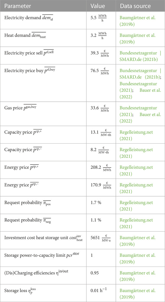
TABLE 2. Average input parameters for the case study, including data sources.

Following this, we consider the flexibilization of the multi-energy system using one typical day. The results based on four typical days are shown in Supplementary Appendix S4, yielding similar results. While the optimization problems with one typical day take a maximum of a few minutes to solve, four typical days already take more than 1 hour computational time. Flexibilization is achieved by a retrofit with a heat storage unit. Thus, in the following section, we examine the benefits of investment in the heat storage unit. Therefore, we consider five cases: the case (DAM) represents the base case with sole participation in the day-ahead market, while the case (DAM, BPM) takes into account the additional participation in the balancing-power market. Both cases (DAM) and (DAM, BPM) do not consider additional investment in the heat storage unit. The case (DAM, STOR) allows for investment in the storage unit but only considers participation in the day-ahead market. Since participation in the balancing-power market introduces inherent uncertainty, we examine the range of the additional advantages to market flexibility with the cases (SAME) and (FLEXIBLE). The case (SAME) allows for investment in the heat storage unit with formulation same; the case (FLEXIBLE) allows for investment in the heat storage unit with formulation flexible.

3.2 Flexibilization of the multi-energy system with the heat storage unit

Investment in a heat storage unit with participation in the balancing-power market leads to the largest cost savings. In the case (SAME), savings of 5.5% are expected, while the case (FLEXIBLE) indicates a cost reduction of 16.9% compared to the base case (DAM) (Figure 3). The additional participation in the balancing-power market in case (DAM, BPM) saves 3.0%, whereas the additional heat storage unit in case (DAM, STOR) enables savings of 1.7% compared to the base case (DAM). Thus, the heat storage unit enhances the flexibility of the multi-energy system with major benefits from the participation in the balancing-power market.

FIGURE 3

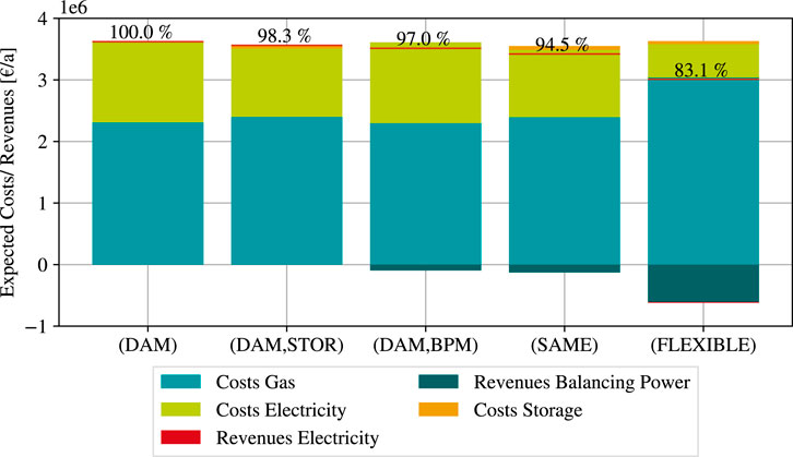
FIGURE 3. Annual costs and revenues with investment in the heat storage unit and/or additional participation in the balancing-power market. The relative total annualized costs, shown as a number above the bar, are referenced to the base case (DAM) with sole participation in the day-ahead market. At each bar, the red line indicates the total costs as the sum of costs and revenues.

In the case (SAME), costs are saved in the day-ahead market and in the balancing-power market. In the balancing-power market, investment in the heat storage unit facilitates the utilization of negative flexibility. Compared to the case (DAM, BPM), the additional heat storage unit of 11.0 MWh increases the provision of negative balancing power (Table 3): 3.5 MW negative balancing power is offered on average in case (SAME), while only 2.7 MW negative balancing power is offered on average in case (DAM, BPM). However, no positive balancing power is provided in both cases (SAME) and (DAM, BPM). Thus, the heat storage unit shifts the heat demands such that the operation of the CHP units is no more fixed to the heat demands. This shift enables the provision of more negative balancing power: if no balancing power is requested, the CHP units run at higher loads, thus having more negative flexibility. At the same time, the additional heat production from co-generation charges the heat storage (Figure 4). Both cases (SAME) and (DAM, BPM) offer no positive balancing power, since self-production of electricity is economically attractive in both cases. Thus, the CHP units cover electricity and heat demands rather than being utilized for the provision of positive balancing power.

TABLE 3

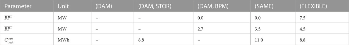
TABLE 3. Average amount of positive balancing power $\overline{B{P}^{+}}$, negative balancing power $\overline{B{P}^{-}}$, and heat storage capacity $C_{\text{heat}}^{\text{new}}$ for the cases (DAM), (DAM, STOR), (DAM, BPM), (SAME), and (FLEXIBLE).

FIGURE 4

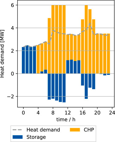
FIGURE 4. Operation of the multi-energy system in the case (SAME) in the no-request scenario for covering the time-varying heat demand (gray line). A positive value corresponds to a heat supply, and a negative value corresponds to a heat demand by the units.

The case (FLEXIBLE) with participation in the balancing-power market and investments in the flexible heat storage unit enables the largest cost savings of almost 16.9%. In this case, almost no electricity is purchased or sold on the day-ahead market. Since overproduction via the heat storage unit is possible, the CHP units of the multi-energy system are even more flexibilized. Therefore, the storage unit enables the electricity-driven operation of the CHP units: the electricity demand determines the operation of the CHP units. Subsequently, the CHP units are not restricted to strictly follow the heat demand (Figure 5). Electricity-driven operation enables the provision of positive balancing power: on average, 4.5 MW of positive balancing power and 7.5 MW of negative balancing power are provided (Table 3). Since the provision of balancing power corresponds nearly to the entire capacity of the multi-energy system’s electricity output, the flexibility of the multi-energy system is, therefore, entirely marketed on the balancing-power market in the case (FLEXIBLE). Overall, the case study indicates that in both cases (SAME) and (FLEXIBLE) the investment in a heat storage unit is beneficial. However, in the case (SAME), a larger heat storage unit of 11 MWh is built compared to the case (FLEXIBLE) with 8.8 MWh, as the case (FLEXIBLE) allows for overproduction. Here, we can thus observe a trade-off between overproduction and storage for the cases (SAME) and (FLEXIBLE): In case (SAME), excess heat needs to be stored, whereas storing excess heat is only partially beneficial in case (FLEXIBLE) due to the possibility of overproduction. As a result, less excess heat is stored in case (FLEXIBLE), and thus, a smaller heat storage unit is built.

FIGURE 5

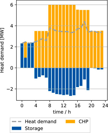
FIGURE 5. Operation of the multi-energy system in the case (FLEXIBLE) in the no-request scenario for covering the time-varying heat demand (gray line). A positive value corresponds to a heat supply, and a negative value corresponds to a heat demand by the units.

The case (DAM, STOR) with investment in the heat storage unit and sole participation in the day-ahead market leads to savings of approximately 1.7%. The heat storage unit exploits the time-dependent electricity prices of the day-ahead market: at times with high electricity prices, self-production of electricity is beneficial, and the electricity demand is covered with CHP units, while heat from co-generation provides the heat demand and charges the heat storage unit. At times with low electricity prices, electricity is purchased on the day-ahead market. In these hours, the heat demand is covered by gas-driven boilers and by discharging the heat storage unit. Thus, electricity costs are significantly reduced, while gas costs are modestly higher.

Additional participation in the balancing-power market without investment in storage units leads to savings of approximately 3.0% in case (DAM, BPM). In this case (DAM, BPM), the multi-energy system is operated in a similar way as in the case (DAM): if no balancing power is requested, the case (DAM, BPM) purchases the same amount of electricity on the day-ahead market and consumes the same amount of gas as the case (DAM). However, the case (DAM, BPM) also markets negative flexibility on the balancing-power market if available. Therein, the supply of negative flexibility is linked to heat demands, since the multi-energy system offers the lowest amount of balancing power during nighttime hours at low heat demands (time slice 0–4 h) and the highest amount of balancing power in the morning at high heat demands (time slice 8–12 h).

The investment in the heat storage unit makes the operation of the multi-energy system more flexible. Thus, more balancing power can be provided in more beneficial time slices: in the case (FLEXIBLE), the heat storage unit allows all flexibility to be marketed, so the amount of balancing power provided throughout the day is significantly higher compared to that in the case (DAM, BPM) (Figure 7).

FIGURE 7

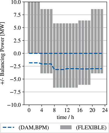
FIGURE 7. Positive and negative balancing power provided in the case (FLEXIBLE) compared to the case (DAM, BPM).

In the case (SAME), balancing power is provided in different time slices compared to the case (DAM, BPM) (Figure 6). In this case (DAM, BPM), balancing power is provided relatively evenly throughout the day. In case (SAME), however, no negative balancing power is offered in time slice 0–4 h, while more than 6 MW is offered in time slice 8–12 h and more than 5 MW in time slice 16–20 h (Figure 6). In both time slices, capacity prices, energy prices, and electricity prices are higher than those in time slice 0–4 h. Thus, the heat storage unit enables offering balancing power at more economical time slices. The proposed method takes not only the prices at the balancing-power market into account but also the opportunity costs from the day-ahead market. Overall, the heat storage improves, in both cases (SAME) and (FLEXIBLE), the operation of the multi-energy system to cover the time-varying heat demands (cf. Figures 4, 5)

FIGURE 6

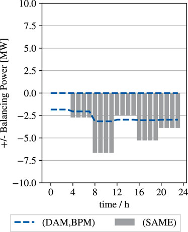
FIGURE 6. Positive and negative balancing power provided in the case (SAME) compared to the case (DAM, BPM).

Comparing the different cases shows that investment in heat storage units makes the multi-energy system more flexible. For the largest savings, flexibility is offered in the balancing-power market. Therefore, the formulations same and flexible specify a range of savings through flexibility marketing. Same allows flexibility to be shifted toward more beneficial time steps, while the overproduction of heat in formulation flexible facilitates further flexibilization of the CHP units of the multi-energy system. Note that despite possible overproduction, a request for balancing power is unlikely (cf. request probabilities in Table 2).

3.3 Investment in heat storage units for varying heat demands

The method shows that the heat storage unit facilitates cost savings in the balancing-power market for the considered multi-energy system. Since the CHP units couple the electricity supply with the heat supply, the flexibility of the multi-energy system also depends on the heat demands. Therefore, this section analyzes the relative savings by investment in the heat storage unit (Figure 8) and the optimal size of the storage unit for varying heat demands (Figure 9). We vary the heat demand for the average day by scaling the heat demand between 25% and 300% of the initial heat demand. The size of the heat supply units, i.e., the boilers and CHP units, remains the same (cf. Table 1). Therefore, we investigate the relative savings related to the base case (DAM) as the cost difference between the base case (DAM) and any other case (Figure 8).

FIGURE 8

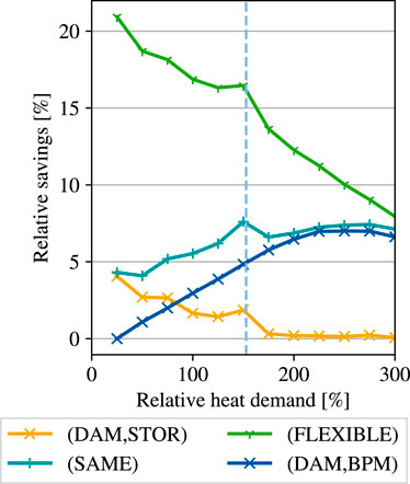
FIGURE 8. Additional relative savings for varying heat demands with investment in the heat storage unit and/or additional participation in the balancing-power market for the cases (DAM, BPM), (DAM, STOR), (SAME), and (FLEXIBLE). In each case, the additional savings are related to the objective function when solely participating in the day-ahead market.

FIGURE 9

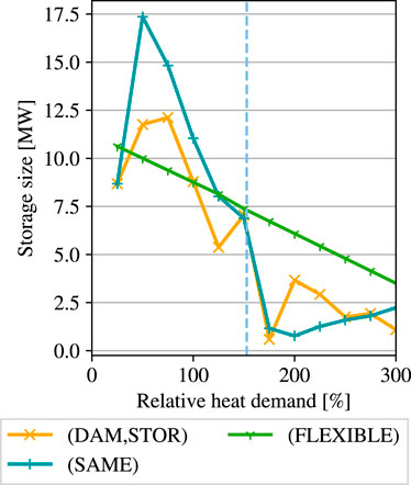
FIGURE 9. Optimal heat storage size for varying relative heat demands for the cases (DAM, STOR), (SAME), and (FLEXIBLE). With a relative heat demand of approximately 160%, the ratio of heat to electricity demand is approximately the same as the ratio of heat to electricity output of the multi-energy system.

For all relative heat demands, the investment in the heat storage unit, in combination with the provision of balancing power, leads to the largest savings. For low relative heat demands (25%–150%), the savings compared to the base case (DAM) range between 4.1% (SAME) and 20.9% (FLEXIBLE); for high relative heat demands (175%–300%), the savings range between 4.3% (SAME) and 4.4% (FLEXIBLE). Higher relative heat demands lead to larger savings in the case (DAM, BPM) with sole participation in the balancing-power market, whereas higher relative heat demands diminish the savings in the case (DAM, STOR). Hence, the advantage of heat storage decreases as the relative heat demands increase. Therefore, increasing heat demands no longer restrict the multi-energy system’s flexibility.

The savings from an investment in the heat storage unit thus depend on the relative heat demand. If no heat storage is available, the heat demands limit the flexibility of the CHP units at low relative heat demands due to the coupling of electricity and heat production. Therein, the multi-energy system operates as a heat-driven system: the maximum electricity output of the CHP units is restricted by the heat demands. To overcome this restriction, relatively large heat storage units are built at low relative heat demands (Figure 9) since the shift of heat among different time steps is highly beneficial. In case (DAM, STOR), the heat storage unit is used to shift the heat demand, such that self-production of electricity increases in hours of high electricity prices. Compared to the case (DAM, STOR), the case (SAME) builds larger heat storage units to enable additional flexibility for the provision of balancing power, while the case (FLEXIBLE) allows for overproduction leading to smaller heat storage units.

At the threshold of 160% relative heat demand, the ratio of heat to electricity demand is exactly the same as the ratio of heat to electricity supply (blue dashed vertical line in Figures 8, 9). For relative heat demands larger than the threshold of 160%, only small heat storage units are economically optimal, showing diminishing additional benefit by investment in the heat storage unit. For these demands, most flexibility of the CHP units can already be used without the heat storage unit. The CHP units can be operated electricity-driven: the heat demands do not limit the operation of the CHP units, but the electricity supply determines the operation of the units. In addition, gas-driven boilers supply the heat. Thus, for larger relative heat demands, small heat storage units are built in cases (DAM, STOR) and (SAME) since only a small part of the heat demand needs to be shifted for further flexibility. However, the case (FLEXIBLE) allows for overproduction. To utilize this additional flexibility, larger heat storage sizes are necessary compared to the cases (DAM, STOR) and (SAME).

In conclusion, the heat-driven and electricity-driven operation has a substantial impact on the available flexibility of the multi-energy system. Therefore, the trade-off between overproduction and storage changes both the storage sizes and the qualitative relationship of the storage size between the cases (SAME), (FLEXIBLE), and (DAM, STOR). Consequentially, the heat demands have a substantial impact on the optimal deployment of the heat storage unit.

3.4 Discussion

The results of our case study show that the investment in the heat storage unit makes the multi-energy system more flexible in all cases. The heat storage unit allows an increase in the offered amount of balancing power, increasing the economic benefit from participation in the balancing-power market. The case study, thus, supports the findings of Srinivasan et al. (2023) that storage is one key to enhancing the flexibility of multi-energy systems.

However, the additional benefit of the storage units is found to vary significantly with the relative heat demand: for low relative heat demands, the studied multi-energy system operates as a heat-driven system. In this case, larger storage sizes are particularly valuable to shift heat to gain flexibility. For electricity-driven multi-energy systems, smaller storage units are found to be sufficient to utilize the flexibility of the multi-energy system. Thus, the proposed method is able to consider the complex trade-off between long-term investment decisions in storage for flexibility in short-term operation. Therefore, the method is likely a good decision-support tool also in other cases.

In future work, the method could be studied on a broader set of multi-energy systems to allow for more general conclusions and design guidelines. An important aspect is that the present case study focuses on retrofitting a multi-energy system that relies on natural gas as a fuel input. However, with the ongoing energy transition, these systems should increasingly rely on renewable energy sources, i.e., green fuels or electricity-driven units, as discussed in the introduction. In addition, for these systems, the flexibility potential needs to be studied. Still, heat storage is expected to remain a potentially valuable flexibility option, and thus, our method should also provide a valuable tool for the optimal system design of renewable energy systems.

A further shortcoming is that our case study assumes a power-to-capacity limit of 1. If this limit is reduced, the economic performance of storage systems may also be worse since the short-term provision of balancing power may prefer higher storage power. In addition, for cases with lower power-to-capacity ratios, our method could help determine whether such storage systems are still useful.

Overall, the method focuses on the operational uncertainties from the provision of balancing power. However, other uncertainties also affect the economic performance of multi-energy systems, such as forecast uncertainties in electricity markets (Srinivasan et al., 2023) and demand uncertainties (Mavromatidis et al., 2018). These uncertainties, therefore, may also significantly impact the optimal design. Modeling of additional flexibility potentials, e.g., at the intraday market (Teichgraeber and Brandt, 2020; Nolzen et al., 2022), could show further opportunities for multi-energysystems.

4 Conclusion

This work presents a method to integrate the balancing-power market into a design optimization of multi-energy systems. As design optimization with the balancing-power market yields a complex stochastic optimization problem, we present a simple approach for considering the balancing-power market.

The balancing-power market introduces inherent uncertainty to the optimization problem. To reflect this uncertainty, we use stochastic programming. However, the stochastic optimization would grow exponentially with time-coupling storage. To model time-coupling storage within the stochastic optimization, we present two methods that both derive feasible storage levels: formulation same considers the same storage level regardless of the request for balancing power. Formulation flexible considers the lowest storage level for the next time step, thus allowing for overproduction in this formulation that results in a loss.

The method is evaluated in a case study of a multi-energy system participating in the balancing-power market in addition to the day-ahead market. The multi-energy system comprising CHP units and gas-driven boilers is retrofitted with a heat storage unit.

The method indicates that an additional heat storage unit increases flexibility. More balancing power can be offered, leading to cost reductions between 5.5% and 16.9% compared to a case with sole participation in the day-ahead market. As we vary heat demands in a sensitivity analysis, the benefits and the optimal sizing of the heat storage vary significantly: at low heat demands, the multi-energy system operates as a heat-driven system, resulting in comparatively large storage units. At higher heat demands, small heat storage units are economically optimal as the multi-energy system can operate as an electricity-driven system without being limited by heat demands.

Future research could focus on integrating multiple market opportunities (e.g., the intraday market) or providers (e.g., energy-intense processes) to utilize flexibility in design optimization. Overall, this paper provides a method to optimally design storage for balancing power market participation and, thus, flexibility provision by multi-energy systems. This flexibilization supports the energy transition to integrate more renewables into the energy system.

Data availability statement

The original contributions presented in the study are included in the article/Supplementary Material; further inquiries can be directed to the corresponding author.

Author contributions

NN: writing—original draft, conceptualization, methodology, software, investigation, data curation, visualization, and project administration. LL: conceptualization, methodology, visualization, writing—review and editing, supervision, and funding acquisition. AB: writing—review and editing, conceptualization, supervision, resources, and funding acquisition. All authors contributed to the article and approved the submitted version.

Funding

This study was funded by the German Federal Ministry of Economic Affairs and Energy (Ref. No. 03EI1015A). LL and AB’s work was sponsored by the Swiss Federal Office of Energy’s “SWEET” programme and performed in the “PATHFNDR” consortium. Open access funding was provided by ETH Zurich.

Conflict of interest

The authors declare that the research was conducted in the absence of any commercial or financial relationships that could be construed as a potential conflict of interest.

Publisher’s note

All claims expressed in this article are solely those of the authors and do not necessarily represent those of their affiliated organizations, or those of the publisher, the editors, and the reviewers. Any product that may be evaluated in this article, or claim that may be made by its manufacturer, is not guaranteed or endorsed by the publisher.

Supplementary material

The Supplementary Material for this article can be found online at: https://www.frontiersin.org/articles/10.3389/fenrg.2023.1225564/full#supplementary-material

References

Angenendt, G., Zurmühlen, S., Figgener, J., Kairies, K.-P., and Sauer, D. U. (2020). Providing frequency control reserve with photovoltaic battery energy storage systems and power-to-heat coupling. Energy 194, 116923. doi:10.1016/j.energy.2020.116923

CrossRef Full Text | Google Scholar

Bauer, T., Prenzel, M., Klasing, F., Franck, R., Lützow, J., Perrey, K., et al. (2022). Ideal–typical utility infrastructure at chemical sites – definition, operation and defossilization. Chem. Ing. Tech. 94, 840–851. doi:10.1002/cite.202100164

CrossRef Full Text | Google Scholar

Baumgärtner, N., Bahl, B., Hennen, M., and Bardow, A. (2019a). RiSES3: rigorous synthesis of energy supply and storage systems via time-series relaxation and aggregation. Comput. Chem. Eng. 127, 127–139. doi:10.1016/j.compchemeng.2019.02.006

CrossRef Full Text | Google Scholar

Baumgärtner, N., Delorme, R., Hennen, M., and Bardow, A. (2019b). Design of low-carbon utility systems: exploiting time-dependent grid emissions for climate-friendly demand-side management. Appl. Energy 247, 755–765. doi:10.1016/j.apenergy.2019.04.029

CrossRef Full Text | Google Scholar

Birge, J. R., and Louveaux, F. (2011). Introduction to stochastic programming. New York, NY: Springer New York. doi:10.1007/978-1-4614-0237-4

CrossRef Full Text | Google Scholar

Bischi, A., Taccari, L., Martelli, E., Amaldi, E., Manzolini, G., Silva, P., et al. (2014). A detailed MILP optimization model for combined cooling, heat and power system operation planning. Energy 74, 12–26. doi:10.1016/j.energy.2014.02.042

CrossRef Full Text | Google Scholar

Bohlayer, M., Bürger, A., Fleschutz, M., Braun, M., and Zöttl, G. (2021). Multi-period investment pathways - modeling approaches to design distributed energy systems under uncertainty. Appl. Energy 285, 116368. doi:10.1016/j.apenergy.2020.116368

CrossRef Full Text | Google Scholar

Bohlayer, M., Fleschutz, M., Braun, M., and Zöttl, G. (2020). Energy-intense production-inventory planning with participation in sequential energy markets. Appl. Energy 258, 113954. doi:10.1016/j.apenergy.2019.113954

CrossRef Full Text | Google Scholar

Bringedal, A. S., Søvikhagen, A.-M. L., Aasgård, E. K., and Fleten, S.-E. (2021). Backtesting coordinated hydropower bidding using neural network forecasting. Energy Syst. 29, 1758. doi:10.1007/s12667-021-00490-4

CrossRef Full Text | Google Scholar

Brouwer, A. S., van den Broek, M., Seebregts, A., and Faaij, A. (2014). Impacts of large-scale Intermittent Renewable Energy Sources on electricity systems, and how these can be modeled. Renew. Sustain. Energy Rev. 33, 443–466. doi:10.1016/j.rser.2014.01.076

CrossRef Full Text | Google Scholar

Bundesnetzagentur | SMARD.de (2021b). SMARD - Strommarktdaten. Available at: https://smard.de/ (Accessed May 05, 2022).

Google Scholar

Bundesnetzagentur (2021a). Monitoringbericht 2021: Monitoringbericht gemäß § 63 abs. 3 i. V. m. § 35 EnWG und § 48 Abs. 3 i. V. m. § 53 Abs. 3 GWB.

Google Scholar

Goderbauer, S., Comis, M., and Willamowski, F. J. (2019). The synthesis problem of decentralized energy systems is strongly NP-hard. Comput. Chem. Eng. 124, 343–349. doi:10.1016/j.compchemeng.2019.02.002

CrossRef Full Text | Google Scholar

Guelpa, E., Bischi, A., Verda, V., Chertkov, M., and Lund, H. (2019). Towards future infrastructures for sustainable multi-energy systems: A review. Energy 184, 2–21. doi:10.1016/j.energy.2019.05.057

CrossRef Full Text | Google Scholar

Hoettecke, L., Schuetz, T., Thiem, S., and Niessen, S. (2022). Technology pathways for industrial cogeneration systems: optimal investment planning considering long-term trends. Appl. Energy 324, 119675. doi:10.1016/j.apenergy.2022.119675

CrossRef Full Text | Google Scholar

Hoffmann, M., Kotzur, L., Stolten, D., and Robinius, M. (2020). A review on time series aggregation methods for energy system models. Energies 13, 641. doi:10.3390/en13030641

CrossRef Full Text | Google Scholar

Iea, I. E. A. (2021). Renewables 2021 - analysis and forecast to 2026.

Google Scholar

Javanshir, N., Syri, S., Tervo, S., and Rosin, A. (2023). Operation of district heat network in electricity and balancing markets with the power-to-heat sector coupling. Energy 266, 126423. doi:10.1016/j.energy.2022.126423

CrossRef Full Text | Google Scholar

Kotzur, L., Markewitz, P., Robinius, M., and Stolten, D. (2018). Impact of different time series aggregation methods on optimal energy system design. Renew. Energy 117, 474–487. doi:10.1016/j.renene.2017.10.017

CrossRef Full Text | Google Scholar

Kumbartzky, N., Schacht, M., Schulz, K., and Werners, B. (2017). Optimal operation of a CHP plant participating in the German electricity balancing and day-ahead spot market. Eur. J. Operational Res. 261, 390–404. doi:10.1016/j.ejor.2017.02.006

CrossRef Full Text | Google Scholar

Lahrsen, I.-M., Hofmann, M., and Müller, R. (2022). Flexibility of epichlorohydrin production—increasing profitability by demand response for electricity and balancing market. Processes 10, 761. doi:10.3390/pr10040761

CrossRef Full Text | Google Scholar

Leenders, L., Bahl, B., Hennen, M., and Bardow, A. (2019). Coordinating scheduling of production and utility system using a Stackelberg game. Energy 175, 1283–1295. doi:10.1016/j.energy.2019.03.132

CrossRef Full Text | Google Scholar

Leenders, L., Starosta, A., Baumgärtner, N., and Bardow, A. (2020). “Integrated scheduling of batch production and utility systems for provision of control reserve,” in Proceedings of ECOS 2020 - 33rd international conference on efficiency, cost, optimization, simulation and environmental impact of energy systems (Osaka), 712–723. doi:10.3929/ethz-b-000423722

CrossRef Full Text | Google Scholar

Mavromatidis, G., Orehounig, K., and Carmeliet, J. (2018). Design of distributed energy systems under uncertainty: A two-stage stochastic programming approach. Appl. Energy 222, 932–950. doi:10.1016/j.apenergy.2018.04.019

CrossRef Full Text | Google Scholar

Muche, T., Höge, C., Renner, O., and Pohl, R. (2016). Profitability of participation in control reserve market for biomass-fueled combined heat and power plants. Renew. Energy 90, 62–76. doi:10.1016/j.renene.2015.12.051

CrossRef Full Text | Google Scholar

Nolzen, N., Ganter, A., Baumgärtner, N., Leenders, L., and Bardow, A. (2022). Where to market flexibility? Optimal participation of industrial energy systems in balancing-power, day-ahead, and continuous intraday electricity markets. arXiv preprint. doi:10.48550/arXiv.2212.12507

CrossRef Full Text | Google Scholar

Nolzen, N., Leenders, L., and Bardow, A. (2021). “Flexibility-expansion planning for enhanced balancing-po market participation of decentralized energy systems,” in 31st European symposium on computer aided process engineering (Elsevier), 50, 1841–1846. of Computer Aided Chemical Engineering. doi:10.1016/B978-0-323-88506-5.50285-0

CrossRef Full Text | Google Scholar

Ocker, F., and Ehrhart, K.-M. (2017). The “German Paradox” in the balancing power markets. Renew. Sustain. Energy Rev. 67, 892–898. doi:10.1016/j.rser.2016.09.040

CrossRef Full Text | Google Scholar

Prenzel, M., Klasing, F., Franck, R., Perrey, K., Trautmann, J., Reimer, A., et al. (2023). The potential of thermal energy storage for sustainable energy supply at chemical sites. Proc. Int. Renew. Energy Storage Conf. (IRES 2022) (Düsseldorf) 16, 383–400. doi:10.2991/978-94-6463-156-2_25

CrossRef Full Text | Google Scholar

Rancilio, G., Rossi, A., Falabretti, D., Galliani, A., and Merlo, M. (2022). Ancillary services markets in europe: evolution and regulatory trade-offs. Renew. Sustain. Energy Rev. 154, 111850. doi:10.1016/j.rser.2021.111850

CrossRef Full Text | Google Scholar

Regelleistung.net (2021). aFRR datencenter: Regelleistungsmarkt (Accessed on May 10, 2021).

Google Scholar

Reinert, C., Nolzen, N., Frohmann, J., Tillmanns, D., and Bardow, A. (2023). Design of low-carbon multi-energy systems in the SecMOD framework by combining MILP optimization and life-cycle assessment. Comput. Chem. Eng. 172, 108176. doi:10.1016/j.compchemeng.2023.108176

CrossRef Full Text | Google Scholar

Roh, K., Brée, L. C., Perrey, K., Bulan, A., and Mitsos, A. (2019). Flexible operation of switchable chlor-alkali electrolysis for demand side management. Appl. Energy 255, 113880. doi:10.1016/j.apenergy.2019.113880

CrossRef Full Text | Google Scholar

Sass, S., Faulwasser, T., Hollermann, D. E., Kappatou, C. D., Sauer, D., Schütz, T., et al. (2020). Model compendium, data, and optimization benchmarks for sector-coupled energy systems. Comput. Chem. Eng. 135, 106760. doi:10.1016/j.compchemeng.2020.106760

CrossRef Full Text | Google Scholar

Sass, S., and Mitsos, A. (2019). Optimal operation of dynamic (energy) systems: when are quasi-steady models adequate? Comput. Chem. Eng. 124, 133–139. doi:10.1016/j.compchemeng.2019.02.011

CrossRef Full Text | Google Scholar

Schäfer, P., Daun, T. M., and Mitsos, A. (2020). Do investments in flexibility enhance sustainability? A simulative study considering the German electricity sector. AIChE J. 66, 1. doi:10.1002/aic.17010

CrossRef Full Text | Google Scholar

Schäfer, P., Westerholt, H. G., Schweidtmann, A. M., Ilieva, S., and Mitsos, A. (2019). Model-based bidding strategies on the primary balancing market for energy-intense processes. Comput. Chem. Eng. 120, 4–14. doi:10.1016/j.compchemeng.2018.09.026

CrossRef Full Text | Google Scholar

Schlachter, U., Worschech, A., Diekmann, T., Hanke, B., and von Maydell, K. (2020). Optimised capacity and operating strategy for providing frequency containment reserve with batteries and power-to-heat. J. Energy Storage 32, 101964. doi:10.1016/j.est.2020.101964

CrossRef Full Text | Google Scholar

Srinivasan, A., Wu, R., Heer, P., and Sansavini, G. (2023). Impact of forecast uncertainty and electricity markets on the flexibility provision and economic performance of highly-decarbonized multi-energy systems. Appl. Energy 338, 120825. doi:10.1016/j.apenergy.2023.120825

CrossRef Full Text | Google Scholar

Teichgraeber, H., and Brandt, A. R. (2020). Optimal design of an electricity-intensive industrial facility subject to electricity price uncertainty: stochastic optimization and scenario reduction. Chem. Eng. Res. Des. 163, 204–216. doi:10.1016/j.cherd.2020.08.022

CrossRef Full Text | Google Scholar

Varelmann, T., Erwes, N., Schäfer, P., and Mitsos, A. (2022). Simultaneously optimizing bidding strategy in pay-as-bid-markets and production scheduling. Comput. Chem. Eng. 157, 107610. doi:10.1016/j.compchemeng.2021.107610

CrossRef Full Text | Google Scholar

Voll, P. (2014). Automated optimization-based synthesis of distributed energy supply systems: Aachen, Techn. Hochsch., Diss. 1 of Aachener Beiträge zur Technischen Thermodynamik (Aachen: Hochschulbibliothek der Rheinisch-Westfälischen Technischen Hochschule Aachen).

Google Scholar

Zhang, Q., Grossmann, I. E., Heuberger, C. F., Sundaramoorthy, A., and Pinto, J. M. (2015). Air separation with cryogenic energy storage: optimal scheduling considering electric energy and reserve markets. AIChE J. 61, 1547–1558. doi:10.1002/aic.14730

CrossRef Full Text | Google Scholar

Zhang, R., Sun, H., Li, G., Jiang, T., Li, X., Chen, H., et al. (2023). Reserve provision of combined-cycle unit in joint day-ahead energy and reserve markets. Appl. Energy 336, 120812. doi:10.1016/j.apenergy.2023.120812

CrossRef Full Text | Google Scholar

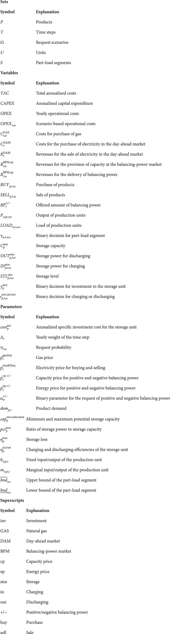
Nomenclature