A model for identifying the feeder-transformer relationship in distribution grids using a data-driven machine-learning algorithm

With the increasing demand for reliable power supply and the widespread integration of distributed energy sources, the topology of distribution networks is subject to frequent changes. Consequently, the dynamic alterations in the connection relationships between distribution transformers and feeders occur frequently, and these changes are not accurately monitored by grid companies in real-time. In this paper, we present a data-driven machine learning approach for identifying the feeder-transformer relationship in distribution networks. Initially, we preprocess the collected three-phase voltage magnitude data of distribution transformers, addressing data quality and enhancing usability through three-phase voltage normalization. Subsequently, we derive the correlation coefficient calculations between distribution transformers, as well as between distribution transformers and feeders. To tackle the challenging task of determining the correlation coefficient threshold, we propose a multi-feature fusion approach. We extracted additional features from the feeders and combined them with the correlation coefficients to create a feature matrix. Machine learning algorithms were then applied to calculate the results. Through experimentation on a real distribution network in Jiangxi province, we demonstrated the effectiveness of the proposed method. When compared to other approaches, our method achieved outstanding results with an F1 score of 0.977, indicating high precision and recall. The precision value was 0.973 and the recall value was 0.981. Importantly, our method eliminates the need for additional measurement installations, as the required data can be obtained using existing collection devices. This significantly reduces the application cost associated with implementing our approach.

1 Introduction

The distribution network serves as the crucial link in the power delivery chain to end-users. It’s safe and stable operation has a direct impact on the reliability and quality of power supply to customers (Hock et al., 2018; Naik et al., 2018). Furthermore, an accurate representation of the distribution network topology is essential for various activities such as line loss calculations, tide analysis, grid transformation, and outage restoration. Achieving an accurate distribution network topology forms the basis for intelligent operation, maintenance, and dispatching of the distribution network, ultimately influencing customer satisfaction (Krsman and Saric, 2017).

In practical operation, the distribution network undergoes frequent restructuring due to various factors such as the addition of new equipment, integration of distributed energy sources, and load switching. These dynamic changes pose significant challenges in obtaining real-time and accurate information about the distribution network’s topology (Zhao et al., 2021).

The identification of the distribution network’s topology involves several aspects, including determining the line relationships between distribution transformers (referred to as the feeder-transformer relationship), identifying the phase sequence of customers, and associating distribution transformers with specific customers. In China, the distribution network covers a large power supply range, and its complex topology has not been fully addressed through intelligent reforms. While significant progress has been made in installing intelligent devices for data collection in recent years (Van and Poll, 2019), the data collected by smart meters remains limited, particularly considering the extensive coverage of low-voltage distribution networks. Therefore, the identification of phase sequences for users in the distribution network topology may already meet the requirements. However, there are limitations in accurately identifying the feeder-transformer relationship. This relationship is crucial for load dispatch, line loss calculation, power restoration, fault location assessment, and other important aspects of the low-voltage distribution network (Song et al., 2021). Grid companies have made efforts to monitor the distribution network topology, creating and storing topology maps in a Geographic Information System (GIS) during network construction. However, due to operational changes, load adjustments, and other factors, timely updates of distribution topology changes to the GIS are not always feasible (Zhou et al., 2020a; Zhou et al., 2020b). Over time, differences emerge between the actual network operation and the topology stored in the GIS (Luan et al., 2013). Therefore, this paper focuses on studying the feeder-transformer relationship in the distribution network topology.

In traditional approaches, distribution network topology identification has relied on the verification of a priori information and hardware-based methods (Deka et al., 2018). The verification with a priori information involves using state quantities of switches or circuit breakers on the lines to generate correlation and collocation matrices for identifying the distribution network’s topology (Freitas and Costa, 2015). However, as mentioned earlier, the a priori knowledge of the distribution networks topology stored in the actual operating system may not be accurate. Consequently, relying solely on a priori knowledge for distribution network topology identification may not yield satisfactory results.

In hardware-based identification, a commonly used approach is to use a specialized signal injection device. This method involves using a micro-synchronous phase generator to inject high-frequency characteristic signals, which are then monitored and analyzed for topology recognition of the distribution network (Alam et al., 2014; Byun et al., 2018; Wu et al., 2021). However, this option requires substantial hardware support and manual analysis of the signals, resulting in time-consuming, inefficient, and costly processes, particularly for large-scale distribution networks. As a result, grid companies are often hesitant to adopt this approach.

The development of Supervisory Control and Data Acquisition (SCADA) systems and Advanced Measurement Infrastructure (AMI) has led to the installation of numerous data acquisition devices in the distribution network. This enables access to a wealth of operational data from the distribution network (Jielong et al., 2023). Taking advantage of the multiple measurement data obtained, data-driven approaches for distribution network topology identification have been widely proposed in recent years. These studies can be categorized into two main types: graph model-based approaches (Weng et al., 2017; Pappu et al., 2018; Liao et al., 2019; Deka et al., 2020; Gadelha et al., 2021) and data-driven approaches (Zhao et al., 2021).

In the graph model-based approach, Pappu et al. (2018) utilized principal component analysis in conjunction with graph theory to analyze load data collected by smart meters, enabling the inference of steady-state distribution network topology. Gadelha et al. (2021) combined graph theory, clustering, and Geographic Information System (GIS) techniques to analyze steady-state voltages, transformer loads, and line loads, ultimately determining the distribution network topology. Weng et al. (2017); Deka et al. (2020) proposed using a synchronous voltage measurement device to capture voltage data, which was further analyzed to obtain the topology. They employed a probabilistic graphical model to describe the statistical dependence between different voltage measurements, demonstrating that the estimation of line connectivity and grid topology in topology identification can be formulated as linear regression problems (Liao et al., 2019). Ji et al. (2019) proposed a graph theory approach based on real-time measurements to identify the topology of distribution networks, which does not require the use of circuit analysis methods. It has to use the covariance as well as the energy matrix K to find the maximum graph index to determine the topology. Gao et al. (2020) proposed a topology identification method based on knowledge graphs, which can overcome the drawbacks of online identification methods that require huge amounts of high-quality operational data and occupy communication channels. In general, the graph theory approach and the structure of the distribution network have a great degree of similarity. However, since the data originally presented in the system is wrong, the imported nodes and edges are also wrong when using graph theory. This will eventually lead to errors in the discriminatory results.

In the data-driven approach, Zhao et al. (2021) proposed a model that combines Principal Component Analysis (PCA) and Deep Belief Networks (DBN) to identify topology. This model extracts features using PCA and utilizes DBN to capture the nonlinear relationship between voltage amplitude and switchable connected binary states, enabling stable topology identification even in the presence of data quality issues and noise. Building upon this work, Zhao et al. (2021) presented a user phase recognition algorithm based on user classification, quadratic programming, and probability distribution. They further proposed a multidimensional calibration method for user phase identification in low-voltage distribution networks to handle data incompleteness. Liang et al. (2021) utilized Advanced Measurement Infrastructure (AMI) data and studied the topology identification of radial medium voltage distribution networks based on tide matching. García et al. (2023) developed a phase identification method based on Bayesian inference, using the load curve of the low-voltage distribution network as input. Srinivas and Wu. (2022) employed probabilistic and deterministic methods to identify topology and parameters using measured values from smart meters and micro-phase measurement units. They also determined the optimal installation location of the micro-phase measurement unit device. Tian et al. (2016) proposed a topology identification model based on Mixed Integer Quadratic Programming (MIQP), utilizing a weighted least squares (WLS) estimation method of measured residuals. Luan et al. (2015) demonstrated that correlation coefficients of voltage sequences can be used to evaluate the distance between energy meters, thereby determining their upstream and downstream locations. Cavraro et al. (2019) used smart inverters to detect the topology of the distribution network based on voltage deviations of the nodes, even when the load is unknown. Electrical tariffs (Kekatos et al., 2016), standard expressions for voltage drop (Deka et al., 2018), and voltage covariance matrices (Cavraro and Kekatos, 2019) have also been employed to measure topology. Luan et al. (2015) proposed a voltage correlation-based calibration method for the feeder-transformer relationship in distribution networks. Despite some promising results obtained from the mentioned research methods, there has been limited research specifically focusing on the feeder-transformer relationship, and challenges arising from data loss and voltage drop over long distances have not been adequately addressed.

In this paper, the three-phase voltage of the distribution transformer needs to be extracted, so the state of the distribution transformer is an important influencing factor in the identification of the feeder-transformer relationship. Badawi et al. (2022) presents comprehensive maintenance for power transformers aiming to diagnose transformer faults more accurately. Specifically, it aims to identify incipient faults in power transformer’s using what is known as dissolved gas analysis (DGA) with a new proposed integrated method. Accordingly, this proposed integrated DGA method could improve the overall accuracy by 93.6% compared to the existing DGA techniques. Ghoneim et al. (2021) Box-Behnken design (BBD) was used to introduce a prediction model of the breakdown voltage (VBD) for the transformer insulating oil in the presence of different barrier effects for point/plane gap arrangement with alternating current (AC) voltage. The findings illustrated the high accuracy and robustness of the proposed insulating oil breakdown voltage predictive model linked with diverse barrier effects. Darwish et al. (2022a) check the reliability of estimating the transformer’s Health index (HI) percentage based on the optical spectroscopy techniques. The HI percentages were estimated for the transformers simulated by these aged samples according to their DDP values. In the final analysis, this optical method has proven its potential in being a superior alternative to conventional techniques in estimating the transformer’s HI percentage. Darwish et al. (2022b) use Fourier Transform Infrared (FTIR) spectroscopy was employed to discriminate between the electrical and thermal faults that frequently happen in oil insulation. In the final analysis, it was obvious that the implementation of the optical method is considered a promising tool to monitor the faulted oil and distinguish between the electrical fault and the thermal one making the FTIR spectroscopy a superior alternative for DGA.

In addition, this paper utilizes various machine learning algorithms to enhance the identification of feeder-transformer relationships in distribution networks. Advanced machine learning methods can greatly influence the accuracy and effectiveness of the results. For instance, in the work conducted by Rahul et al. (2023), machine learning algorithms were employed to estimate long-term irradiation levels on a global scale. The paper showcased a diverse range of machine learning algorithms and compared their performance and results to determine the most suitable prediction algorithm. Furthermore, Rahul et al. (2022) also utilized machine learning algorithms for time series prediction analysis. Machine Learning algorithms such as Facebook (FB) Prophet and Extreme Gradient Boost (XGB) are used for predicting solar energy generation on a monthly and weekly basis. It concluded that the XGB model is efficient to forecast in terms of better prediction and better fitting than the FB prophet model. RMSE, MAPE, and MAE parameters are calculated to check the performance of the time series model.

In this paper, we propose a data-driven processing fused with machine learning (DDML) approach for identifying the feeder-transformer relationship in distribution networks. The main contributions of this work are as follows:

1) On the basis of addressing the errors caused by three-phase imbalance, we derived the calculation methods for the correlation coefficients between distribution transformers and between distribution transformers and feeders using the voltage drop formula and Ohm’s law. This is crucial for determining the relationship between feeders and transformers.

2) We proposed a multi-feature fusion approach to improve the accuracy of identification by incorporating multiple features in addition to the correlation coefficients.

3) To overcome the challenge of determining the optimal identification threshold solely based on correlation coefficients, we introduced a machine learning method for data mining, enabling accurate identification of the relationship between feeders and transformers.

4) we have conducted extensive experiments on a real distribution network, demonstrating the effectiveness of our proposed method. The results show high precision and recall values, indicating the robustness and reliability of our approach.

The rest of the paper is organized as follows: Section 2 describes the problem formulation as well as the feasibility. Section 3 describes the data pre-processing and the calculation of the voltage correlation. Algorithm models and their training are presented in Section 4. The comparison of the case study with other algorithms is presented in Section 5. Section 6 summarizes the full text.

2 Problem formulation

In practical operation, the distribution network undergoes adjustments to minimize network losses and balance the load, which leads to dynamic changes in the feeder-transformer relationship within the distribution network topology. Unfortunately, these changes are often not promptly recorded in the Geographic Information System (GIS) used by the staff, resulting in discrepancies between the actual feeder-transformer relationship and the recorded feeder-transformer relationship in the GIS system. This discrepancy can be seen in Figure 1, where T4 is shown connected to 10 kV feeder 1 in the GIS system, but in reality, it is connected to 10 kV feeder 2, causing errors in the feeder-transformer relationship. These issues significantly impact the daily operations of grid companies, and currently, there is no efficient and accurate method available for identifying the feeder-transformer relationship.

FIGURE 1

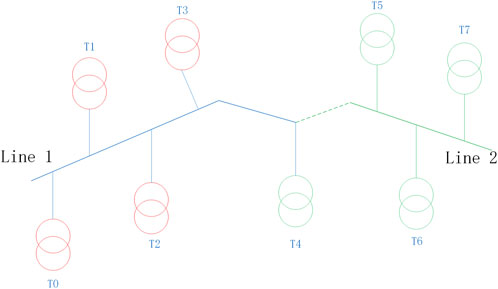
FIGURE 1. Schematic diagram of the Feeder-Transformer relationship error.

2.1 The practical problem

The distribution area plays a critical role in the final stage of transmitting electric energy to customers, highlighting its significance in the power supply chain. With the advancements in smart devices, the installation of smart meters at transformers, distribution transformers, and customer locations allows for extensive data collection on the operation of the distribution network. However, it is important to acknowledge that the collected data often suffer from inaccuracies due to various factors. Moreover, combining multiple types of data can further amplify these errors. Therefore, it becomes imperative to conduct research on utilizing a single type of data for the identification of the feeder-transformer relationship in distribution networks, aiming to address the challenges with data inaccuracies.

2.2 The feasibility of voltage data mining

In China, the distribution network is designed with a closed-loop structure and operates in an open-loop manner to ensure reliability and flexibility. This is achieved by installing numerous sectional switches, link switches, capacitor banks, and other equipment throughout the distribution network. As a result, the distribution network predominantly follows a radial configuration, where voltage drops and voltage magnitudes exhibit consistent patterns (Zhao et al., 2021). In a specific grid, as illustrated in Figure 2, Ohm’s law dictates that currents in the same phase of a circuit should be equal at all points. However, in long-distance supply lines, the inherent resistance of the line leads to losses, causing voltage drops to be higher at greater distances. Nevertheless, it is important to note that the voltage drop on the same line maintains consistency throughout its length.

FIGURE 2

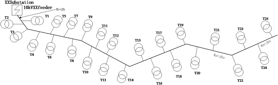
FIGURE 2. Radial Distribution Grid.

As shown in Figure 2, the voltage at node T1 in the Figure as follow:

${\mathrm{U}}_1=\mathrm{I}\left({\mathrm{R}}_1+{\mathrm{j}\mathrm{X}}_1\right)(1)$

Here I is the feeder current, R1 is the resistance in the line, and X₁ is the reactance in the line. And for the voltage at the end of the line T25 as follow:

${\mathrm{U}}_{25}=\mathrm{I}\sum \left(\mathrm{R}+\mathrm{j}\mathrm{X}\right)(2)$

Here I is the feeder current, R is the resistance in the line, and X is the reactance in the line.

Equations 1, 2 represent the principle that currents flowing through distribution transformers in the same line are equal. However, within the line, the resistance and reactance of the wire contribute to increasing values as the distance grows, resulting in a higher voltage drop at the end of the line. Simultaneously, since the resistance and reactance of the line remain constant, the voltage drop at the end of the line remains consistent. These observations provide a theoretical foundation for the utilization of voltage data in this paper for mining purposes. By analyzing the voltage measurements along the distribution network, valuable information can be extracted and utilized to identify the feeder-transformer relationship accurately.

3 Voltage dependence of feeders and distribution transformers

In this paper, a data-driven and machine-learning online identification model is proposed for the feeder-transformer relationship in distribution networks. The model is composed of two main parts: data pre-processing and correlation calculation, and the training and application of the algorithm model. This section describes the pre-processing process for the collected voltage amplitude data, including the three-phase normalization method. The formulae for calculating the correlation coefficients between stations and between stations and feeders are also presented. These steps are crucial for preparing the data and obtaining meaningful correlation measures to accurately identify the feeder-transformer relationship in the distribution network.

3.1 Data pre-processing

In practical scenarios, collected data often suffer from quality issues such as missing data, duplication, and clock desynchronization. These factors can introduce errors in the identification results. To address this, data pre-processing techniques are applied to minimize the impact of data quality issues. The pre-processing stage involves handling missing data, removing duplicates, and addressing clock desynchronization. By effectively addressing these issues, the data can be prepared for further analysis and ensure more accurate identification of the feeder-transformer relationship in the distribution network.

3.1.1 Data cleaning

In practice, there are places where multiple measurement point information exists for the same distribution transformer, and the measurement point with the most complete data retention should be selected. The specific problems that will occur and the corresponding cleaning methods are shown in Table 1.

TABLE 1

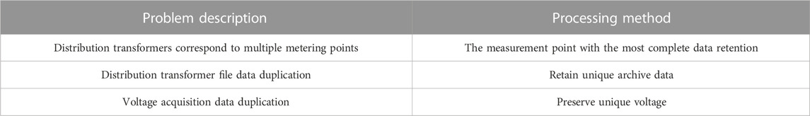
TABLE 1. Cleaning method of bad voltage data of transformer.

3.1.2 Voltage missing value detection and filling

In Figure 3, it is observed that the sampling data is prone to missing data, which can have a significant impact on the identification process. To address this issue, this paper employs two interpolation methods, namely, cubic spline interpolation and cubic polynomial interpolation, to fill in the missing data. Table 2 presents the filling effect comparison under different random missing ratios.

FIGURE 3

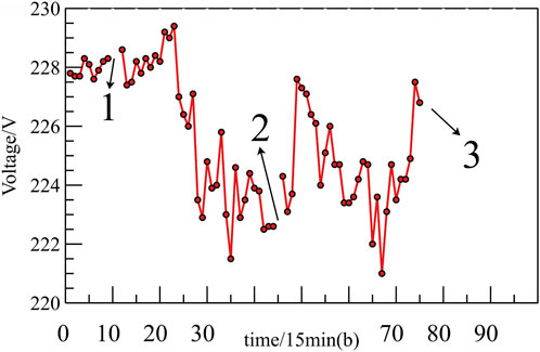
FIGURE 3. Data Loss.

TABLE 2

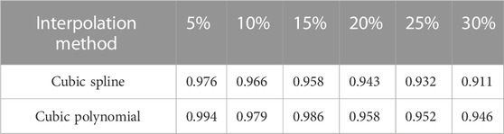
TABLE 2. Interpolated values with different data loss ratios.

The results in Table 2 demonstrate that both interpolation methods are effective in filling the missing voltage values. However, the cubic polynomial interpolation method outperforms the cubic spline interpolation method in terms of filling accuracy. The cubic polynomial interpolation achieves a higher percentage of filled data for each missing ratio. Based on this comparison, the cubic polynomial interpolation method is selected in this paper as the preferred approach for filling the missing voltage values.

By utilizing the cubic polynomial interpolation method to fill in the missing data, the issue of missing data can be effectively resolved. This ensures that the dataset used for identification of the feeder-transformer relationship is more complete and accurate. With improved data completeness and accuracy, the subsequent identification process can be conducted more reliably, leading to better results in determining the feeder-transformer relationship in the distribution network.

3.1.3 Voltage outlier detection and replacement

During the operation of the distribution network, factors such as load switching, environmental disturbances, and distribution network transient shocks can cause sudden increases or drops in the voltage collected by voltage collection equipment at the distribution outlet side. As shown in Figure 4, although this voltage data reflects the actual operation of the grid, it is considered abnormal in terms of timing data processing. Therefore, it is essential to identify and reject these abnormal values, replacing them with the average of the two adjacent voltage data points.

FIGURE 4

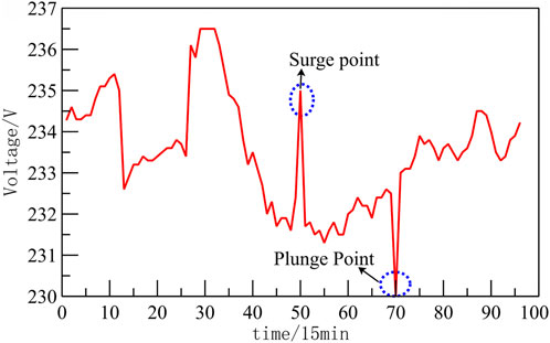
FIGURE 4. Suddenly increase (suddenly drop) of distribution transformer voltage.

3.1.4 Voltage clock offset detection

During the operation of the distribution network, discrepancies can arise in the clock calibration of measurement devices, leading to timing variations in the voltage data of distribution transformers. This can result in either an advance or a delay in the recorded voltage data. Figure 5 illustrates this situation, where the blue curve representing the voltage of transformer 2 clearly lags behind the red curve representing the voltage of transformer 1.

FIGURE 5

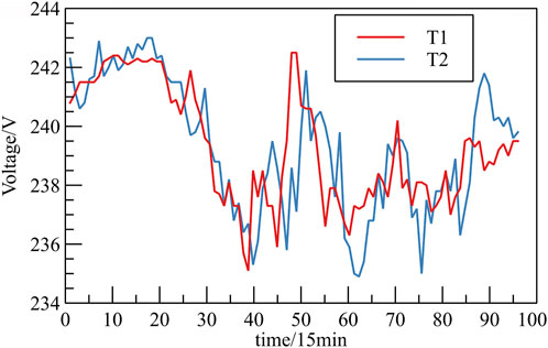
FIGURE 5. Voltage time series offset.

The Dynamic Time Warping (DTW) algorithm is a technique used to quantify the similarity between two time series. It is particularly useful for comparing time series that may have different lengths or temporal shifts. The algorithm determines the similarity by continuously adjusting the alignment between different time points of the two time series, ultimately finding the optimal path that minimizes the discrepancy between them. DTW is commonly employed when analyzing time series data to account for temporal variations and enable effective comparison and pattern recognition. Let the voltage timing data of the two distribution transformers be X(x₁,x₂,.,x_m) and Y(y₁,y₂,.,y_n), the normalization path is W(w₁,w₂,.,w_k), and the kth element w_k = (m,n)k of W.

$DTW\left(X,Y\right)=\min {\displaystyle \sum _{k-1}^K}{w}_k(3)$

Equation 3 is the DTW distance, w_k should also satisfy three constraints:

(1) The regularization path satisfies w₁ = (1,1) and w_k = (m,n);

(2) For an arbitrary 1 ≤ i < k, when w_i = (a_i,b_i),w_i+1 = (a_i+1,b_i+1), we will have a_i+1≤a_i+1 and b_i+1≤b_i+1;

(3) For an arbitrary 1 ≤ i < k, when w_i = (a_i,b_i),w_i+1 = (a_i+1,b_i+1), we will have a_i+1≥a_i,b_i+1≥b_i, and a_i + b_i ≠a_i+1+b_i+1

By applying the DTW algorithm to normalize the alignment path of the offset voltage time series, the Pearson correlation coefficient has been observed to increase from 0.77 to 0.89. This improvement in correlation signifies a stronger relationship between the time series data and indicates a reduction in the misclassification rate. The DTW algorithm effectively aligns the time series, compensating for temporal variations and enhancing the accuracy of the correlation analysis.

3.1.5 Voltage curve smoothing process

During the operation of the distribution network, various factors such as external environmental interference and clock calibration deviations can introduce deviations between the collected voltage values and the actual voltage values. Moreover, the voltage data on the outlet side of the distribution transformer often contains significant jitter noise. In Figure 6, it can be observed that the verification of the feeder-transformer relationship primarily relies on analyzing the change trend using voltage timing data. To extract this change trend, the original voltage timing data collected on the outlet side of the distribution transformer needs to undergo a smoothing process. Smoothing helps to reduce the impact of noise and highlights the underlying trend in the data.

FIGURE 6

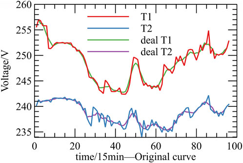
FIGURE 6. Voltage curve smoothing comparison.

In this paper, we compare the commonly used data smoothing methods include One-dimensional convolutional smoothing, Kalman filtering, Savitzky-Golay smoothing, etc. Savitzky-Golay smoothing method for voltage time series data V = [v₁,v₂,v₃,.,v₉₆] sets a sliding window W traversing the voltage timing data V with a sliding step of 1. The data for a total of 2n+1 before and after the sliding window W at moment t is W = [v_t-n,.,v_t-1,v_t,v_t+1,.,v_t+n], and the equation fitted at moment v_t as follow:

$v_t=a_0+a_{1}x+a_2{x}^2+\dots +a_{k-1}{x}^{k-1}(4)$

By substituting the sliding window W into the matrix form of the (k-1)st order polynomial equation (Eq. 4), we obtain Eq. 5.

When the number of data points in the sliding window, denoted by 2n+1, exceeds the number of parameters, k, a system of equations can be solved using the least squares method to obtain the parameters a₀,a₁,a₂, … ,a_k-1. In one scenario, when the voltage timing data in the sliding window W exhibits minimal variation, the Savitzky-Golay smoothing method is capable of effectively filtering out a significant portion of the jitter noise, resulting in a smoothing effect that closely approximates the real values. In another scenario, when the real values in the sliding window W exhibit substantial variation, the method can still filter out some of the jitter noise while preserving the local variations present in the voltage-time series data. Figure 6 illustrates the impact of voltage smoothing, where the correlation coefficient is improved as a result of the smoothing process.

$\left(\begin{array}{c}{v}_{t-n}\\ ⋮\\ v_{t-1}\\ v_t\\ v_{t+1}\\ ⋮\\ v_{t+n}\end{array}\right)=\left(\begin{array}{ccccc}1& v_{t-n}& v_{t-n}^2& \cdots & v_{t-n}^{k-1}\\ ⋮& ⋮& ⋮& ⋮& ⋮\\ 1& v_{t-1}& v_{t-1}^2& \cdots & v_{t-1}^{k-1}\\ 1& v_t& v_t^2& \cdots & v_t^{k-1}\\ 1& v_{t+1}& v_{t+1}^2& \cdots & v_{t+1}^{k-1}\\ ⋮& ⋮& ⋮& ⋮& ⋮\\ 1& v_{t+n}& v_{t+n}^2& \cdots & v_{t+n}^{k-1}\end{array}\right)\left(\begin{array}{c}{a}_0\\ a_1\\ a_2\\ ⋮\\ a_{k-1}\end{array}\right)+\left(\begin{array}{c}{\epsilon }_{t-n}\\ ⋮\\ {\epsilon }_{t-1}\\ {\epsilon }_t\\ {\epsilon }_{t+1}\\ ⋮\\ {\epsilon }_{t+n}\end{array}\right)(5)$

3.2 Unbalanced three-phase voltage processing

The power consumption information collection system gathers the timing data of three-phase voltage from the distribution transformer. Typically, either a single-phase voltage is selected from the three-phase voltage or the three-phase voltage is converted into a single-phase voltage to facilitate similarity calculation during the verification of the feeder-transformer relationship.

In practical scenarios, distribution transformers with the Dyn11 wiring method typically exhibit balanced outlet three-phase voltages. In such cases, the average value of the three-phase voltage timing data can be utilized as a representative single-phase voltage. On the other hand, distribution transformers with the Yyn0 wiring method have an ungrounded neutral point on the high-voltage side. When the three-phase load is unbalanced, it causes a shift in the neutral point. In public transformer station areas, most users receive power from a single phase of the distribution transformer, resulting in an unbalanced three-phase voltage at the transformer’s outlet due to the unequal load carried by each phase. This unbalance poses a significant challenge to the identification of the feeder-transformer relationship. To address this issue, it becomes necessary to estimate the unbalanced three-phase voltage. The first step is to calculate the degree of unbalance for the collected voltage data, as shown in Eq. 6.

$P_V=\frac{\max \left[\left|V_a-V_{Pavg}\right|,\left|V_b-V_{Pavg}\right|,\left|V_c-V_{Pavg}\right|\right]}{V_{Pavg}}\times 100\%(6)$

In formula (6), Va, Vb, Vc are the three phase voltages of ABC on the exit side of the distribution transformer, and V_Pavg is the average value of the three phase voltages. When the percentage of values in the P_V solution exceeds 95% as defined by the current standards, the unbalanced voltages in three phases need to be recalculated to their balanced state using an iterative approach for each moment’s phase voltage. Figure 7 illustrates a schematic diagram of neutral point displacement at the high-voltage side of the transformer.

FIGURE 7

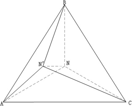
FIGURE 7. Distribution transformer high-voltage side neutral point offset figure.

In Figure 7, AN, BN, and CN represent the three-phase voltage when the three-phase load is balanced, while AN’, BN’, and CN’ represent the three-phase voltage when the three-phase load is unbalanced. In the Figure, triangle ABC is an equilateral triangle, AB, AC, BC is the line voltage, in the normal case, AN = BN = CN = X. From trigonometric functions, we can know AB² = AC² = BC² = 3X². Based on the cosine theorem, the following format can be derived (Tang et al., 2018):

$\cos \angle B{N}^{\prime }A=\frac{A{N}^{\prime 2}+B{N}^{\prime 2}-A{B}^2}{2\times A{N}^{\prime }\times B{N}^{\prime }}(7)$

$\cos \angle B{N}^{\prime }C=\frac{B{N}^{{\prime }^2}+C{N}^{{\prime }^2}-B{C}^2}{2\times B{N}^{\prime }\times C{N}^{\prime }}(8)$

$\cos \angle A{N}^{\prime }C=\frac{A{N}^{{\prime }^2}+C{N}^{\prime 2}-A{C}^2}{2\times A{N}^{\prime }\times C{N}^{\prime }}(9)$

$\angle B{N}^{\prime }A+\angle B{N}^{\prime }C+\angle A{N}^{\prime }C=2\pi (10)$

Combining Eqs 7–10 yields Eq. 11.

$\mathrm{a}\mathrm{r}\mathrm{c}\cos \frac{A{N}^{{\prime }^2}+B{N}^{{\prime }^2}-A{B}^2}{2\times A{N}^{\prime }\times B{N}^{\prime }}+\mathrm{a}\mathrm{r}\mathrm{c}\cos \frac{B{N}^{{\prime }^2}+C{N}^{{\prime }^2}-B{C}^2}{2\times B{N}^{\prime }\times C{N}^{\prime }}+\mathrm{a}\mathrm{r}\mathrm{c}\cos \frac{A{N}^{{\prime }^2}+C{N}^{{\prime }^2}-A{C}^2}{2\times A{N}^{\prime }\times C{N}^{\prime }}=2\pi (11)$

In the above equation, AN’, BN’, CN’ are already known, only X is unknown. According to the specification, the voltage qualification range of the distribution is between +7% and −10% of 220 V, so the solution interval of X is set to [190, 250], and the solution accuracy is 0.1, and X can be found using the iterative method. Further, AN, BN, and CN can be calculated, and the values obtained are the data after the balancing process. Then, the same phase data of any different transformer can be selected for the next step of similarity calculation.

3.3 Voltage correlation

Correlation analysis of time series is a commonly used method in the field of time series data mining. In the context of distribution networks, voltage fluctuations often occur due to uncertainties in the load at different locations along the line. As depicted in Figure 8, the fluctuation patterns of voltage curves belonging to the same phase in different distribution transformers under the same line exhibit a noticeable consistency. Conversely, the fluctuation patterns of voltage curves under two different lines display distinct differences. Therefore, the consistency of voltage fluctuation trends on the outlet side between distribution transformers can serve as a significant feature for identifying the feeder-transformer relationship. The correlation calculation proposed in this paper involves determining the correlation between distribution transformers and the correlation between distribution transformers and the line.

FIGURE 8

FIGURE 8. Different distribution transformer voltage curves under the same line.

The correlation between distribution transformers refers to the relationship between any two transformers that are located on the same line. In Chapter 3, Section 2, after the data processing described, we can select different transformer data from the same phase and perform correlation calculations. This allows us to assess the degree of similarity or consistency between the voltage data of different transformers, providing valuable insights into the feeder-transformer relationship.

In general, the Euclidean distance is commonly used to measure the correlation between two time series. A smaller Euclidean distance indicates a higher correlation, while a larger Euclidean distance suggests a lower correlation. However, since different time series may have varying magnitudes, it is often necessary to scale the data to a common magnitude before using the Euclidean distance for comparison. Although the Euclidean distance is widely used, it can be sensitive to abnormalities, noise, and temporal deformations present in the measured data, leading to unstable calculation results. To address this issue, it is beneficial to utilize a dimensionless measure of correlation between two time series. This alternative approach helps mitigate the problem caused by the Euclidean distance, resulting in more stable and reliable calculation outcomes.

Pearson’s correlation coefficient, also known as Pearson’s product-moment correlation coefficient, is used to measure the degree of linear correlation between two independent variables and is calculated as:

${\rho }_{X,Y}=\frac{\mathrm{c}\mathrm{o}\mathrm{v}\left(X,Y\right)}{{\sigma }_X{\sigma }_Y}=\frac{n{\displaystyle \sum _{i=1}^n}{x}_i{y}_i-{\displaystyle \sum _{i=1}^n}{x}_i{\displaystyle \sum _{i=1}^n}{y}_i}{\sqrt{n{\displaystyle \sum _{i=1}^n}{x}_i^2-{\left({\displaystyle \sum _{i=1}^n}{x}_i\right)}^2}\sqrt{n{\displaystyle \sum _{i=1}^n}{y}_i^2-{\left({\displaystyle \sum _{i=1}^n}{y}_i\right)}^2}}(12)$

In Eq. 12, cov(X,Y) is the covariance of the ligand X and the ligand Y. σx, σy are the standard deviations of the ligand X and the ligand Y, respectively.

From Eq. 12, the correlation coefficient between distribution transformer under the same line can be calculated. By applying the Pearson correlation coefficient calculation to the time series of distribution transformer voltage for the same line, a distribution transformer correlation matrix can be obtained. This matrix represents the correlation coefficients between different distribution transformer and can be expressed as follows:

$P=\left[\begin{array}{ccccc}1& {\rho }_{\mathrm{1,2}}& \cdots & {\rho }_{1,n-1}& {\rho }_{1,n}\\ {\rho }_{\mathrm{2,1}}& 1& \cdots & {\rho }_{2,n-1}& {\rho }_{2,n}\\ ⋮& ⋮& \ddots & ⋮& ⋮\\ {\rho }_{n-\mathrm{1,1}}& {\rho }_{n-\mathrm{1,2}}& \cdots & 1& {\rho }_{n-1,n}\\ {\rho }_{n,1}& {\rho }_{n,2}& \cdots & {\rho }_{n,n-1}& 1\end{array}\right](13)$

In this correlation matrix, the main diagonal represents the distribution transformer themselves, and their Pearson correlation coefficients are constant with a value of 1. The remaining positions in the matrix represent the Pearson correlation coefficients between the distribution transformer voltage time series of two distribution transformer. These coefficients are symmetric about the main diagonal, indicating the correlation between different pairs of distribution transformer. The size of the correlation matrix is determined by the number of distribution transformer under the line, denoted as “n”.

The same formula (12) is used for the calculation of the correlation coefficient between the distribution transformer and the line. cov(X,Y) is the covariance of the ligand X and the ligand Y. σx, σy are the standard deviations of the ligand X and the ligand Y, respectively.

The correlation coefficient between the line and the distribution transformer calculated by Eq. 12 also yields the correlation matrix:

$P_X=\left[{\rho }_1,{\rho }_2,\cdots {\rho }_n\right](14)$

Each element of this correlation matrix represents the correlation coefficient of a distribution transformer and the line.

4 DDML algorithm

In this subsection, we present the distribution network line-variation relationship identification algorithm that combines data-driven approaches with machine learning. The focus is on introducing the proposed random forest algorithm and selecting the optimal feature construction matrix for model training. The random forest algorithm is utilized as the underlying machine learning method in this study. It is a powerful ensemble learning technique that combines multiple decision trees to make accurate predictions. By leveraging the random forest algorithm, we aim to achieve robust and reliable identification of the line-variation relationships in the distribution network.

To train the random forest model effectively, the construction of the feature matrix plays a crucial role. Various features are extracted from the collected data to represent the characteristics of the distribution network. The selection of the optimal feature construction matrix is a key step in enhancing the performance of the model.

By carefully selecting and constructing the feature matrix, we can capture the essential information and patterns in the data, allowing the random forest algorithm to make accurate predictions for line-variation relationship identification in the distribution network.

4.1 Random forest algorithm

The random forest algorithm is an ensemble learning method that combines multiple decision trees to make predictions. It is based on the idea of Bagging, which involves training each decision tree on a random sample of the overall dataset. The model parameters are determined by aggregating the predictions of individual decision trees, such as through voting or averaging.

By integrating multiple machine learning models, the random forest algorithm offers several advantages over using a single learner. It tends to achieve higher accuracy, as the combination of multiple models helps to reduce bias and variance. It is also less prone to overfitting, as the averaging or voting process helps to generalize the predictions. Additionally, the random forest algorithm exhibits strong resilience to interference, making it robust in handling noisy or inconsistent data.

The decision tree serves as the base learner in the random forest algorithm. Figure 9 illustrates the construction process of a decision tree. Initially, different decision trees are constructed by partitioning the dataset using different subsets of the data. Each decision tree undergoes node splitting and randomly selects feature variables for the split. Finally, the random forest model is built from multiple decision trees, and the final classification result of a sample is determined by aggregating the predictions through a voting mechanism.

FIGURE 9

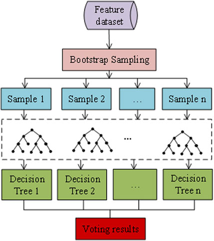
FIGURE 9. Random forest algorithm construction.

Overall, the random forest algorithm combines the strengths of individual decision trees to create a powerful and reliable model for classification and prediction tasks.

4.2 Feature selection and construction

To enhance the generalization ability of the machine learning model, it is necessary to construct meaningful features from the voltage time series data of distribution transformers. Instead of directly inputting the high-dimensional parameter of the voltage time series, a set of eight features are selected in this paper to capture different aspects of the time-series characteristics. These features are chosen to provide a comprehensive representation of the voltage time series.

By considering these eight features, the model can learn not only the instantaneous characteristics of the voltage time series but also the statistical properties and patterns within the series. This feature construction approach enables the model to generalize well to voltage time series data from different dates and enhances its ability to capture the underlying patterns and trends in the distribution transformer voltage.

(1) Skewness

The skewness indicator reflects the asymmetry of the time-series data distribution and its calculated equation is as follows:

$x_{sk}=E\left[{\left(\frac{V^{\prime }-\mu }{\sigma }\right)}^3\right](15)$

(2) Kurtosis

The kurtosis indicator reflects the steepness of the voltage-time series data distribution and is calculated as follows:

$x_{ku}=E\left[{\left(\frac{V^{\prime }-\mu }{\sigma }\right)}^4\right](16)$

(3) Discrete values

The dispersion coefficient is a relative statistic that measures the degree of dispersion of the data and is mainly used to compare the degree of dispersion of different sample data. It is denoted as xs.

(4) Number of line distribution transformers

This indicator directly reflects the topological complexity of the line and the diversity of load changes and it is an important indicator that affects the calibration of the feeder-transformer relationship, denoted as xn.

(5) Percentage of dedicated transformers

The quality of the voltage data of dedicated transformers varies, and this indicator is also an important indicator affecting the calibration of the feeder-transformer relationship, denoted as xz.

(6) Distribution transformer correlation

Calculating the correlation between different distribution variables yields Eq. 13, and then take the mean value of each column to obtain ${\rho }_t=\left[{\rho }_1,{\rho }_2,\cdots {\rho }_n\right]$, denoted as $X_{\rho }$.

(7) Mean value of line distribution transformer correlation

Take Eq. 14 derived from the value to xl, the indicator reflects the degree of correlation between the line and the distribution transformer, denoted as xl.

(8) Distribution transformer sliding window correlation

The Pearson correlation coefficient provides a measure of the overall correlation between distribution transformer voltage time series. However, in real-world operation, various factors such as load imbalances and transformer tap shifting can introduce offsets in the voltage time series data, affecting the accuracy of the global Pearson correlation coefficient calculation. In some cases, the global Pearson correlation coefficient may be low, but there may still be a high correlation between the voltage time series of specific distribution transformers within a sliding window.

To address this, a sliding window approach is adopted to calculate the Pearson correlation coefficients between distribution transformer voltage time series within the window. The average value of these window correlation coefficients (xw) is considered as a new feature, which is added to the feature vector. This approach aims to improve the accuracy of feeder-transformer relationship calibration and reduce misclassification rates.

In the end, the eight selected features, including statistical indicators, discrete values, and correlation coefficients, are constructed as a feature matrix according to Eq. 17. This feature matrix is used as input for offline training of the random forest model. After the training is completed and optimal parameters are selected, the model can be applied for the identification of feeder-transformer relationships.

$\left[\begin{array}{cccccccc}{x}_{sk,1}& x_{ku,1}& x_{s,1}& x_{n,1}& x_{z,1}& x_{\rho ,1}& x_{l,1}& x_{w,1}\\ x_{sk,2}& x_{ku,2}& x_{s,2}& x_{n,2}& x_{z,2}& x_{\rho ,2}& x_{l,,2}& x_{w,2}\\ ⋮& ⋮& ⋮& ⋮& ⋮& ⋮& ⋮& ⋮\\ x_{sk,i}& x_{ku,i}& x_{s,i}& x_{n,i}& x_{z,3}& x_{\rho ,i}& x_{l,i}& x_{w,i}\end{array}\right](17)$

4.3 Model training

The experimental environment for this paper is Windows 10 with the following configuration: Intel(R) Xeon(R) Gold 5120T CPU @ 2.20 GHz 2.19 GHz Graphics card is NVIDIA-P5000.

In this method, the preprocessing and feature construction of the distribution transformer voltage time series data are performed using the Pandas and NumPy libraries in the Python environment. These libraries provide useful functions for data manipulation and feature extraction.

Once the feature dataset is prepared, the next step is to construct and train the random forest model. The random forest algorithm is implemented using libraries such as Scikit-Learn (SKLearn) in Python.

To evaluate the performance of the trained model and assess its generalization ability, the feature dataset is split into a training set and a test set. The train_test_split function from the SKLearn library is used for this purpose. Typically, the training set contains 70% of the data, while the remaining 30% is allocated to the test set. This partitioning allows for cross-validation, which helps in assessing the model’s performance on unseen data.

To ensure reliable evaluation, cross-validation is performed using 10-fold cross-validation. This means that the dataset is divided into 10 equal parts, and the model is trained and evaluated 10 times, each time using a different fold as the test set while the remaining folds are used as the training set. This approach provides a more robust assessment of the model’s performance by considering different combinations of training and test data.

By following this process, the distribution transformer voltage time series data is preprocessed, features are constructed, and a random forest model is trained and evaluated using cross-validation techniques to ensure accurate and reliable results.

The modeling of the classified random forest using the scikit-learn library Random forest consists of numerous decision trees, so the number of decision trees has the greatest impact on the complexity of the random forest model. The parameter n_estimators is set in the interval [1–200] with a step size of 10 to observe the trend of the change in the number of decision trees on the classification accuracy of the model, a diagram of the specific training process as shown in Supplementary Figure S1.

As can be seen in Supplementary Figure S1, the F1-score of the model is highest at 0.84 when n_estimators is taken to be around 50, and then the F1-score of the model shows an oscillating and slightly decreasing trend as n_estimators increases. Since the step size of n_estimators is 10, it is easy to miss the optimal F1-score within the step size. To determine the optimal value of n_estimators, Supplementary Figure S1 between 40–70 with a step size of 1 is taken for secondary learning and cross-validation to obtain the F1-score curve, a diagram of the specific training process as shown in Supplementary Figure S2. From the quadratic learning F1-score curve, it can be seen that the classification performance of the model is optimal at 0.8432 when n_estimators is taken as 45. Compared with the value of 50 when n_estimators is only improved by 0.0032, it shows that adjusting this parameter can no longer improve the classification performance of the model, so the optimal value of n_estimators is selected as 45.

The decision tree splitting algorithm has two types based on information entropy and Gini coefficient, so the model training is set 20 times with the same model parameters to obtain the F1-score curve as shown in Supplementary Figures S3A, B. The overall F1-score fluctuates around 0.84 as can be seen from Supplementary Figure S3. But the Gini coefficient fluctuates more smoothly. Criterion parameter is chosen as the Gini coefficient.

The maximum depth parameter of the max_depth decision tree is generally chosen according to the number of data features. When the maximum depth of the decision tree is increased, the decision tree will capture more useful information in the data, but it will also increase the risk of overfitting the random forest. When the maximum depth is set too small, the flexibility of the decision tree is reduced and underfitting is easily produced. For the voltage time series data in this paper, the max_depth is set in the range of [1–30] with a step size of 1 to obtain the F1-score curve, as shown in Supplementary Figure S4.

It can be seen from Supplementary Figure S4. That the classification performance of the random forest model reaches the optimum when the max_depth takes the value of 21, with F1-score of 0.8824. And then the F1-score value remains unchanged as the depth of the tree grows, and the F1-score value grows by 0.0392 compared to 0.8432, at which time the model lies to the right of the lowest point of generalization error.

To reduce the complexity of the random forest model and obtain a smaller generalization error, it needs to further learn and choose the appropriate parameter values of min_samples_split and min_samples_leaf. The parameter values in scikit-learn are integers larger than 2, sot the parameter value interval should be set as [2–30] and the step size as 1 to obtain the F1-score scoring curve.

From Supplementary Figure S5, it is known that the highest level of random forest model F1-score is 0.8947 when min_samples_split is 12. From Supplementary Figure S6, it can be seen that the highest level of random forest model F1-score is 0.9186 when min_samples_leaf is 10.

By analyzing the learning curve of the parameters, it can be seen that the generalization error of the random forest model keeps decreasing, so it needs to further try to adjust the max_features parameter to further reduce the complexity of the model and observe whether the generalization error of the model still has room to decrease. Set the max_features parameter interval to [1–9] with a step size of 1. The F1-scoring curve is obtained as shown in Supplementary Figure S7. From Supplementary Figure S7, it can be seen that the optimal value of the F1-score for the random forest model reaches 0.9209 when the max_features parameter is set to 5. Compared to 0.9186, the F1-score value only increases by 0.0023, and the generalization error of the model is very close to the lowest point.

The optimal values of each parameter of the final random forest-based feeder-transformer relationship calibration model are shown in Table 3.

TABLE 3

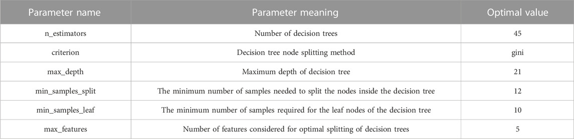
TABLE 3. Optimal parameter values for the random forest model.

4.4 Algorithm processing sequence

After detailing the necessary data processing steps and outlining the essential calculations, this subsection presents the specific algorithm flow. The proposed method solely relies on the voltage data collected by the production management system (PMS) in the Chinese distribution network. The formal description of the algorithm is provided in Table 4.

TABLE 4

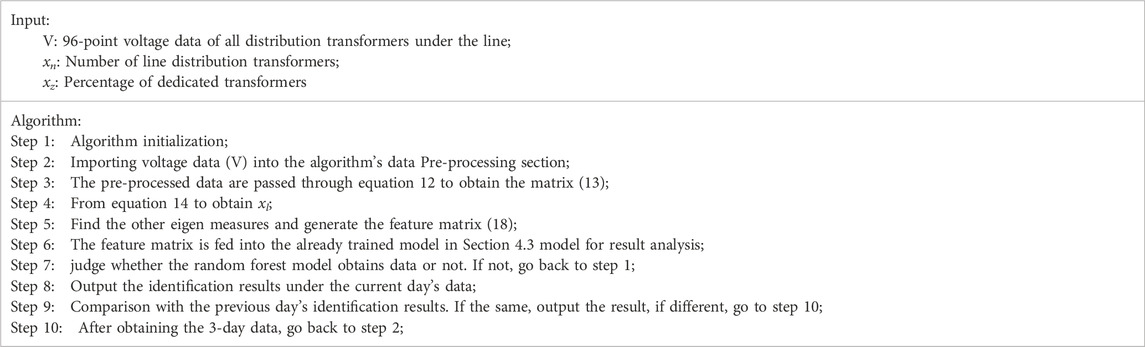
TABLE 4. Feeder-transformer relationship recognition algorithm.

One crucial aspect of the algorithm is its ability to operate in real-time. Therefore, it should be executed periodically whenever the PMS acquires new data to determine the current feeder-transformer relationship. Setting the execution interval requires careful consideration to strike a balance. If the interval is too short, the algorithm may yield a low correlation coefficient for the voltage time series, leading to incorrect identification. On the other hand, if the interval is too long, a large amount of data will accumulate, resulting in longer computation times and wastage of computational resources. Hence, a comprehensive approach is needed to determine the most appropriate implementation cycle.

For instance, in China, voltage data is collected every 15 min, resulting in 96 data points per day. At the end of each day, the collected data for that day is frozen, and the data collection for the next day begins. Therefore, each day’s data can be utilized to identify the feeder-transformer relationship. The program will output the result if it detects any inconsistencies with the previous day’s result after execution.

Once the daily data is frozen, the feeder-transformer relationship in the distribution network is identified using the voltage data collected on that day. Before initiating the identification process, the entire algorithm needs to be initialized. In Step 2, the voltage data (V) for the current day is imported and passed through the data pre-processing component of the algorithm. This involves applying the data pre-processing algorithm described in Chapter 3, Section 1 to process the data and calculate the extraction of feature values. Subsequently, the trained model is used to generate the feature matrix, which is then utilized for identification. Prior to this step, it is verified whether there is any input data for the feature matrix. If no data is available, the algorithm returns to Step 1 to restart the process.

The output results are compared with the previous results. If inconsistencies are detected, a 3-day data set is extracted and sent back to Step 2 for joint calculation.

5 Case studies

This section presents the computational results obtained from the proposed algorithm and compares them with the results of other algorithms. The analysis focuses on evaluating the performance and effectiveness of the proposed algorithm in relation to alternative approaches.

5.1 Dataset

In order to validate the effectiveness of the proposed algorithm, a 0.4 kV distribution network located in Jiangxi Province was selected as the test network. This particular distribution network consists of three substations and 18 feeders, representing a typical scenario with long-distance supply lines and short-distance complex lines. The selected feeders contain both single-phase power from residential users and three-phase power from industrial users. This variety of power supply configurations reflects the complexity of real-world distribution networks in China.

The test cases included in the study cover a mix of dedicated and public transformers within the distribution network. By incorporating the data from distribution transformers in a city, a comprehensive evaluation of the algorithm’s performance was conducted. It is worth noting that all the identification results obtained through the algorithm were verified on-site by experienced engineers, ensuring the accuracy and reliability of the findings.

While existing test networks such as IEEE-33 nodes and IEEE-69 nodes are commonly used for power system-related algorithm testing, they are not directly applicable to the unique characteristics of the Chinese distribution network. The selection of a representative distribution network in Jiangxi Province provides a more realistic and practical basis for evaluating the algorithm’s performance in the context of the Chinese distribution network.

By conducting the analysis on the actual distribution network and verifying the results on-site, the proposed algorithm’s capability to identify the feeder-transformer relationship in a real-world setting is thoroughly examined.

5.2 Analysis of practical application results

5.2.1 Long distance lines

In the first scenario, the focus was on the SQ 10 kV long-distance power supply line and the SL line that runs along the country road, providing electricity to villages and dedicated users along the way. Voltage data from all distribution transformers under the SQ line on 16 August 2021, were processed and used to extract feature quantities. These features were then fed into the trained model for feeder-transformer relationship identification.

The extracted features are presented in Tables 5, 6, and the model’s output results are shown. Figure 10 depicts the recorded feeder topology of the SQ line as captured by the GIS system. The analysis of the results revealed an error in the feeder-transformer relationship for distribution transformers T25 and T26, which are two adjacent utility transformers.

TABLE 5

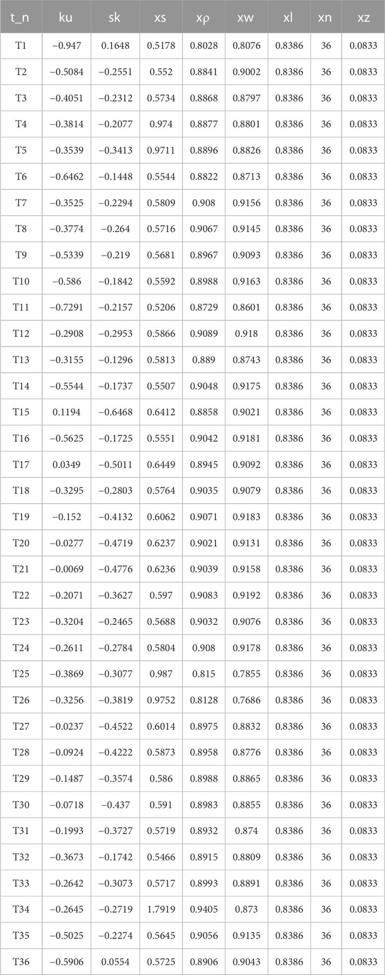
TABLE 5. Scenario 4 line Eigenvalue.

TABLE 6

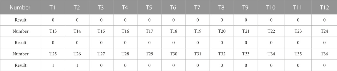
TABLE 6. Scenario 4 line results.

FIGURE 10

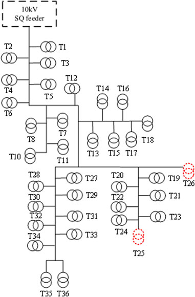
FIGURE 10. SQ feeder topology figure.

Further examination of the data revealed that the characteristic data of the two transformers in error were similar. However, their correlation coefficient with other distribution transformers was unusually low, as shown in Table 5. To verify the accuracy of the results, field staff conducted an inspection using visual examination and distribution transformer identifier analysis. The results confirmed that T25 and T26 indeed had a misidentified line relationship, validating the model’s successful identification of the incorrect distribution transformers.

Upon conducting an in-depth analysis, it was discovered that the two misidentified distribution transformers were located at the very end of the line. In the specific SQ feeder, transformers were predominantly centrally positioned at the first end, primarily serving factories and enterprises with high electricity loads and irregular consumption patterns. These users exhibited significant differences in electricity consumption behavior compared to users connected to public transformers. Additionally, the end position of the long-distance line itself experienced higher voltage drop, resulting in poorer voltage waveforms at T25 and T26 compared to other distribution transformers on the line. Despite these challenges, the random forest model successfully identified the errors in the feeder-transformer relationship.

Finally, after consulting the equipment maintenance, additions, and cancellations records, it was confirmed that the two distribution transformers had indeed been removed due to user cancellations. However, the meters associated with those transformers were relocated to another adjacent feeder originating from the same substation.

5.2.2 Short distance lines

The second scenario involves the SL 10 kV short-distance lines, which are situated in an area that recently underwent a pilot area renovation to enhance power supply reliability. This particular distribution network area exhibits a higher level of complexity. The SL feeder, spanning a distance of 4.5 km, consists of a combination of cable and overhead lines, and encompasses 26 distribution transformers, including 3 dedicated transformers and 23 public transformers. Figure 11 displays the topology of the SL feeder as stored in the GIS system. The feeder incorporates various equipment such as ring cabinets, circuit breakers, and cable branch boxes.

FIGURE 11

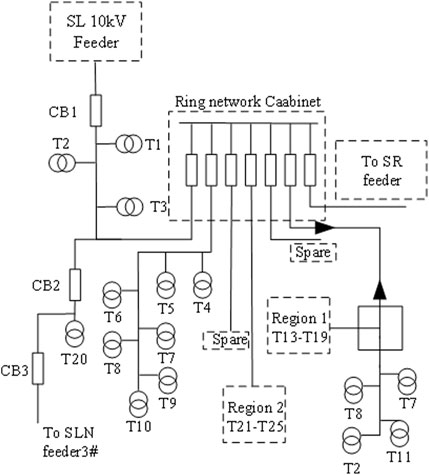
FIGURE 11. SL feeder topology figure.

For analysis purposes, the same 96 points of voltage data from all distribution transformers along the SL line on 16 August 2021, were selected and processed. Table 7 presents the processed feature data, while Table 8 showcases the calibration results obtained from the random forest model. It is noteworthy that despite the line traversing multiple intelligent devices and exhibiting high complexity, only one distribution transformer was found to have an incorrect feeder-transformer relationship.

TABLE 7

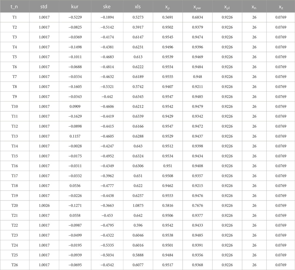
TABLE 7. Scenario 5 line Eigenvalue.

TABLE 8

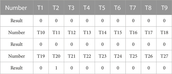
TABLE 8. Scenario 5 line results.

Through a comparative analysis, it was determined that the utility transformer T20 was the one with the erroneous relationship. Upon examining its topology diagram, it was observed that circuit breakers were present at both ends of the branch where the utility transformer was installed. When the circuit breakers were operated in reverse, the line associated with the utility transformer also switched accordingly. This ultimately resulted in the incorrect feeder-transformer relationship, a finding that was corroborated by the on-site inspection conducted by the staff.

5.2.3 All distribution network transformers in a city

To validate the effectiveness of the proposed method on a larger scale and facilitate its practical implementation, a 3-day dataset was utilized to verify the feeder-transformer relationships. The dataset consisted of data collected from a provincial municipal company from August 15 to 17 August 2021. It encompassed distribution network ledger data, distribution transformer outlet voltage data obtained from the electricity consumption information collection system, and distribution network GIS information. The dataset comprised a total of 23,838 distribution transformers under 535 10 kV feeders in the local municipality, along with the corresponding topology diagram for verification.

Construct the feature matrix according to Section 4.2, the matrix was input into the trained random forest model for direct verification. The model output identified 486 distribution transformers with incorrect feeder-transformer relationships. Subsequently, a comparison was conducted between the distribution transformers flagged by the model and the corresponding topology diagram. The verification process involved sending the list of identified transformers to each grid company for on-site verification, and the results are presented in Table 9.

TABLE 9

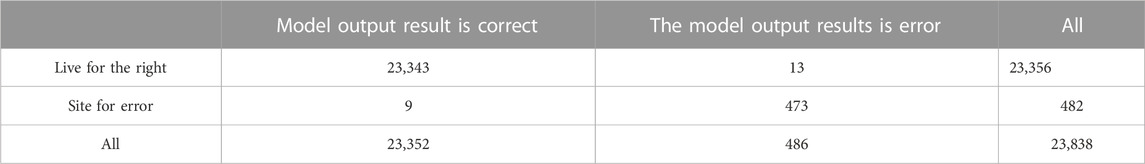
TABLE 9. Feeder and transformers check result.

From the data in Table 9, the overall accuracy of the calibration results (Accuracy) can be calculated to be 99.96%. The proportion of mismatched matches among the distribution transformers is negligible. Even if the model were to classify all mating changes as correct without any discrimination, the accuracy would still reach 97.92%. Therefore, accuracy alone does not fully reflect the actual effectiveness of the model calibration. To assess the model’s performance in identifying mismatched matches, precision and recall of the model output were computed. Using the formulas for binary problems, the precision was found to be 96.30%, the recall was 97.33%, and the F1-score was 97.73%.

5.2.4 Comparison of methods

To assess the effectiveness of the proposed method, a comparison was conducted with other common classification algorithms in order to verify its performance. The selected algorithms for comparison included Support Vector Machine, K-Nearest Neighbor, Parsimonious Bayes, and AdaBoost. The comparison experiments focused on the identification of both correct and incorrect feeder-transformer relationships.

Table 10 presents the results of identifying the correct feeder-transformer relationships, while Table 11 displays the results of identifying the incorrect feeder-transformer relationships. In Table 11, it is evident that the random forest algorithm outperformed the other classification models in terms of F1-score, accuracy, and completeness rates for both correct and incorrect feeder-transformer relationships. These results indicate the superiority of the random forest algorithm in effectively identifying feeder-transformer relationships compared to other commonly used classification algorithms.

TABLE 10

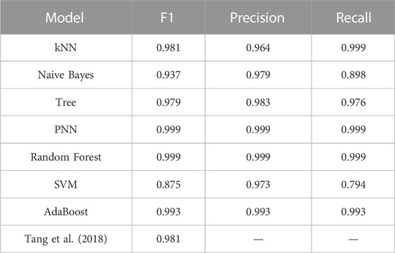
TABLE 10. Correct transformers check results of feeder transformers relationship.

TABLE 11

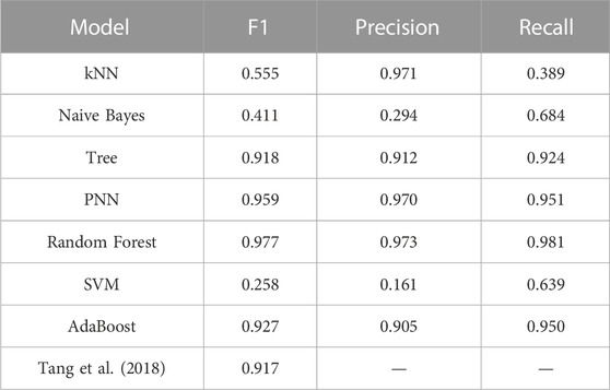
TABLE 11. Wrong transformers check results of feeder transformers relationship.

6 Conclusion

The proposed algorithm in this paper offers a data-driven and machine learning approach for identifying the feeder-transformer relationship in distribution networks. Unlike existing methods, this approach does not require additional hardware equipment but instead leverages data mining techniques and machine learning algorithms. By extracting voltage amplitude data and performing feature extraction and construction, a model is trained to effectively identify the feeder-transformer relationship. The algorithm’s performance was evaluated using real measured data, leading to the following conclusions:

1) The algorithm proposed in this paper exhibits a high level of robustness in handling collected data, effectively dealing with measurement errors and other uncertainties.

2) The method presented in this paper addresses the limitations of single-feature approaches in data-driven methods by utilizing multiple feature quantities to construct a comprehensive feature matrix. This approach significantly reduces the false alarm rate.

3) By employing machine learning techniques, the proposed algorithm leverages the constructed feature matrix for accurate and reliable feeder-transformer relationship recognition. This approach overcomes the challenges associated with determining correlation coefficient identification thresholds in existing methods.

4) The proposed method is practical and readily applicable, as the trained model demonstrates strong generalization capabilities. Once trained, it can be deployed for real-world applications.

5) This paper introduces a relevant imputation method specifically designed to address the issue of three-phase voltage unbalance in distribution transformers. This method effectively improves the correlation coefficient in cases of unbalanced three-phase voltages, contributing to the overall accuracy and reliability of the algorithm.

These findings highlight the effectiveness and practical applicability of the proposed algorithm in addressing the challenges associated with feeder-transformer relationship identification in distribution networks. By providing accurate and timely insights into the network topology and line-to-variable relationship, this algorithm can greatly enhance the operation and management of power grid companies.

In future work, we plan to extend our research to explore the identification of line-to-variable relationships in distribution networks under various disturbances. Our focus will be on addressing the challenges posed by the bi-directional flow of tidal currents caused by the increased penetration of distributed energy sources, because when a large number of distributed photovoltaic power generation and other access will lead to the phenomenon of backward transmission of electricity, further exacerbating the difficulty of identifying the topology of the distribution network. Specifically, we aim to investigate the accurate identification of distribution network topology in the presence of these dynamic conditions. This research will contribute to the development of more comprehensive and robust methods for managing distribution networks with high levels of distributed energy source integration.

Data availability statement

The raw data supporting the conclusion of this article will be made available by the authors, without undue reservation.

Author contributions

YG: conceptualization, methodology, software, validation, writing—original draft. BK: supervision, writing—review and editing, funding acquisition. HX: methodology, visualization, and investigation. ZW: software and validation. GD: writing—review and editing. ZX: methodology. CL: data curation. DW and YL: translation and retouching. All authors contributed to the article and approved the submitted version.

Conflict of interest

The authors declare that the research was conducted in the absence of any commercial or financial relationships that could be construed as a potential conflict of interest.

Publisher’s note

All claims expressed in this article are solely those of the authors and do not necessarily represent those of their affiliated organizations, or those of the publisher, the editors and the reviewers. Any product that may be evaluated in this article, or claim that may be made by its manufacturer, is not guaranteed or endorsed by the publisher.

Supplementary material

The Supplementary Material for this article can be found online at: https://www.frontiersin.org/articles/10.3389/fenrg.2023.1225407/full#supplementary-material

References

Alam, S., Natarajan, B., and Pahwa, A. (2014). Distribution grid state estimation from compressed measurements. IEEE Trans. Smart Grid 5 (4), 1631–1642. doi:10.1109/TSG.2013.2296534

CrossRef Full Text | Google Scholar

Badawi, M., Ibrahim, S., Mansour, D., El-Faraskoury, A., Ward, S., Mahmoud, K., et al. (2022). Reliable estimation for Health index of transformer oil based on novel combined predictive maintenance techniques. IEEE Access 10, 25954–25972. doi:10.1109/access.2022.3156102

CrossRef Full Text | Google Scholar

Byun, H., Zheng, Y., Choi, S., and Shon, S. (2018). New identification method for power transformer and phase in distribution systems. Appl. Mech. Mater 878, 291–295. doi:10.4028/www.scientific.net/AMM.878.291

CrossRef Full Text | Google Scholar

Cavraro, G., and Kekatos, V. (2019). Inverter probing for power distribution network topology processing. IEEE Trans. Control Netw. Syst. 6 (30), 980–992. doi:10.1109/TCNS.2019.2901714

CrossRef Full Text | Google Scholar

Cavraro, G., Kekatos, V., and Veeramachaneni, S. (2019). Voltage analytics for power distribution network topology verification. IEEE Trans. Smart Grid 10 (1), 1058–1067. doi:10.1109/TSG.2017.2758600

CrossRef Full Text | Google Scholar

Darwish, M., Hassan, M., Nagat, A., and Diaa-Eldin, M. (2022a). “A new method for estimating transformer Health index based on ultraviolet-visible spectroscopy,” in 2022 23rd International Middle East Power Systems Conference (MEPCON), Cairo, Egypt, 13 Dec 2022, 15 Dec 2022 (IEEE).

CrossRef Full Text | Google Scholar

Darwish, M., Hassan, M., Nagat, A., and Diaa-Eldin, M. (2022b). “Application of infrared spectroscopy for discrimination between electrical and thermal faults in transformer oil,” in 2022 9th International Conference on Condition Monitoring and Diagnosis (CMD), Kitakyushu, Japan, 13-18 November 2022 (IEEE), 255–258. doi:10.23919/CMD54214.2022.9991616

CrossRef Full Text | Google Scholar

Deka, D., Backhaus, S., and Chertkov, M. (2018). Structure learning in power distribution networks. IEEE Trans. Contr. Netw. Syst. 5 (3), 1061–1074. doi:10.1109/TCNS.2017.2673546

CrossRef Full Text | Google Scholar

Deka, D., Chertkov, M., and Backhaus, S. (2020). Topology estimation using graphical models in multi-phase power distribution grids. IEEE Trans. Power Syst. 35 (3), 1663–1673. doi:10.1109/TPWRS.2019.2897004

CrossRef Full Text | Google Scholar

Freitas, V., and Costa, A. (2015). “Integrated State & topology estimation based on a priori topology information,” in 2015 IEEE Eindhoven Power Tech, Eindhoven, Netherlands, 29 June 2015 - 02 July 2015 (IEEE), 1–6. doi:10.1109/PTC.2015.7232440

CrossRef Full Text | Google Scholar

Gadelha, T., Filho, V., Massimo, B., and Marco, M. (2021). Rural electrification planning based on graph theory and geospatial data: A realistic topology oriented approach. Sustain. Energy Grids Netw. 28, 100525. doi:10.1016/j.segan.2021.100525

CrossRef Full Text | Google Scholar

Gao, Z., Zhao, Y., Yu, Y., Luo, Y., Xu, Z., and Zhang, L. (2020). Low-voltage distribution network topology identification method based on knowledge graph. Power Syst. Prot. Control 48 (2), 34–43. doi:10.1007/s00500-022-07151-3

CrossRef Full Text | Google Scholar

García, S., Merchán, J., Larios, D. E., Parejo, A., León, C., and León, C. (2023). Phase topology identification in low-voltage distribution networks: A bayesian approach. Int. J. Electr. Power Energy Syst. 144, 108525. doi:10.1016/j.ijepes.2022.108525

CrossRef Full Text | Google Scholar

Ghoneim, S., Dessouky, S., Boubakeur, A., Elfaraskoury, A., Abou, S., Mahmoud, K., et al. (2021). Accurate insulating oil breakdown voltage model associated with different barrier effects. Processes 9 (4), 657. doi:10.3390/pr9040657

CrossRef Full Text | Google Scholar

Hock, R., Novaes, D., Batschauer, Y., and Batschauer, A. L. (2018). A voltage regulator for power quality improvement in low-voltage distribution grids. IEEE Trans. Power Electron. 33 (3), 2050–2060. doi:10.1109/TPEL.2017.2693239

CrossRef Full Text | Google Scholar

Ji, G., Sharma, D., Fei, W., Wu, D., and John, N. (2019). “A graph-theoretic method for identification of electric power distribution system topology,” in 2019 1st Global Power,Energy and Communication Conference (GPECOM), Nevsehir, Turkey, 12-15 June 2019 (IEEE), 403–407.

CrossRef Full Text | Google Scholar

Jielong, N., Tang, Z., Liu, J., Zeng, P., and Baldorj, C. (2023). A topology identification method based on one-dimensional convolutional neural network for distribution network. Energy Rep. 9 (1), 355–362. doi:10.1016/j.egyr.2022.11.008

CrossRef Full Text | Google Scholar

Kekatos, V., Giannakis, G., and Baldick, R. (2016). Online energy price matrix factorization for power grid topology tracking. IEEE Trans. Smart Grid 7 (3), 1239–1248. doi:10.1109/TSG.2015.2469098

CrossRef Full Text | Google Scholar

Krsman, V., and Saric, A. (2017). Verification and estimation of phase connectivity and power injections in distribution network. Electr. Power Syst. Res. 143, 281–291. doi:10.1016/j.epsr.2016.10.013

CrossRef Full Text | Google Scholar

Liang, D., Zeng, H., Chiang, L., and Wang, S. (2021). Power flow matching-based topology identification of medium-voltage distribution networks via AMI measurements. Int. J. Electr. Power Energy Syst. 130, 106938. doi:10.1016/j.ijepes.2021.106938

CrossRef Full Text | Google Scholar

Liao, Y., Weng, Y., Liu, G., and Rajagopal, R. (2019). Urban MV and LV distribution grid topology estimation via group lasso. IEEE Trans. Power Syst. 34 (1), 12–27. doi:10.1109/TPWRS.2018.2868877

CrossRef Full Text | Google Scholar

Luan, W., Peng, J., Maras, M., and Lo, J. (2013). “Distribution network topology error correction using smart meter data analytics,” in IEEE Power Energy Soc. Gen. Meeting, Vancouver, BC, Canada, 21-25 July 2013 (IEEE).

Google Scholar

Luan, W., Peng, J., Maras, M., Lo, J., and Harapnuk, B. (2015). Smart meter data analytics for distribution network connectivity verification. IEEE Trans. Smart Grid 6 (4), 1964–1971. doi:10.1109/TSG.2015.2421304

CrossRef Full Text | Google Scholar

Naik, S., Ravi, V., and Arshiya, R. (2018). Programmable protective device for LV distribution system protection. Prot. Control Mod. Power Syst. 3 (1), 28. doi:10.1186/s41601-018-0101-5

CrossRef Full Text | Google Scholar

Pappu, S., Bhatt, N., Pasumarthy, R., and Rajeswaran, A. (2018). Identifying topology of low voltage distribution networks based on smart meter data. IEEE Trans. Smart Grid 9 (5), 5113–5122. doi:10.1109/TSG.2017.2680542

CrossRef Full Text | Google Scholar

Rahul, G., Anil, K., Sk, J., and Pawan, K. (2023). Long term estimation of global horizontal irradiance using machine learning algorithms. Optik 283, 170873. doi:10.1016/j.ijleo.2023.170873

CrossRef Full Text | Google Scholar

Rahul, G., Anil, K., Sk, J., and Pawan, K. (2022). “Time series forecasting of solar power generation using Facebook prophet and XG Boost,” in 2022 IEEE Delhi Section Conference (DELCON), New Delhi, India, 20 April 2022 (IEEE), 1–5. doi:10.1109/DELCON54057.2022.9752916

CrossRef Full Text | Google Scholar

Song, Y., Yu, Y., Liang, X., Wang, Y., and Hou, T. (2021). Calibration method of line transformer relationship in distribution network based on data analysis of electric energy metering management system. High. Volt. Eng. 47 (12), 4461–4470. doi:10.13336/j.1003-6520.hve.20210040

CrossRef Full Text | Google Scholar

Srinivas, V., and Wu, J. (2022). Topology and parameter identification of distribution network using smart meter and µPMU measurements. IEEE Trans Instrum. Meas. 71, 1–14. doi:10.1109/TIM.2022.3175043

CrossRef Full Text | Google Scholar

Tang, Z., Zhou, K., Cao, K., Wan, L., Xin, J., and Rao, Y. (2018). Transformer area topology verification method based on distribution network operation data. High. Volt. Eng. 44 (04), 1059–1068. doi:10.13336/j.1003-6520.hve.20180329003

CrossRef Full Text | Google Scholar

Tian, Z., Wu, W., and Zhang, B. (2016). A mixed integer quadratic programming model for topology identification in distribution network. IEEE Trans. Power Syst. 31 (1), 823–824. doi:10.1109/TPWRS.2015.2394454

CrossRef Full Text | Google Scholar

Van, P., and Poll, E. (2019). Smart metering in The Netherlands: What, how, and why. Int. J. Electr. Power Energy Syst. 109, 719–725. doi:10.1016/j.ijepes.2019.01.001

CrossRef Full Text | Google Scholar

Weng, Y., Liao, Y., and Rajagopal, R. (2017). Distributed energy resources topology identification via graphical modeling. IEEE Trans. Power Syst. 32 (4), 2682–2694. doi:10.1109/TPWRS.2016.2628876

CrossRef Full Text | Google Scholar

Wu, Z. H ., Zhou, M. B., Lin, Z. H., Chen, X. J., and Huang, Y. H. (2021). The role of nitric oxide (NO) levels in patients with obstructive sleep apnea-hypopnea syndrome: A meta-analysis. Front. Energy Res. 2021, 9–16. doi:10.1007/s11325-020-02095-0

CrossRef Full Text | Google Scholar

Zhao, L., Liu, Y., Zhao, J., Zhang, Y., Xu, L., Xiang, Y., et al. (2021). Robust PCA-deep belief network surrogate model for distribution system topology identification with DERs. Int. J. Electr. Power Energy Syst. 125, 106441. doi:10.1016/j.ijepes.2020.106441

CrossRef Full Text | Google Scholar

Zhou, L., Li, Q., Zhang, Y., Chen, J., Yi, Y., and Liu, S. (2021). Consumer phase identification under incomplete data condition with dimensional calibration. Int. J. Electr. Power Energy Syst. 129, 106851. doi:10.1016/j.ijepes.2021.106851

CrossRef Full Text | Google Scholar

Zhou, L., Zhang, Y., Liu, S., Li, K., Li, C., Yi, Y., et al. (2020b). Consumer phase identification in low-voltage distribution network considering vacant users. Int. J. Electr. Power Energy Syst. 121, 106079. doi:10.1016/j.ijepes.2020.106079

CrossRef Full Text | Google Scholar

Zhou, N., Luo, L., Sheng, G., and Jiang, X. (2020a). Power distribution network dynamic topology awareness and localization based on subspace perturbation model. IEEE Trans. Power Syst. 35 (2), 1479–1488. doi:10.1109/TPWRS.2019.2943695

CrossRef Full Text | Google Scholar