Battery SOH estimation based on decision tree and improved support vector machine regression algorithm

Battery state of health (SOH) estimation is crucial for the estimation of the remaining driving range of electric vehicles and is one of the core functions of the battery management system (BMS). The lithium battery feature sample data used in this paper is extracted from the National Aeronautics and Space Administration (NASA) of the United States. Based on the obtained feature samples, a decision tree algorithm is used to analyze them and obtain the importance of each feature. Five groups of different feature inputs are constructed based on the cumulative feature importance, and the original support vector machine regression (SVR) algorithm is applied to perform SOH estimation simulation experiments on each group. The experimental results show that four battery features (voltage at SOC = 100%, voltage, discharge time, and SOC) can be used as input to achieve high estimation accuracy. To improve the training efficiency of the original SVR algorithm, an improved SVR algorithm is proposed, which optimizes the differentiability and solution method of the original SVR objective function. Since the loss function of the original SVR is non-differentiable, a smoothing function is introduced to approximate the loss function of the original SVR, and the original quadratic programming problem is transformed into a convex unconstrained minimization problem. The conjugate gradient algorithm is used to solve the smooth approximation objective function in a sequential minimal optimization manner. The improved SVR algorithm is applied to the simulation experiment with four battery feature inputs. The results show that the improved SVR algorithm significantly reduces the training time compared to the original SVR, with a slight trade-off in simulation accuracy.

1 Introduction

With the worsening of global energy shortage and environmental pollution, various countries have increased their attention to the development of electric vehicles (Pirmana et al., 2023). Lithium-ion batteries, which have advantages such as high energy density, low self-discharge rate, long cycle life, and low memory effect, are widely used as the main energy source for electric vehicles (Corey, 2003). The battery management system (BMS) is an important system for supervising and diagnosing the performance of lithium batteries. It can monitor and estimate the changes in the battery’s state of charge (SOC) and state of health (SOH), and prevent overcharging and over-discharging of batteries, thereby extending battery life and reducing battery usage costs (Lawder et al., 2014). Accurate estimation of SOH can not only reflect the degree of battery aging and predict the battery replacement time but also improve the accuracy of predicting the remaining driving range by combining SOC estimation and reducing driver anxiety.

Lithium-ion batteries are complex systems, and their aging process is even more complex. Their capacity degradation is not caused by a single factor but by numerous processes and their interactions. The battery SOH change curve has a strong non-linear characteristic (Berecibar et al., 2016). The prediction methods of battery SOH can be roughly divided into three categories: direct measurement method, model-based method, and data-driven method. Battery internal resistance and capacity data can reflect battery performance degradation and aging degree, and internal resistance increases with capacity loss. The direct measurement method estimates the battery SOH by looking up a table that defines the corresponding relationship between open circuit voltage or battery internal resistance and battery SOH (Chiang et al., 2011). The direct measurement method is relatively simple to implement, but it relies on high-precision measuring instruments and strict testing procedures.

The model-based method is a widely used method for estimating battery SOH, which employs experimental or collected data to establish physical equation models of batteries, such as equivalent circuit models, electrochemical models, mechanism models, etc. Then it updates the parameters of these models according to the battery aging process and analyzes or models the battery SOH. An equivalent circuit model was established based on a constant voltage charging profile and a battery health factor was constructed as a feature input to predict the battery SOH in the literature (Wang et al., 2019). Liu et al., 2022 and Yang et al., 2018. predicted the battery SOH by directly fitting and Gaussian regression fitting based on factors such as charging voltage, charging capacity, charging time, and so on during the charging process. In the literature (Wang et al., 2017), the authors established a battery SOH Gaussian process regression prediction model on capacity incremental analysis and applied the multi-island genetic algorithm to optimize the hyperparameters in the model, while Weng et al., 2014 combined the open circuit voltage change with the incremental capacity analysis to establish a battery SOH prediction model. The lithium-ion battery impedance model in the literature (Li et al., 2014) was used to construct a battery SOH prediction model, where the impedance model parameters were identified using a particle swarm optimization (PSO) algorithm. Although the model-based approach has a wide range of applications, its prediction accuracy is closely related to whether the model parameters can be updated timely and accurately. When the battery usage environment and working conditions change drastically, researchers tend to use data-driven methods (Vidal et al., 2020).

Data-driven methods do not require understanding the internal structure and working principle of the battery. They build their models based on data samples collected from routine or experimental measurements. Common data-driven methods include the Kalman filter method, machine learning method, etc. The Kalman filter method is an efficient self-adaptive filtering method that can effectively eliminate noise interference in the signal and estimate the battery SOH value based on incomplete and noisy data (Vichard et al., 2021). Some variants of the standard Kalman algorithm, such as extended Kalman, dual extended Kalman, and unscented Kalman, were also used for battery SOH prediction (Andre et al., 2013; Qian and Liu, 2021). Kalman algorithm shows good performance in SOH estimation, but its drawback is that it is computationally complex and has a high application cost.

Machine learning-based SOH estimation is an important and challenging research problem, which has attracted a lot of attention in recent years. Various machine learning algorithms, such as neural networks and support vector regression (SVR), have been applied to estimate the SOH of batteries based on different features extracted from the collected data. Deng et al., 2021 developed a sparse Gaussian process regression battery SOH prediction model based on a stochastic partial charging process Neural networks are one of the most popular and powerful machine learning techniques for SOH estimation. They can learn the nonlinear and complex relationship between the SOH and the features through a series of transformations in the input layer, hidden layer, and output layer (Zhang et al., 2018; Shen et al., 2019; Chen et al., 2021; Wang et al., 2022a). In the literature (Wang et al., 2022b) and (Wang et al., 2023), Wang et al. developed improved feedforward-long short-term memory neural networks and improved anti-noise adaptive long short-term memory neural networks, respectively, to achieve accurate prediction of SOC and the remaining life of lithium-ion batteries throughout their life cycle. Deng et al. Combining long short-term memory networks with diverse degradation patterns and transfer learning to improve battery SOH estimation accuracy (Deng et al., 2022). However, neural networks also have some drawbacks, such as the difficulty of choosing the appropriate activation function, the number of hidden layers and nodes, and the optimal parameters. These choices depend on the experience and trial-and-error of the researchers, which can be time-consuming and prone to overfitting.

SVR is a data-driven method based on the principle of structural risk minimization, which can handle small samples and nonlinear problems, insensitive to the dimension and variation of data, avoid local optimal solutions, and thus achieve accurate prediction of battery SOH (Patil et al., 2015). However, the hyperparameters and input features of SVR have a great impact on its prediction accuracy and efficiency, so it is necessary to reasonably select the hyperparameters and input features of SVR. In literature (Li et al., 2021), the authors used the full charge voltage, SOC, current voltage, and discharge time as the input features of SVR, and used the PSO algorithm to optimize the hyperparameters of SVR; Xiong et al., 2020 used the weighted least squares method to optimize the hyperparameters of SVR; on this basis, Zhuang and Xiao, 2014 combined the PSO algorithm and the least squares method to optimize the hyperparameters of SVR, improving the prediction accuracy and efficiency. Yang et al., 2021 employed the PSO-SVR algorithm to estimate the battery SOH based on the incremental capacity analysis. Compared with the original SVR, these studies improve the process of selecting the hyperparameters of the SVR model, but the time spent in training the SVR model is still long. In literature (Chen et al., 2018; Ali et al., 2019; Feng et al., 2019; Severson et al., 2019; Kheirkhah-Rad and Moeini-Aghtaie, 2021), researchers constructed input features for SVR by directly selecting or computing the following battery characteristics: full charge voltage, SOC, current, voltage, number of cycles, time, temperature, and capacity. Then they apply the SVR method to predict the battery SOH. At present, there is no unified standard for selecting input features of SVR, and different feature parameters have different effects on battery SOH estimation.

This paper proposes a battery SOH prediction algorithm based on the decision tree feature importance and an improved SVR algorithm. Firstly, using the battery experimental data publicly released by the National Aeronautics and Space Administration (NASA), the battery feature parameters are extracted and the feature importance of each feature parameter is analyzed by a decision tree. Then, five groups of different training set inputs are designed according to the cumulative feature importance, and the battery SOH prediction is simulated based on the original SVR algorithm. The experimental results show that four battery features (voltage at SOC = 100%, voltage, discharge time, and SOC) can be used as input to achieve high estimation accuracy. Next, an improved SVR algorithm with high computational efficiency is proposed, which directly minimizes the primal form of the optimization problem. A smoothing function is introduced to approximate the loss function of the original SVR, and the original quadratic programming problem is transformed into a convex unconstrained minimization problem. The conjugate gradient algorithm is used to solve the smooth approximation objective function in a sequential minimal optimization manner. Finally, the improved SVR algorithm is applied to the simulation experiment with four battery feature inputs. The simulation results show that the improved SVR algorithm has a faster training speed than the original SVR algorithm while maintaining high prediction accuracy.

The remainder of this paper is organized as follows. Section 2 describes the principle and method, which includes the decision tree theory, the principle of improved SVR, and the conjugate gradient. The SOH estimation model and simulation process are offered in Section 3. The SOH estimation results and analysis are shown in Section 4. Section 5 presents the conclusions.

2 Principle and method

2.1 Decision tree theory

A decision tree can get the feature values for different parts of a sample when it works with data samples. It has a tree shape, with each non-leaf node as a test on a feature attribute. Each branch shows the result of this test for a specific value range of the feature attribute. To use a decision tree to make decisions, we begin from the root node and test the matching feature attributes in the items we want to classify. If the data has too many features, we can choose features first before we learn with a decision tree. We only keep features that can separate the training data well. We use information gain or information gain ratio to select features.

Information entropy is a measure of the uncertainty of a random variable. Suppose the feature $X$ is a discrete random variable with a finite number of values, whose probability distribution is $P\left(X=x_i\right)=p_i,i=\mathrm{1,2},\dots n$, its entropy is expressed as $H\left(X\right)=-{\displaystyle \sum _{i=1}^n}{p}_i\log p_i$, and the conditional entropy of data set $Y$ under random variable $X$ is $H\left(\left.Y\right|X\right)={\displaystyle \sum _{i=1}^n}{p}_{i}H\left(\left.Y\right|X=x_i\right)$. Information gain is the difference between entropy and conditional entropy. The information gain of feature $X$ for data set $Y$ is defined as the difference between the empirical entropy $H\left(Y\right)$ of data set $Y$ and the empirical conditional entropy $H\left(\left.Y\right|X\right)$ of $Y$ under the given condition of feature $X$, that is ${\lambda }_X=H\left(Y\right)-H\left(\left.Y\right|X\right)$. Information gain depends on the selected feature, and the feature with large information gain can better express the data set. The feature selection method based on the information gain criterion is: for data set $Y$, calculate the information gain of each feature and compare their sizes, and select the feature with larger information gain.

The feature importance of the variable $i$ is $L_i={\lambda }_i/P\left(i=\mathrm{1,2},\cdots ,m;P={\displaystyle \sum _{i=1}^m}{\lambda }_i\right)$, ${\lambda }_i$ is the $i$ information gain of variable $i$. The cumulative feature importance of $l$ variables is $L_l={\displaystyle \sum _{i=1}^l}{\lambda }_i/P$. The purpose of decision tree analysis is to select variables that can better express the data set. This paper selects the variable set with cumulative feature importance greater than 85%.

2.2 The principle of original SVR

Support vector machine (SVM) is a widely used method for data classification problems. It aims to find a classification boundary that can separate the samples into two classes for binary classification problems. When the sample data is linearly separable, the classification boundary is a straight line or a plane for two-dimensional or three-dimensional data, respectively; for multidimensional data, it is a hyperplane. When the sample data is not linearly separable, the kernel function is applied to map these original data from low-dimensional space to high-dimensional space, where they become linearly separable, and then a linear hyperplane is found to classify the samples. SVR is an extension of SVM for regression problems, and it has a similar basic idea. Both require constructing a bounded training set $T$ based on sample data, $T=\left\{\left(x_1,y_1\right),\dots ,\left(x_l,y_l\right)\right\}\in {\left(X\times Y\right)}^l$, where $l$ is the number of examples, $X$ denotes the input sample space, and $Y$ denotes the output sample space. To apply the SVR algorithm, we need to find a function $f\left(\mathit{x}\right)={\mathit{w}}^{\prime }\mathit{x}+b$, and the output can be inferred by $y_{out}=f\left(\mathit{x}\right)$ with the corresponding input. For a linear problem, we can obtain a linear SVR model by solving the following constrained optimization problem:

$\left\{\begin{array}{ll}\min \mathit{w},{\mathit{\xi }}^{*},\mathit{\xi }& \varphi \left(\mathit{w},{\mathit{\xi }}^{*},\mathit{\xi }\right)=\frac{1}{2}{\mathit{w}}^{\prime }\mathit{w}+\mathit{C}\left[{\sum }_{i=1}^n{\xi }_i+{\sum }_{i=1}^n{\xi }_i^{*}\right]\\ \mathrm{s}.\mathrm{t}.& \begin{array}{l}{y}_i-{\mathit{w}}^{\prime }{\mathit{x}}_i-b\le \epsilon +{\xi }_i^{*}\\ {\mathit{w}}^{\prime }{\mathit{x}}_i+b-y_i\le \epsilon +{\xi }_i\\ \begin{array}{cc}{\xi }_i\ge 0& \begin{array}{cc}\mathrm{a}\mathrm{n}\mathrm{d}& {\xi }_i^{*}\ge 0\end{array}\end{array}\\ \mathrm{f}\mathrm{o}\mathrm{r}i=1,\dots n\end{array}\end{array}\right.(1)$

where $\epsilon$ is the predefined error threshold between the actual value $y$ and the predicted value $f\left(\mathit{x}\right)$, $\mathit{\xi }={\left({\xi }_1{,\dots \xi }_n\right)}^{\prime }$, ${\mathit{\xi }}^{*}={\left({{\xi }_1}^{*},\dots {{\xi }_n}^{*}\right)}^{\prime }$, ${\xi }_i$ and ${{\xi }_i}^{*}$ are slack variables, which are the errors beyond the predefined error threshold $\epsilon$, ${\mathit{w}}^{\prime }\mathit{w}/2$ reflects the complexity of the regression model, and parameter $\mathit{C}>0$ is used to balance the model complexity and the model error on the training set. Using Lagrange multiplier method and KKT conditions, the primal problem is transformed into a dual problem, and the linear SVR model is obtained as: $f\left(\mathit{x}\right)=\sum \left({\alpha }_i-{{\alpha }_i}^{*}\right){{\mathit{x}}_i}^{\prime }\mathit{x}+b$, where ${\alpha }_i$ and ${{\alpha }_i}^{*}$ are the Lagrange multipliers corresponding to the constraints in the equation, and the bias term $b$ can be computed by the support vector data set.

For a nonlinear problem, a kernel function is used to map the sample data to a high-dimensional or even infinite-dimensional space. Under the Mercer condition in the reproducing kernel Hilbert space (RKHS), the kernel function can be approximated as the inner product of two elements $K\left({\mathit{x}}_i,{\mathit{x}}_j\right)=\varphi \left({\mathit{x}}_i\right)·\varphi \left({\mathit{x}}_j\right)$, where $\varphi \left({\mathit{x}}_i\right)$ is a nonlinear function (Cortes and Vapnik, 1995). Thus, the nonlinear regression model can be expressed as: $f\left(\mathit{x}\right)={\sum }_{i=1}^n\left({\alpha }_i-{{\alpha }_i}^{*}\right)K\left({\mathit{x}}_i,\mathit{x}\right)+b$, where the bias term $b$ can also be calculated by the support vector data set. Both linear and nonlinear models can be solved by decomposition methods or sequential minimal optimization methods. However, training the SVR model has a time complexity of about $O\left(n^3\right)$, and the training time of the SVR model is very expensive when the training set grows large. Therefore, it is highly desirable to enhance the training speed of SVR while maintaining the accuracy of the results.

2.3 The principle of improved SVR

To eliminate the constraints in the SVR optimization problem, Eq. 1 is rewrite using implicit constraints as:

$\begin{array}{cc}\underset{\mathit{w},b}{\min }& \varphi \left(\mathit{w}\right)\end{array}=\frac{1}{2}{\mathit{w}}^{\prime }\mathit{w}+C{\sum }_{i=1}^n{V}_{\epsilon }\left({\mathit{w}}^{\prime }{\mathit{x}}_i+b-y_i\right)(2)$

Where $V_{\epsilon }\left(\cdot \right)$ is called as $\epsilon -\mathrm{i}\mathrm{n}\mathrm{s}\mathrm{e}\mathrm{n}\mathrm{s}\mathrm{i}\mathrm{t}\mathrm{i}\mathrm{v}\mathrm{e}$ function, which expression is as follows:

$V_{\epsilon }\left(x\right)=\left\{\begin{array}{cc}0,& \begin{array}{cc}\mathrm{i}\mathrm{f}& \left|x\right|<\epsilon ,\end{array}\\ \left|x\right|<\epsilon ,& \mathrm{o}\mathrm{t}\mathrm{h}\mathrm{e}\mathrm{r}\mathrm{w}\mathrm{i}\mathrm{s}\mathrm{e}.\end{array}\right.(3)$

In Eq. 3, $\epsilon -\mathrm{i}\mathrm{n}\mathrm{s}\mathrm{e}\mathrm{n}\mathrm{s}\mathrm{i}\mathrm{t}\mathrm{i}\mathrm{v}\mathrm{e}$ function $V_{\epsilon }\left(x\right)$ is not differentiable at the point $x=\pm \epsilon$. Gradient-based methods are usually time-saving, easy to implement, and can produce at least a local optimum, but the non-differentiability of $V_{\epsilon }\left(x\right)$ makes it hard to apply gradient-based optimization methods to fit the SVR model. To address this problem, we can use a smoothing function to approximate the non-differentiable objective function (Zheng, 2011). In this paper, we use the following smoothing function to approximate the $\epsilon -\mathrm{i}\mathrm{n}\mathrm{s}\mathrm{e}\mathrm{n}\mathrm{s}\mathrm{i}\mathrm{t}\mathrm{i}\mathrm{v}\mathrm{e}$ function:

$S_{\epsilon ,\tau }\left(x\right)=\tau \log \left(1+e^{\frac{\left|x\right|-\epsilon }{\tau }}\right)(4)$

where $\tau >0$ is called the smoothing parameter. The smoothing function $S_{\epsilon ,\tau }\left(x\right)$ has the following three properties, and their proofs are given in Supplementary Appendix S1–S3, respectively.

Proposition 1. As a function of $\tau >0$, $S_{\epsilon ,\tau }\left(x\right)$ is monotonically increasing.

Proposition 2. For any $\tau >0$, $S_{\epsilon ,\tau }\left(x\right)$ is a strictly convex function in $x$.

Proposition 3. For any $\tau >0$ and any $x\in \mathbf{R}$, $0<S_{\epsilon ,\tau }\left(x\right)-V_{\epsilon }\left(x\right)\le \tau \log 2$. In addition, $S_{\epsilon ,\tau }\left(x\right)$ converges uniformly to $V_{\epsilon }\left(x\right)$ as $\tau \to 0^{+}$.

For the linear SVR model, we analysis the primal optimization problem given in Eq. 2. In order to incorporate the bias term $b$, we augment the predictor vector by adding 1 as the first component; correspondingly, we augment $\mathit{w}$ by adding $b$ as the first component. With these considerations, the objective function in Eq. 2 can be written as:

$\varphi \left(\mathit{w}\right)=\frac{1}{2}{\mathit{w}}^{\prime }{\mathbf{I}}^{*}\mathit{w}+C{\sum }_{i=1}^n{V}_{\epsilon }\left({\mathit{w}}^{\prime }{\mathit{x}}_i-y_i\right)(5)$

where ${\mathbf{I}}^{*}$ is the augmented matrix with the first row and the first column being 0’s, and the rest being an $n\times n$ identity matrix $\mathbf{I}$. The SVR model could be fitted by minimizing the primal objective function in Eq. 5. However, as the $\epsilon -\mathrm{i}\mathrm{n}\mathrm{s}\mathrm{e}\mathrm{n}\mathrm{s}\mathrm{i}\mathrm{t}\mathrm{i}\mathrm{v}\mathrm{e}$ loss function $V_{\epsilon }\left(\cdot \right)$ in Eq. 5 is not differentiable, the gradient based optimization methods cannot be applied. It is well known that the gradient based methods are easy to implement and converge fast to at least a local optimal point. In order to make use of the advantages of the gradient based optimization methods, we replace the $\epsilon -\mathrm{i}\mathrm{n}\mathrm{s}\mathrm{e}\mathrm{n}\mathrm{s}\mathrm{i}\mathrm{t}\mathrm{i}\mathrm{v}\mathrm{e}$ loss function by its smoothed counterpart $S_{\epsilon ,\tau }\left(x\right)$, yielding the smoothed objective function:

${\varphi }_{\tau }\left(\mathit{w}\right)=\frac{1}{2}{\mathit{w}}^{\prime }{\mathbf{I}}^{*}\mathit{w}+C{\displaystyle \sum _{i=1}^n}{S}_{\epsilon ,\tau }\left({\mathit{w}}^{\prime }{\mathit{x}}_i-y_i\right)(6)$

The following relationship between Eqs. 5, 6 is evident through proposition 3 of the smoothing function $S_{\epsilon ,\tau }\left(x\right)$: for any $\tau >0$, the smooth objective function ${\varphi }_{\tau }\left(\mathit{w}\right)$ is an upper bound of the original objective function $\varphi \left(\mathit{w}\right)$, i.e., ${\varphi }_{\tau }\left(\mathit{w}\right)>\varphi \left(\mathit{w}\right)$, for any $\mathit{w}$.

As the smoothing parameter $\tau$ decreases, the smoothed objective function has the following properties with respect to the original objective function, and the proof is given in Supplementary Appendix S4.

Proposition 4. As $\tau \to 0^{+}$, the smooth objective function ${\varphi }_{\tau }\left(\mathit{w}\right)$ uniformly converges to the original objective function $\varphi \left(\mathit{w}\right)$.

From proposition 4, it is convenient to obtain that as $\tau \to 0^{+}$, the minimum of the smooth objective function ${\varphi }_{\tau }\left(\mathit{w}\right)$ approaches to the minimum of the original objective function $\varphi \left(\mathit{w}\right)$. Thus, we can use the smooth objective function ${\varphi }_{\tau }\left(\mathit{w}\right)$ to replace the original objective function $\varphi \left(\mathit{w}\right)$ in the linear SVR model.

The gradient vector of the smooth objective function in Eq. 6 is calculated as:

$\nabla {\varphi }_{\tau }\left(\mathit{w}\right)={\mathbf{I}}^{*}\mathit{w}+C{\displaystyle \sum _{i=1}^n}\frac{\text{sign}\left({\mathit{w}}^{\prime }{\mathit{x}}_i-y_i\right)}{1+\exp \left\{-\frac{\left|{\mathit{w}}^{\prime }{\mathit{x}}_i-y_i\right|-\epsilon }{\tau }\right\}}{\mathit{x}}_i(7)$

The Hessian matrix of the smooth objective function in Eq. 6 is as follows:

$\mathbf{H}\left(\mathit{w}\right)={\nabla }^2{\varphi }_{\tau }\left(\mathit{w}\right)={\mathbf{I}}^{*}+\frac{C}{\tau }{\displaystyle \sum _{i=1}^n}\frac{\exp \left\{-\frac{\left|{\mathit{w}}^{\prime }{\mathit{x}}_i-y_i\right|-\epsilon }{\tau }\right\}}{{\left(1+\exp \left\{-\frac{\left|{\mathit{w}}^{\prime }{\mathit{x}}_i-y_i\right|-\epsilon }{\tau }\right\}\right)}^2}{\mathit{x}}_i{\mathit{x}}_i^{\prime }(8)$

The second term in Eq. 8 is positive definite, so the Hessian matrix is also positive definite. Therefore, the smooth objective function ${\varphi }_{\tau }\left(\mathit{w}\right)$ is convex on $\mathit{w}$, it has a unique minimum point.

In order to generalize the smoothing objective function of the linear SVR model to the nonlinear SVR model, we analyze the nonlinear SVR regression function. The nonlinear SVR regression function could be obtained by minimizing the following objective function in reproducing kernel Hilbert space $\mathcal{H}$ (Lee and Mangasarian, 2001):

${‖f‖}_{\mathcal{H}}^2+C{\sum }_{i=1}^n{V}_{\epsilon }\left(f\left({\mathit{x}}_i\right)-y_i\right)(9)$

where ${‖f‖}_{\mathcal{H}}^2$ is the function norm associated with the reproducing kernel Hilbert space $\mathcal{H}$. Similar to the term ${\mathit{w}}^{\prime }\mathit{w}/2$ in the linear SVR model, ${‖f‖}_{\mathcal{H}}^2$ can also express the complexity of the model.

By the representer theorem, the regression function could be rewritten as a linear combination of kernel functions (Smola and Schölkopf, 2004):

$f\left(\mathit{x}\right)={\sum }_{j=1}^n{\beta }_{j}K\left({\mathit{x}}_j,\mathit{x}\right)+b(10)$

In the reproducing kernel Hilbert space $\mathcal{H}$, the model complexity term ${‖f‖}_{\mathcal{H}}^2$ is:

${‖f‖}_{\mathcal{H}}^2={{\sum }_{i,j=1}^n{\beta }_i{\beta }_j〈K\left(x_i,\cdot \right),K\left(x_j,\cdot \right)〉}_{\mathcal{H}}={\sum }_{i,j=1}^n{\beta }_i{\beta }_{j}K\left(x_i,x_j\right)={\mathit{\beta }}^{\prime }\mathbf{K}\mathit{\beta }(11)$

where ${〈\cdot ,\cdot 〉}_{\mathcal{H}}$ is the inner product of two vectors in space $\mathcal{H}$; $\mathbf{K}$ is an $n\times n$ kernel matrix with ${\mathbf{K}}_{ij}=K\left({\mathit{x}}_i,{\mathit{x}}_j\right)$; $\mathit{\beta }=\left({\beta }_1,\cdots ,{\beta }_n\right)$.

The estimated function at ${\mathit{x}}_i$ is:

$f\left({\mathit{x}}_i\right)={\sum }_{j=1}^n{\beta }_{j}K\left({\mathit{x}}_j,{\mathit{x}}_i\right)+b={{\mathit{\beta }}^{+}}^{\prime }{\mathbf{K}}_{.i}^{+}(12)$

where ${\mathbf{K}}^{+}$ is an $\left(n+1\right)\times n$ matrix with the first row is 1 and the rest of ${\mathbf{K}}^{+}$ is the original kernel matrix $\mathbf{K}$, ${\mathbf{K}}_{·i}^{+}$ denotes the $i\text{th}$ column of matrix ${\mathbf{K}}^{+}$; ${\mathit{\beta }}^{+}={\left(b,{\beta }_1,\cdots ,{\beta }_n\right)}^{\prime }$.

Combining Eqs 11, 12, we can rewrite the objective function in Eq. 9 for nonlinear SVR as:

${\varphi }_{\tau }\left({\mathit{\beta }}^{+}\right)=\frac{1}{2}{{\mathit{\beta }}^{+}}^{\prime }{\mathbf{K}}^{*}{\mathit{\beta }}^{+}+C{\displaystyle \sum _{i=1}^n}{V}_{\epsilon }\left({{\mathit{\beta }}^{+}}^{\prime }{\mathbf{K}}_{·i}^{+}-y_i\right)(13)$

where ${\mathbf{K}}^{*}$ is an $\left(n+1\right)\times \left(n+1\right)$ augmented kernel matrix, with the first row and column are 0’s, and the remaining elements are the original kernel matrix $\mathbf{K}$. Meanwhile, it is easy to conclude that ${{\mathit{\beta }}^{+}}^{\prime }{\mathbf{K}}^{*}{\mathit{\beta }}^{+}={\mathit{\beta }}^{\prime }\mathbf{K}\mathit{\beta }$.

Using the smoothing function $S_{\epsilon ,\tau }\left(x\right)$ instead of the $\epsilon -\mathrm{i}\mathrm{n}\mathrm{s}\mathrm{e}\mathrm{n}\mathrm{s}\mathrm{i}\mathrm{t}\mathrm{i}\mathrm{v}\mathrm{e}$ function, the objective function for nonlinear SVR obtained is as follows:

${\varphi }_{\tau }\left({\mathit{\beta }}^{+}\right)=\frac{1}{2}{{\mathit{\beta }}^{+}}^{\prime }{\mathbf{K}}^{*}{\mathit{\beta }}^{+}+C{\displaystyle \sum _{i=1}^n}{S}_{\epsilon ,\tau }\left({{\mathit{\beta }}^{+}}^{\prime }{\mathbf{K}}_{·i}^{+}-y_i\right)(14)$

The gradient vector of the smooth objective function in Eq. 14 is calculated as:

$\nabla {\varphi }_{\tau }\left({\mathit{\beta }}^{+}\right)={\mathbf{K}}^{*}{\mathit{\beta }}^{+}+C{\displaystyle \sum _{i=1}^n}\frac{\text{sign}\left({{\mathit{\beta }}^{+}}^{\prime }{\mathbf{K}}_{·i}^{+}-y_i\right)}{1+\exp \left\{-\frac{\left|{{\mathit{\beta }}^{+}}^{\prime }{\mathbf{K}}_{·i}^{+}-y_i\right|-\epsilon }{\tau }\right\}}{\mathbf{K}}_{·i}^{+}(15)$

The Hessian matrix of the smooth objective function in Eq. 14 is as follows:

$\mathbf{H}\left({\mathit{\beta }}^{+}\right)={\nabla }^2{\varphi }_{\tau }\left({\mathit{\beta }}^{+}\right)={\mathbf{K}}^{*}+\frac{C}{\tau }{\displaystyle \sum _{i=1}^n}\frac{\exp \left\{-\frac{\left|{{\mathit{\beta }}^{+}}^{\prime }{\mathbf{K}}_{·i}^{+}-y_i\right|-\epsilon }{\tau }\right\}}{{\left(1+\exp \left\{-\frac{\left|{\mathit{\beta }}^{{+}^{\prime }}{\mathbf{K}}_{·i}^{+}-y_i\right|-\epsilon }{\tau }\right\}\right)}^2}{\mathbf{K}}_{·i}^{+}{\mathbf{K}}_{·i}^{{+}^{\prime }}(16)$

The Hessian matrix of Eq. 16 is positive definite, and the smooth objective function ${\varphi }_{\tau }\left({\mathit{\beta }}^{+}\right)$ is also convex. Therefore, ${\varphi }_{\tau }\left({\mathit{\beta }}^{+}\right)$ has a unique minimum point.

To deal with non-smooth objective functions using the smoothing approximation idea, some works utilize Newton’s method to minimize the smooth objective function (Lee and Mangasarian, 2001). However, Newton’s method involves estimating and inverting the Hessian matrix, which is costly and error-prone in high-dimensional spaces. The conjugate gradient method avoids using second-order derivative information and inverting the Hessian matrix, and it has a simple formula to determine the new search direction. This simplicity makes the method very easy to implement, only slightly more complex than the steepest descent. Other advantages of the conjugate gradient method include its low memory requirements and convergence speed. In this paper, we choose the Fletcher–Reeves (FR) conjugate gradient method. When applying the FR conjugate gradient method to minimize the smooth objective function in Eq. 8, we let the conjugate gradient algorithm run several times at the current $\tau$ value before updating it, to fully exploit its ability to minimize the objective function. To obtain a stable solution, we start from a relatively large $\tau$ and gradually reduce it. The following pseudocode describes the process of minimizing the strategy to solve the nonlinear SVR smooth approximation objective function:Algorithm 1. The process of minimizing the strategy for smoothly approximated nonlinear SVR.

1) Initialize ${\beta }^{+}$ as a random vector, set the maximum outer iteration number M, and the conjugate gradient iteration m;

2) For $i=1$ to M do:

3) Set $\tau =1/i$, Choose a starting vector ${\beta }_0^{+}$, compute $g_0=\nabla {\varphi }_{\tau }$ and $d_0=g_0$

4)   For t = 1 to m:

5)    If $g_{t-1}<\eta$, terminate cycle and return ${\beta }_{t-1}^{+}$ as the minimum vector of ${\varphi }_{\tau }\left({\beta }^{+}\right)$

6)    Else set ${\beta }_t^{+}={\beta }_{t-1}^{+}+{\gamma }_t{d}_{t-1}$, ${\gamma }_t$ is the step-size at the iteration t

7)     Initialize ${\gamma }_t=1$, $D={\varphi }_{\tau }({\beta }_{t-1}^{+}+{\gamma }_t{d}_{t-1})-{\varphi }_{\tau }\left({\beta }_{t-1}^{+}\right)$

8)     If $D\le {\gamma }_t\nabla {\varphi }_{\tau }\left({\beta }_{t-1}^{+}\right)d_{t-1}/4$, return the current ${\gamma }_t$; else set ${\gamma }_t={\gamma }_t/2$ and go back to the step 7

9)    Compute $g_t=\nabla {\varphi }_{\tau }\left({\beta }_t^{+}\right)$, and set $d_t=-g_t+{\delta }_t{d}_{t-1}$, with ${\delta }_t={g_t}^{\prime }{g}_t/{g_{t-1}}^{\prime }{g}_{t-1}$

10)   end if

11)  end for

12) Return ${\beta }_m^{+}$ as the minimum vector of ${\varphi }_{\tau }\left({\beta }^{+}\right)$

13) end for

3 Battery SOH estimation model and simulation process

The battery type used in this paper is LiNi0.8Co0.15Al0.05O2, and its experimental data were obtained from the public database of the NASA Ames Research Center of Diagnostic Excellence in Washington, DC, United States. The batteries with serial numbers B0005 and B0018 are selected and labeled as battery #1 and battery #2, respectively. Both batteries have a nominal capacity of 2Ah and operate under three different modes at room temperature. All batteries are charged in a constant current (CC) mode of 1.5A until the voltage reaches 4.2V, then switched to a constant voltage (CV) mode until the current drops to 20 mA. They are discharged in a constant current (CC) mode of 2A until the voltages of battery #1 and battery #2 drop to 2.7V and 2.2V, respectively. The cycling experiment ends when the battery meets the end-of-life (EOL) criterion, which is a 30% decrease in nominal capacity (from 2Ah to 1.4Ah).

3.1 Feature extraction for the training set

The accuracy of predicting battery SOH using data-driven methods depends on whether the training dataset covers all the battery environments and the type of data selected. Therefore, choosing appropriate battery feature vectors is essential for estimation accuracy. Considering the different experimental conditions for collecting battery features in the laboratory and on electric vehicles, some features, such as battery impedance, are not easily obtained on electric vehicles. Although many researchers use impedance as an input feature to predict battery SOH, this paper excludes battery impedance from the selected input features. Besides battery impedance, the common SOH features used by researchers include battery voltage at SOC=100%, voltage, current, temperature, SOC, discharge time and some derived values. This paper focuses on estimating battery SOH during the discharge process, selects the features commonly used by current researchers and performs decision tree analysis on them, obtains the feature values and cumulative feature importance of each feature, and calculates the cumulative feature importance of each feature parameter. The input features selected in this paper are discharge voltage, discharge time, temperature, SOC, battery voltage at SOC=100%, and voltage drop rate, as shown in Figures 1–6 below.

FIGURE 1

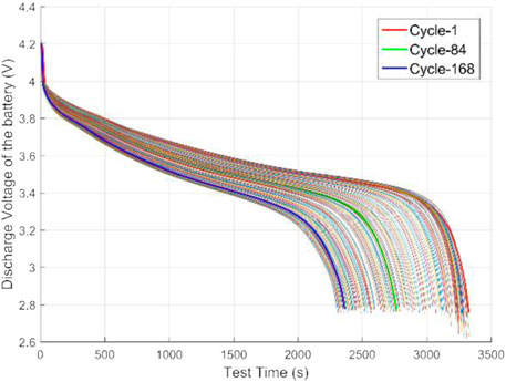
FIGURE 1. Discharge voltage curve of battery #1.

FIGURE 2

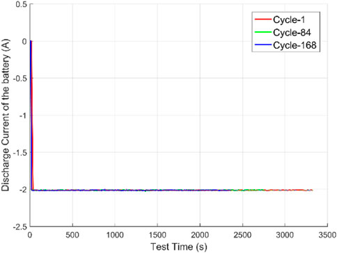
FIGURE 2. Discharge current curve of battery #1.

FIGURE 3

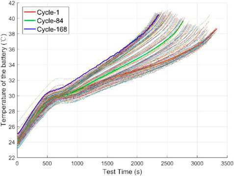
FIGURE 3. Discharge temperature curve of battery #1.

FIGURE 4

FIGURE 4. Discharge SOC curve of battery #1.

FIGURE 5

FIGURE 5. Voltage at SOC = 100% of battery #1.

FIGURE 6

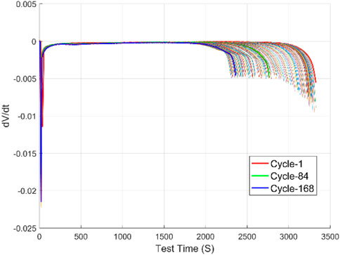
FIGURE 6. Discharge voltage rate of battery #1.

Figure 1 shows the discharge voltage curve of battery #1, and Figure 6 shows the discharge voltage drop rate curve of battery #1. It can be seen that in a single discharge process, the battery voltage drops rapidly at first, then enters a stable decline period, and finally drops rapidly again when the discharge process is near the end. In the discharge cycle process, the discharge voltage and the discharge voltage drop rate vary significantly in each cycle, indicating that both voltage and voltage change rate can be used as features to measure battery aging.

Figure 2 shows the discharge current curve of battery #1, which indicates that the battery is discharged at a constant current of 2A. It can be seen from the figure that as the number of cycles increases, the battery’s continuous discharge time decreases sharply. In the first discharge experiment, the discharge time lasted about 3,400 s, as shown by the red Cycle-1; in the 84th cycle experiment, the discharge time lasted about 2,800 s, as shown by the green Cycle-84; in the 168th cycle experiment, the discharge time lasted about 2,400 s, as shown by the blue Cycle-168. As the battery ages, the battery discharge time changes dramatically, so the battery discharge time can be used as a feature to measure battery aging. Since the experiment uses constant current discharge, this paper does not select current as a feature to measure battery aging.

Figure 3 shows the discharge temperature change curve of battery #1. It can be seen from the figure that as the number of cycles increases, the temperature in each discharge process increases continuously, which is caused by the increase of the internal impedance of the battery due to aging. For a single discharge process, the curve of discharge temperature change is not smooth and has many fluctuations. The temperature and impedance of the battery can both reflect the degree of battery aging significantly, but due to the difficulty of measuring battery impedance on electric vehicles, this paper does not choose impedance as a feature for battery SOH prediction. Figure 4 shows the discharge SOC change curve of battery #1. As the number of cycles increases, the rate of SOC decrease in each discharge process changes continuously, so the battery’s SOC can be used as a feature to measure battery aging.

Figure 5 shows the battery voltage corresponding to SOC = 100% at the beginning of each discharge cycle of battery #1. It can be seen from the figure that the change of the initial voltage is not regular, which is because the initial voltage is affected by factors such as battery internal resistance, ambient temperature, battery aging degree, etc. This paper also considers it as one of the input features to measure battery aging.

The SOH value of the battery reflects the current reliability of the battery. Accurate SOH prediction can enable the battery management system to manage each battery cell in the battery pack more effectively, especially the battery aging, effectively maintain the safety of the electric vehicle during operation, alleviate the driver’s driving anxiety, and help to accurately predict the remaining driving range of the electric vehicle. The SOH definition in this paper is: $\text{SOH}=Q_{\max }/Q_{rated}\times 100\%$, where $Q_{\max }$ is the maximum available capacity of the battery at the current state, and $Q_{\text{rated}}$ is the rated capacity of the battery. Figure 7 shows the battery SOH value corresponding to each cycle of battery #1 and battery #2, which reflects the degree of battery aging. It can be seen that as the number of cycles increases, SOH shows a downward trend overall, but has large fluctuations in the decline process, showing strong nonlinear characteristics.

FIGURE 7

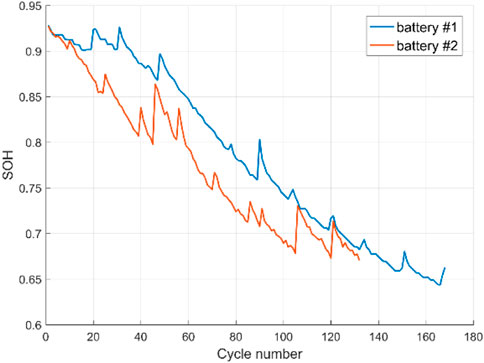
FIGURE 7. SOH of battery #1 and battery #2.

3.2 Decision tree analysis

The features such as voltage, discharge time, temperature, SOC, voltage at SOC = 100%, and voltage rate collected during the battery discharge process in Section 3.1 were analyzed using the decision tree to obtain the eigenvalues and feature importance for each feature parameter. The cumulative feature importance of features is also calculated.

Figure 8 shows that the battery voltage at SOC = 100% has a much larger eigenvalue than other battery features. The eigenvalues of the battery voltage, temperature, discharge time, SOC, and discharge voltage rate are different, but not by much. These parameters are used by researchers for SOH estimation. This paper selects features with cumulative feature importance greater than 85%.

FIGURE 8

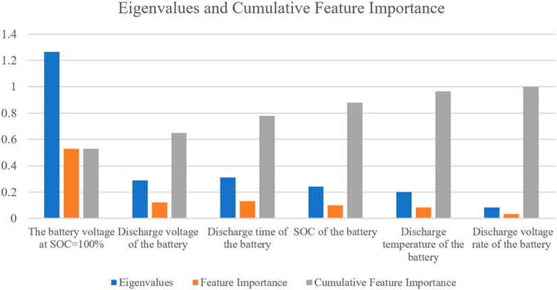
FIGURE 8. Eigenvalues and cumulative feature importance.

Based on the cumulative feature importance, five groups of SOH simulation experiments with different training set inputs are designed, which are: the first group with battery voltage at SOC = 100%, voltage, temperature, discharge time, SOC, discharge voltage rate; the second group with battery voltage at SOC = 100%, voltage, discharge time, SOC, discharge voltage rate; the third group with battery voltage at SOC = 100%, voltage, temperature, discharge time, SOC; the fourth group with battery voltage at SOC = 100%, voltage, temperature, discharge time; the fifth group with battery voltage at SOC = 100%, voltage, discharge time, SOC; and conduct simulation experiments to test the influence of battery feature parameter selection on battery SOH prediction.

3.3 The original SVR and improved SVR simulation process

The simulation procedure of the original SVR algorithm consists of the following steps. The first step is to reduce the dimensionality of the data obtained from the NASA battery experiment. The size of the sample data collected during the discharge process of battery #1 is $X\times 45205$, where $X$ represents the number of battery features to be selected, and the number of points collected in each discharge cycle is more than 100. If the size of the training set $X\times 31643$ is selected according to the traditional SVR training method, then the time required for an SVR training process is about 30 days based on my computer configuration. Therefore, the size of the training set needs to be simplified. This paper selects 100 points for each discharge cycle, and the corresponding SOC for each point is 1-100%. If there is no accurate SOC corresponding point, select the closest SOC. After the initial simplification, the size of the sample data becomes $X\times 16800$, and the size of the training set is $X\times 11760$. The second step is to normalize the three sets of experimental data collected to eliminate the dimension problem. The third step is to perform SVR training, which takes about 16 hours to obtain the corresponding regression prediction model.

The improved SVR algorithm simulation process is shown in Section 2.3, where the parameters are selected as described below. When $\tau =0.04$, the gap between the smooth loss function and the original function is less than 0.028 (Zheng, 2015), so in this paper we select $\mathrm{m}=25$, $\mathrm{M}=30$, $C=2000$, $\epsilon =0.5$, $\eta =0.001$. Both the improved and the original SVR use the Gaussian kernel as the kernel function, $K\left(\mathit{u},\mathit{v}\right)=\exp \left(-{‖\mathit{u}-\mathit{v}‖}^2/2{\sigma }^2\right)$, where $\sigma =5$. The improved and original SVR select the same size of training set and test set, and use mean square error (MSE) to evaluate the prediction accuracy on the test set, $\mathrm{M}\mathrm{S}\mathrm{E}=\frac{1}{N}{\sum }_{i=1}^N\left(f\left({\mathit{x}}_i\right)-y_i\right)$.

The battery SOH estimation flow chart based on improved SVR is shown in Figure 9. The specific steps are as follows: 1) Obtain the original training samples of the simulation experiment from the NASA public data and reduce their dimensionality; 2) Perform decision tree analysis of battery SOH features to obtain cumulative feature importance; 3) According to the cumulative feature importance, conduct five groups of different training set input original SVR simulation experiments to obtain the most suitable feature input group; 4) Select the most suitable features as the input of the training set, and apply the improved SVR algorithm to conduct a simulation experiment to establish an improved SVR prediction model; 5) Input test data and use the improved SVR prediction model to obtain the predicted SOH results.

FIGURE 9

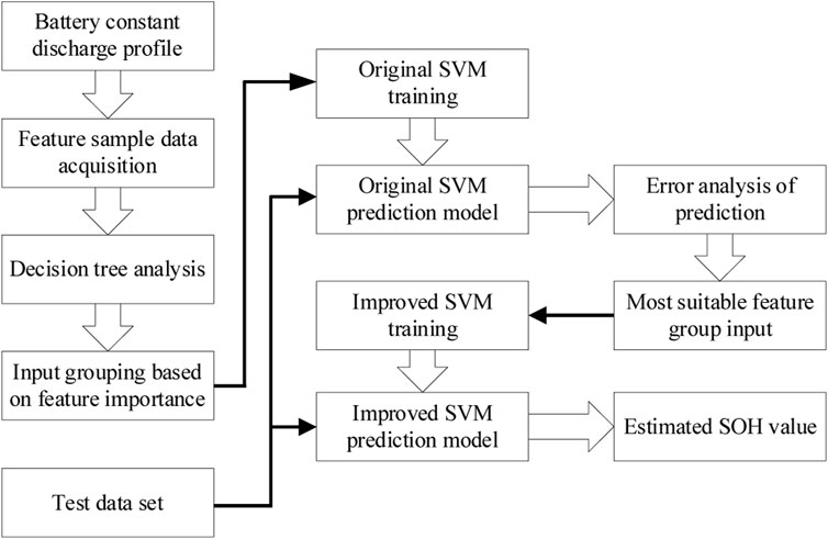
FIGURE 9. Battery SOH flow chart based on improved SVR.

4 Results and analysis

4.1 Estimation results based on original SVR

According to the cumulative feature importance obtained by decision tree analysis, five groups of battery SOH simulation experiments with original SVR algorithm are conducted. The input of the five experiments follows Section 3.2 and the output is the battery SOH value. The parameters of the original SVR model are obtained by grid search and cross-validation methods. The training set used to predict the SOH of the battery #2 is randomly selected from the reduced sample set of battery #1 set and the size of the training set is set as $X\times 11760$ in Section 3.33. The SOH curves of battery #1 and battery #2 batteries are shown in Figure 7. It can be seen from Figure 7 that both batteries have a decreasing SOH value with the increase of cycle test times, but #2 battery ages faster than #1 battery. When SOH is less than 0.7, it means that the battery has reached the scrap standard and needs to be replaced with a new one (Qin et al., 2015). Nine SOC intervals are selected to evaluate the original SVR model performance. Figure 10 compares the simulation results of the five experiments with the actual values of battery SOH prediction. To better graphically demonstrate the model estimation errors for the nine SOC intervals, the root mean square error (RMSE) is used, $\mathrm{R}\mathrm{M}\mathrm{S}\mathrm{E}=\sqrt{\frac{1}{N}{\sum }_{i=1}^N\left(f\left({\mathit{x}}_i\right)-y_i\right)}$.

FIGURE 10

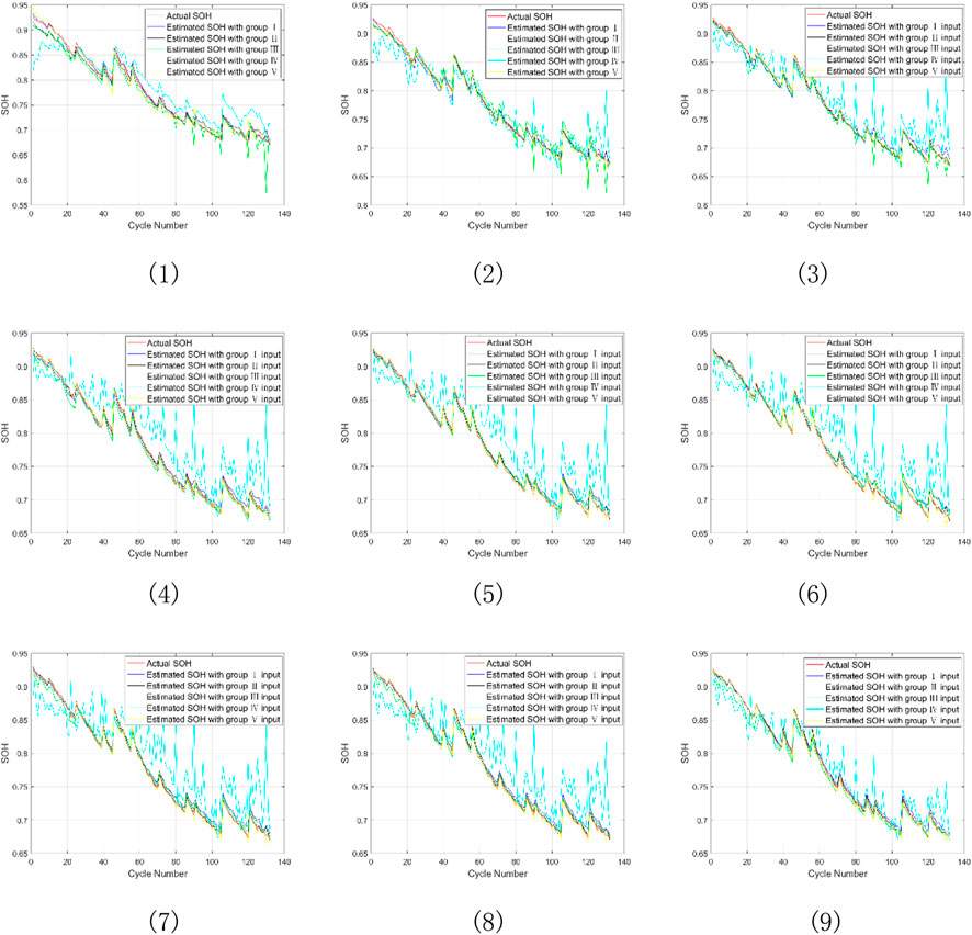
FIGURE 10. Estimation of SOH for battery #2 under nine SOC intervals (1) SOC change (100%–10%), (2) SOC change (100%–20%), (3) SOC change (100%–30%), (4) SOC change (100%–40%), (5) SOC change (100%–50%), (6) SOC change (100%–60%), (7) SOC change (100%–70%), (8) SOC change (100%–80%), (9) SOC change (100%–90%).

Figure 10, 11 show the simulation results and RMSE of battery SOH estimation in nine SOC interval segments under five groups of inputs. The fourth group of inputs without battery SOC feature has the largest fluctuation and RMSE, and is inaccurate for SOH prediction. Therefore, the fourth group of inputs is not suitable for predicting battery SOH. The first and third groups of inputs have similar prediction results and RMSE, with the first group slightly better than the third group, but both are worse than the second and fifth groups. The second group of inputs obtains the best prediction results and RMSE, followed by the fifth group. These results show that excluding battery temperature from the input features improves the prediction accuracy because the collected battery temperature has frequent fluctuations in each discharge cycle. Therefore, the temperature collected in this experiment is not suitable for predicting battery SOH. The Figures also show that the SOH estimation error is large when the initial $\Delta$ SOC is low, due to the steep discharge voltage drop rate in the SOC (100%–90%) interval. The error decreases in the SOC (100%–90%) - SOC (100%–50%) interval, because the discharge voltage drop rate is flat, and the discharge voltage decreases steadily. The error fluctuates slightly in the SOC (100%–50%) - SOC (100%–10%) interval, because the discharge voltage drop rate changes from flat to steep grade, and the discharge voltage also changes from steady decline to fast decline. In general, the SOH estimation error decreases as SOC increases.

FIGURE 11

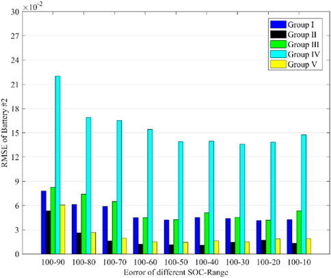
FIGURE 11. RMSE for battery #2 under nine SOC intervals.

Table 1 shows the average MSE and RMSE of the battery SOH simulation for the five groups of inputs in nine SOC intervals. The AVG_MSE and AVG_RMSE in the table represent the average MSE and RMSE of the nine SOC intervals, respectively. As shown in Table 1, the fourth group of inputs has the highest AVG_MSE and AVG_RMSE, whereas the second group of inputs has the lowest. The fifth group of inputs is similar to the second group input in terms of AVG_MSE and AVG_RMSE. Both the second and fifth groups of inputs are suitable for SOH prediction, but the fifth group of inputs requires fewer features to be collected. Therefore, we suggest using the fifth group of inputs as the training set feature input for SVR-based battery SOH prediction.

TABLE 1

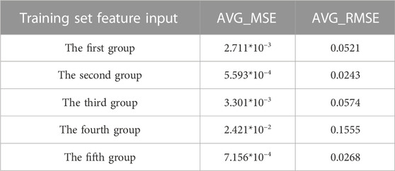
TABLE 1. Average prediction error of original SVR.

4.2 Estimation results based on improved SVR

The fifth group of inputs is used to predict SOH with the improved SVR algorithm. Both the improved and the original SVR have a training set size of 0.7 times the sample set size, which is 11,760 × 4. In this paper, an ASUS computer is used in the simulation, the CPU is an I7-6500U, the memory is 12 GB, the solid-state hard disk is 250 GB, and the system is WIN10.

Figure 12, 13 compare the simulation results and RMSE of battery SOH estimation using the improved SVR and the original SVR in nine SOC intervals. As shown in Figure 12, 13, the improved SVR has slightly lower prediction accuracy than the original SVR. The RMSE difference is 0.0342 in SOC (100%–90%) and less than 0.01 in the other SOC intervals. The improved SVR is a slight trade-off comparable to the original SVR in terms of prediction performance.

FIGURE 12

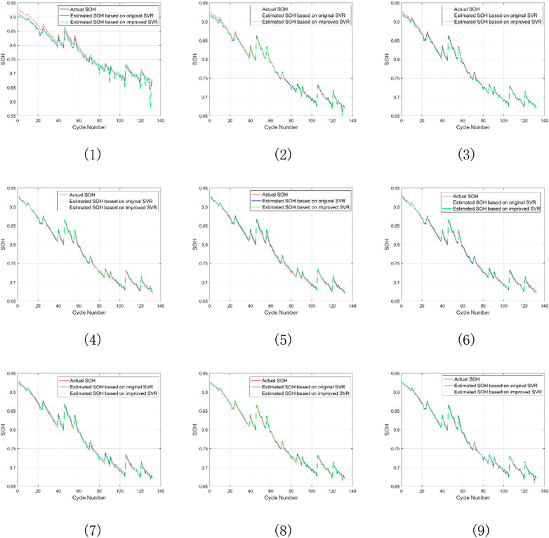
FIGURE 12. SOH estimation of battery #2 based on improved SVR and original SVR algorithms under nine SOC intervals (1) SOC change (100%–10%), (2) SOC change (100%–20%), (3) SOC change (100%–30%), (4) SOC change (100%–40%), (5) SOC change (100%–50%), (6) SOC change (100%–60%), (7) SOC change (100%–70%), (8) SOC change (100%–80%), (9) SOC change (100%–90%).

FIGURE 13

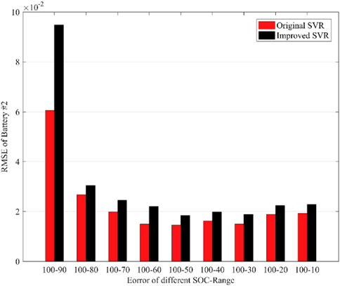
FIGURE 13. RMSE of battery #2 based on improved SVR and original SVR algorithms under nine SOC intervals.

Table 2 summarizes the AVG_MSE, AVG_RMSE and the training time of the improved SVR and the original SVR with the fifth group of inputs. The improved SVR has slightly lower accuracy than the original SVR, with a 0.00078438 higher AVG_MSE and a 0.0101 higher AVG_RMSE. This is because the improved SVR uses a smooth function to approximate the original SVR loss function, transforming the original quadratic programming into a convex unconstrained minimization problem. However, the improved SVR algorithm training time is much shorter, with an 83.9% lower training time than the original SVR algorithm. This is because the improved SVR algorithm uses the conjugate gradient method to solve the convex unconstrained minimization problem, which is faster than grid search as it does not need to traverse all points in the grid.

TABLE 2

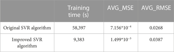
TABLE 2. Comparison of training time and prediction accuracy of original SVR and improved SVR.

4.3 Comparison with other algorithms

Using battery #1 as the training dataset, we predict the SOH of battery #2 with a SOC interval of 100%–10% for the test set. Table 3 compares the SOH prediction errors of the improved SVR, the original SVR, and other machine learning algorithms from the literature (Khumprom and Yodo, 2019; Li et al., 2021), namely, k-Nearest Neighbors (k-NN), Linear Regression (LR), Artificial Neural Networks (ANN) and PSO-SVM. As Table 3 shows, the improved SVR has lower MSE and RMSE than k-NN, LR, and ANN, it indicates that the improved SVR has good predictive performance for battery SOH. Since the improved SVR focuses more on reducing the training time of SVR, there is an obvious drop in simulation accuracy compared to the PSO-SVR which is dedicated to improving the accuracy of SVR simulation. Compared with the original SVR, the improved SVR has slightly lower accuracy but significantly shorter simulation time.

TABLE 3

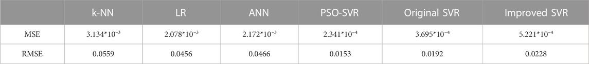
TABLE 3. Comparison of different SOH prediction algorithms.

5 Conclusion

The accurate prediction of battery SOH is one of the key functions of electric vehicle BMS. In this paper, feature data sets are extracted from NASA’s battery aging experiments and dimensionality reduction is performed on them. The decision tree algorithm is used to group the features and perform the original SVR algorithm simulation on each group. The simulation results show that four feature inputs can meet the desired SOH prediction accuracy requirements: voltage at SOC = 100%, voltage, discharge time, and SOC. The original SVR model is fitted by solving the dual of the original constrained optimization problem, resulting in a quadratic programming problem that is computationally very time-consuming to solve. To reduce the long training time of original SVR for large sample data sets, an improved SVR algorithm is proposed. The improved SVR model is fitted by directly minimizing the primal form of the optimization problem. Since the original SVR objective function is not differentiable, we introduce a smoothing function to approximate the objective function of the original SVR, transforming the original quadratic programming problem into a convex unconstrained minimization problem, and subsequently solving the smoothed approximate objective function in a sequential minimum optimization manner using conjugate gradient algorithm. The improved SVR algorithm is applied to the four feature inputs. The simulation results show that the improved SVR algorithm saves 83.9% of the training time compared to the original SVR algorithm, with a slight trade-off in prediction accuracy. In future work, we plan to use data sets collected from real vehicles and real vehicle verification tests.

Data availability statement

The datasets presented in this study can be found in online repositories. The names of the repository/repositories and accession number(s) can be found below: https://ti.arc.nasa.gov/tech/dash/groups/pcoe/prognostic-data-repository/.

Author contributions

LJQ guided the direction of the research and provided the research site; LX performed the simulations, analysis of the results, and writing of the paper; JC performed the verification and touch-up of the paper. All authors contributed to the article and approved the submitted version.

Funding

This work was supported in part by the National Natural Science Foundation, China, Under Grant No. 51875149.

Conflict of interest

The authors declare that the research was conducted in the absence of any commercial or financial relationships that could be construed as a potential conflict of interest.

Publisher’s note

All claims expressed in this article are solely those of the authors and do not necessarily represent those of their affiliated organizations, or those of the publisher, the editors and the reviewers. Any product that may be evaluated in this article, or claim that may be made by its manufacturer, is not guaranteed or endorsed by the publisher.

Supplementary material

The Supplementary Material for this article can be found online at: https://www.frontiersin.org/articles/10.3389/fenrg.2023.1218580/full#supplementary-material

References

Ali, M. U., Zafar, A., Nengroo, S. H., Hussain, S., Park, G. S., and Kim, H. J. (2019). Online remaining useful life prediction for lithium-ion batteries using partial discharge data features. Energies 12 (22), 4366. doi:10.3390/en12224366

CrossRef Full Text | Google Scholar

Andre, D., Appel, C., Soczka-Guth, T., and Sauer, D. U. (2013). Advanced mathematical methods of SOC and SOH estimation for lithium-ion batteries. J. power sources 224, 20–27. doi:10.1016/j.jpowsour.2012.10.001

CrossRef Full Text | Google Scholar

Berecibar, M., Gandiaga, I., Villarreal, I., Omar, N., Van Mierlo, J., and Van den Bossche, P. (2016). Critical review of state of health estimation methods of Li-ion batteries for real applications. Renew. Sustain. Energy Rev. 56, 572–587. doi:10.1016/j.rser.2015.11.042

CrossRef Full Text | Google Scholar

Chen, R. J., Hsu, C. W., Lu, T. F., and Teng, J. H. “Rapid SOH estimation for retired lead-acid batteries[C],” in IEEE International Future Energy Electronics Conference (IFEEC), Taipei, Taiwan, China, November 16-19, 2021, 1–4.

Google Scholar

Chen, Z., Sun, M., Shu, X., Xiao, R., and Shen, J. (2018). Online state of health estimation for lithium-ion batteries based on support vector machine. Appl. Sci. 8 (6), 925. doi:10.3390/app8060925

CrossRef Full Text | Google Scholar

Chiang, Y. H., Sean, W. Y., and Ke, J. C. (2011). Online estimation of internal resistance and open-circuit voltage of lithium-ion batteries in electric vehicles. J. Power Sources 196 (8), 3921–3932. doi:10.1016/j.jpowsour.2011.01.005

CrossRef Full Text | Google Scholar

Corey, G. P. “Batteries for stationary standby and for stationary cycling applications part 6: Alternative electricity storage technologies[C],” in Proceedings of the Power Engineering Society General Meeting, Toronto, ON, Canada, July 13–17, 2003, 164–169.

Google Scholar

Cortes, C., and Vapnik, V. (1995). Support-vector networks. Mach. Learn. 20, 273–297. doi:10.1007/bf00994018

CrossRef Full Text | Google Scholar

Deng, Z., Hu, X., Li, P., Lin, X., and Bian, X. (2021). Data-driven battery state of health estimation based on random partial charging data. IEEE Trans. Power Electron. 37 (5), 5021–5031. doi:10.1109/tpel.2021.3134701

CrossRef Full Text | Google Scholar

Deng, Z., Lin, X., Cai, J., and Hu, X. (2022). Battery health estimation with degradation pattern recognition and transfer learning. J. Power Sources 525, 231027. doi:10.1016/j.jpowsour.2022.231027

CrossRef Full Text | Google Scholar

Feng, X., Weng, C., He, X., Han, X., Lu, L., Ren, D., et al. (2019). Online state-of-health estimation for Li-ion battery using partial charging segment based on support vector machine. IEEE Trans. Veh. Technol. 68 (9), 8583–8592. doi:10.1109/tvt.2019.2927120

CrossRef Full Text | Google Scholar

Kheirkhah-Rad, E., and Moeini-Aghtaie, M. “A novel data-driven SOH prediction model for lithium-ion batteries[C],” in IEEE 31st Australasian Universities Power Engineering Conference (AUPEC), Perth, Australia, September 26-30, 2021, 1–6.

Google Scholar

Khumprom, P., and Yodo, N. (2019). A data-driven predictive prognostic model for lithium-ion batteries based on a deep learning algorithm. Energies 12 (4), 660. doi:10.3390/en12040660

CrossRef Full Text | Google Scholar

Lawder, M. T., Suthar, B., Northrop, P. W. C., De, S., Hoff, C. M., Leitermann, O., et al. (2014). Battery energy storage system (BESS) and battery management system (BMS) for grid-scale applications. Proc. IEEE 102 (6), 1014–1030. doi:10.1109/jproc.2014.2317451

CrossRef Full Text | Google Scholar

Lee, Y. J., and Mangasarian, O. L. (2001). Ssvm: A smooth support vector machine for classification[J]. Comput. Optim. Appl. 20, 5–22. doi:10.1023/a:1011215321374

CrossRef Full Text | Google Scholar

Li, R., Li, W., Zhang, H., Zhou, Y., and Tian, W. (2021). On-line estimation method of lithium-ion battery health status based on PSO-SVM[J]. Front. Energy Res. 9, 693249. doi:10.3389/fenrg.2021.693249

CrossRef Full Text | Google Scholar

Li, S. E., Wang, B., Peng, H., and Hu, X. (2014). An electrochemistry-based impedance model for lithium-ion batteries. J. Power Sources 258, 9–18. doi:10.1016/j.jpowsour.2014.02.045

CrossRef Full Text | Google Scholar

Liu, X., Li, J., Yao, Z., Wang, Z., Si, R., and Diao, Y. (2022). Research on battery SOH estimation algorithm of energy storage frequency modulation system. Energy Rep. 8, 217–223. doi:10.1016/j.egyr.2021.11.015

CrossRef Full Text | Google Scholar

Patil, M. A., Tagade, P., Hariharan, K. S., Kolake, S. M., Song, T., Yeo, T., et al. (2015). A novel multistage Support Vector Machine based approach for Li ion battery remaining useful life estimation. Appl. Energy 159, 285–297. doi:10.1016/j.apenergy.2015.08.119

CrossRef Full Text | Google Scholar

Pirmana, V., Alisjahbana, A. S., Yusuf, A. A., Hoekstra, R., and Tukker, A. (2023). Economic and environmental impact of electric vehicles production in Indonesia[J]. Clean Technol. Environ. Policy, 1–15. doi:10.1007/s10098-023-02475-6

CrossRef Full Text | Google Scholar

Qian, K. F., and Liu, X. T. (2021). Hybrid optimization strategy for lithium-ion battery's State of Charge/Health using joint of dual Kalman filter and Modified Sine-cosine Algorithm. J. Energy Storage 44, 103319. doi:10.1016/j.est.2021.103319

CrossRef Full Text | Google Scholar

Qin, T., Zeng, S., and Guo, J. (2015). Robust prognostics for state of health estimation of lithium-ion batteries based on an improved PSO–SVR model. Microelectron. Reliab. 55 (9-10), 1280–1284. doi:10.1016/j.microrel.2015.06.133

CrossRef Full Text | Google Scholar

Severson, K. A., Attia, P. M., Jin, N., Perkins, N., Jiang, B., Yang, Z., et al. (2019). Data-driven prediction of battery cycle life before capacity degradation. Nat. Energy 4 (5), 383–391. doi:10.1038/s41560-019-0356-8

CrossRef Full Text | Google Scholar

Shen, S., Sadoughi, M., Chen, X., Hong, M., and Hu, C. (2019). A deep learning method for online capacity estimation of lithium-ion batteries. J. Energy Storage 25, 100817. doi:10.1016/j.est.2019.100817

CrossRef Full Text | Google Scholar

Smola, A. J., and Schölkopf, B. (2004). A tutorial on support vector regression. Statistics Comput. 14, 199–222. doi:10.1023/b:stco.0000035301.49549.88

CrossRef Full Text | Google Scholar

Vichard, L., Ravey, A., Venet, P., Harel, F., Pelissier, S., and Hissel, D. (2021). A method to estimate battery SOH indicators based on vehicle operating data only. Energy 225, 120235. doi:10.1016/j.energy.2021.120235

CrossRef Full Text | Google Scholar

Vidal, C., Malysz, P., Kollmeyer, P., and Emadi, A. (2020). Machine learning applied to electrified vehicle battery state of charge and state of health estimation: State-of-the-Art. IEEE Access 8, 52796–52814. doi:10.1109/access.2020.2980961

CrossRef Full Text | Google Scholar

Wang, S., Fan, Y., Jin, S., Takyi-Aninakwa, P., and Fernandez, C. (2023). Improved anti-noise adaptive long short-term memory neural network modeling for the robust remaining useful life prediction of lithium-ion batteries. Reliab. Eng. Syst. Saf. 230, 108920. doi:10.1016/j.ress.2022.108920

CrossRef Full Text | Google Scholar

Wang, S., Ren, P., Takyi-Aninakwa, P., Jin, S., and Fernandez, C. (2022a). A critical review of improved deep convolutional neural network for multi-timescale state prediction of lithium-ion batteries. Energies 15 (14), 5053. doi:10.3390/en15145053

CrossRef Full Text | Google Scholar

Wang, S., Takyi-Aninakwa, P., Jin, S., Yu, C., Fernandez, C., and Stroe, D. I. (2022b). An improved feedforward-long short-term memory modeling method for the whole-life-cycle state of charge prediction of lithium-ion batteries considering current-voltage-temperature variation. Energy 254, 124224. doi:10.1016/j.energy.2022.124224

CrossRef Full Text | Google Scholar

Wang, Z., Ma, J., and Zhang, L. (2017). State-of-Health estimation for lithium-ion batteries based on the multi-island genetic algorithm and the Gaussian process regression. IEEE Access 5, 21286–21295. doi:10.1109/access.2017.2759094

CrossRef Full Text | Google Scholar

Wang, Z., Zeng, S., Guo, J., and Qin, T. (2019). State of health estimation of lithium-ion batteries based on the constant voltage charging curve. Energy 167, 661–669. doi:10.1016/j.energy.2018.11.008

CrossRef Full Text | Google Scholar

Weng, C., Sun, J., and Peng, H. (2014). A unified open-circuit-voltage model of lithium-ion batteries for state-of-charge estimation and state-of-health monitoring. J. power Sources 258, 228–237. doi:10.1016/j.jpowsour.2014.02.026

CrossRef Full Text | Google Scholar

Xiong, W., Mo, Y., and Yan, C. (2020). Online state-of-health estimation for second-use lithium-ion batteries based on weighted least squares support vector machine. IEEE Access 9, 1870–1881. doi:10.1109/access.2020.3026552

CrossRef Full Text | Google Scholar

Yang, D., Zhang, X., Pan, R., Wang, Y., and Chen, Z. (2018). A novel Gaussian process regression model for state-of-health estimation of lithium-ion battery using charging curve. J. Power Sources 384, 387–395. doi:10.1016/j.jpowsour.2018.03.015

CrossRef Full Text | Google Scholar

Yang, R., Zhang, X., Liu, G., and Hou, S. “State of health estimation for power battery based on support vector regression and particle swarm optimization method[C],” in IEEE 40th Chinese Control Conference (CCC), Shanghai, China, July 26-28, 2021, 6281–6288.

Google Scholar

Zhang, Y., Xiong, R., He, H., and Pecht, M. G. (2018). Long short-term memory recurrent neural network for remaining useful life prediction of lithium-ion batteries. IEEE Trans. Veh. Technol. 67 (7), 5695–5705. doi:10.1109/tvt.2018.2805189

CrossRef Full Text | Google Scholar

Zheng, S. (2015). A fast algorithm for training support vector regression via smoothed primal function minimization. Int. J. Mach. Learn. Cybern. 6, 155–166. doi:10.1007/s13042-013-0200-6

CrossRef Full Text | Google Scholar

Zheng, S. (2011). Gradient descent algorithms for quantile regression with smooth approximation. Int. J. Mach. Learn. Cybern. 2, 191–207. doi:10.1007/s13042-011-0031-2

CrossRef Full Text | Google Scholar

Zhuang, H. M., and Xiao, J. (2014). VRLA battery SOH estimation based on WCPSO-lvsvm. Appl. Mech. Mater. 628, 396–400. doi:10.4028/www.scientific.net/amm.628.396

CrossRef Full Text | Google Scholar