 Xianqiang Zeng1
 Yun Zhou
 Hengjie Li
94% of researchers rate our articles as excellent or good
Learn more about the work of our research integrity team to safeguard the quality of each article we publish.
Find out more
ORIGINAL RESEARCH article
Front. Energy Res. , 10 July 2023
Sec. Process and Energy Systems Engineering
Volume 11 - 2023 | https://doi.org/10.3389/fenrg.2023.1218035
This article is part of the Research Topic Key Technologies for Hybrid Energy System Planning and Operation View all 10 articles
Under the “carbon peaking and carbon neutrality” development strategy, in order to suppress load fluctuations and promote renewable energy consumptions in the regional integrated energy system involving concentrating solar power stations, a double-layer optimization model based on the improved non-dominated sorting genetic algorithm-II (NSGA-II) and mixed integer linear programming (MILP) is proposed. The upper layer completes the capacity configuration process based on multiple objectives to minimize the annual planning cost and the net emission of pollutants. The lower layer is designed to minimize the annual operating cost and optimize the output of the devices and the load curves through the participation of the integrated demand response process for flexible loads and the whole process of carbon emission including carbon capture, carbon utilization, and carbon trading mechanisms to obtain the best operating plan. The final results indicate that the participation of concentrating solar power stations can improve the level of coordinated optimization, and the improved NSGA-II is stronger than the conventional one in convergence ability. Besides, considering the whole process of carbon emission and integrated demand response is capable of decreasing the annual operating cost and net carbon emission to improve the economy and environmental protection of the system significantly.
In recent years, environmental problems have become more serious, so the exploration of clean energy will become an inevitable trend in the future development (Fan et al., 2021). The regional integrated energy system (RIES) breaks the barrier between energy planning and operation, and its internal multi-energy coupling equipment can realize energy gradient utilization (Chen et al., 2022; Wang B. et al., 2022), which plays a huge part in realizing the goal of promoting economic and environmental benefits.
In the field of RIES low-carbon operation, relevant studies mostly focus on the regulatory means and economic mechanisms such as carbon capture, carbon storage, and carbon trading. In the work of Dong et al. (2022), a carbon capture model combined with power-to-gas and gas-fired units was installed, which effectively minimized the carbon cost of the total system through the improved energy hub formulation. In the work of Zhang D. et al. (2021), a carbon storage device with pollutant treatments and carbon capture systems (CCSs) was regarded as the structure of an evolutionary IES, which significantly improved renewable energy penetration under different specifications. In the work of Yan et al. (2023), a seasonal-stepped carbon trading mechanism was introduced, and the impacts of economics on optimal dispatch are also considered comprehensively. However, few studies have been conducted on cost-effective carbon utilization processes compared with costly carbon storage processes.
Research on the participation of flexible loads in integrated demand response (IDR) is generally classified into price type, incentive type, and substitution type according to their guiding modes. Yang et al. (2020) divided the IDR into price-based and alternative parts with the process of rolling optimization and finally showed that the aforementioned method can restrain the fluctuation of the loads. Wang et al. (2021) put forward an uncertain model of the demand response through the energy coupling matrices to investigate the impact of price incentives under different scenarios in the RIES to realize the improvement in the load profile. Shao et al. (2019) promoted the IDR to smart buildings and then developed a real-time exchange market with the feasible region method to adjust energy consumption behaviors. Zhang et al. (2022) proposed a multi-objective model considering two-dimensional demand responses with spatiotemporal coupling characteristics to obtain the control strategy among different benefit weights. However, most research on IDR focuses on electricity and heat at present, while cool energy and gas energy are rarely considered.
In addition, with the steady development of concentrating solar power (CSP) in renewable energy, photothermal power generation has gradually attracted wide attention for its advantages of good controllability and high adjustability. Zhao et al. (2019) analyzed the influences of wind power uncertainty on optimal dispatch and put forward a stochastic model for the combination of the CSP stations and wind farms according to the simulation results. In the work of Zhang G. et al. (2021), CSP stations were introduced as cogenerated units and a multi-dispatch method for the RIES was proposed. The results show that the participation of CSP stations can reduce operating costs. On the premise of considering operating cost, Jiang et al. (2020) built an exchange model between CSP stations and energy markets to participate in DR programs, which significantly improved the energy operating efficiency through the price elasticity matrix of the electrical and the heat loads. However, the existing literature has generally ignored the potential of CSP stations operating in conjunction with the aforementioned CCS.
In view of the problems mentioned previously, the main contributions of this paper are shown as follows:
1) An energy hub (EH) with the participation of the CSP station and the whole process of carbon emission including carbon capture, carbon utilization, and carbon trading is established by considering the power-to-gas equipment.
2) The analysis includes flexible loads such as electricity, heat, cooling, and gas and successively elaborates them for the uncontrollable loads, transferable loads, curtailable loads, and fungible loads, which are refined to reflect the IDR.
3) A double-layer optimization model of improved NSGA-II and MILP is constructed. The upper layer takes the annual planning cost and net pollutant discharge as the target for device selection and capacity configuration through the improved NSGA-II, while the lower layer regards the annual operating cost as the target to optimize the output of each device through the Cplex solver.
This paper is organized as follows. In Section 2, the basic structure and the operating principle of the RIES are introduced. Section 3 is focused on the expression of the proposed CSP station, the whole process of carbon emission, and the IDR. In Section 4, a double-layer model considering the solving methods is developed to realize the optimized process. Case studies are conducted in Section 5, in which the proposed model is simulated under different scenarios. At last, the conclusions are given in Section 6.
This paper focuses on the RIES shown in Figure 1. The system includes the wind turbine (WT), photovoltaic (PV), CSP station, electric boiler (EB), electric chiller (EC), waste heat boiler (WHB), absorption chiller (AC), gas turbine (GT), gas boiler (GB), carbon capture system (CCS), power to gas (P2G), and storage battery (SB). The energy input sources of the RIES are electricity and natural gas, and the loads include electricity, heat, cooling, and gas. The CSP station can be regarded as cogenerated equipment. Similarly, GT consumes natural gas to generate heat, which can be recovered by WHB. For the CCS, the CO2 captured is mainly from coal-fired plants in the power grid and gas-fired units (GT and GB) in the RIES. The power consumption of P2G can be supplied by abandoned wind and light, thus realizing the absorptive process of renewable energy. The entered electricity and natural gas of the EH can be purchased from power grid companies and natural gas companies, respectively, and then reasonably distributed to various energy conversion equipment and user-side loads.
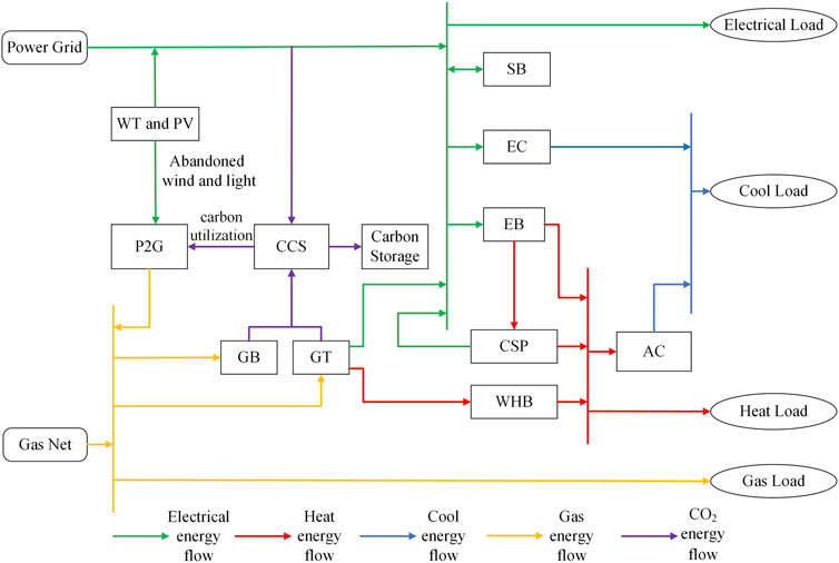
FIGURE 1. Structure diagram of the RIES.
The conventional devices of the RIES mainly include gas-fired units, EB, EC, AC, and WHB. The models are shown as follows:
where
As an emerging form of power generation in recent years, the CSP station is mainly divided into tower type, trough type, disk type, and linear Fresnel type, among which the tower type has been widely used in engineering practice for its advantages of strong economy and good performance (Gorman et al., 2021). In this paper, the heat storage tank and EB are aggregated to model the internal and external energy transfer relationships of the tower-type CSP station. The typical structure is shown in Figure 2.
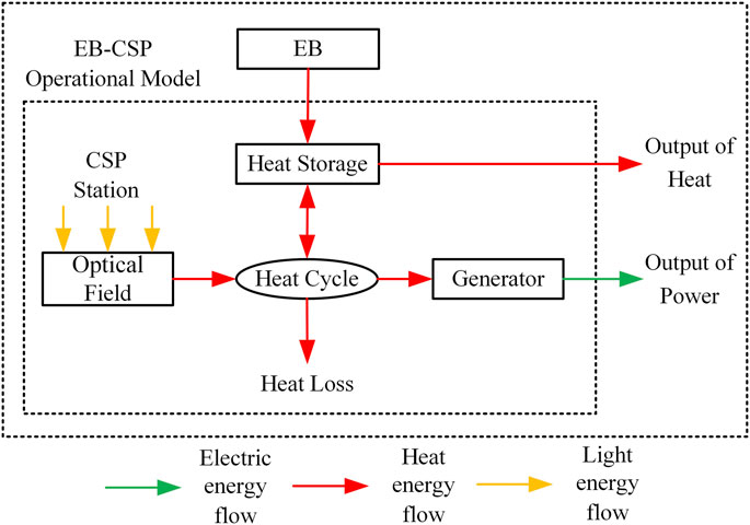
FIGURE 2. EB–CSP framework.
The heat energy collected by the heat collector in the optical field can be stored in the heat storage tank through the heat transfer mediums, and it can also be used to generate electricity through the heat cycle. The expression of photothermal conversion of the heat collector is shown as follows:
where
The heat storage tank can store the converted heat energy and can also release the heat energy to meet the generation demand or directly supply the heat to the load side. The model of the heat storage tank is shown in the following formula:
where
To keep the CSP station in stable operation after the participation of EB, its internal heat cycle must meet the following relations:
where
The generation power of the CSP station mainly comes from the heating power of the heat collector and the heat storage tank:
where
The heat energy provided to the load side is expressed as follows:
where
In this paper, P2G can absorb the power of abandoned wind and light, which is used to generate natural gas. The energy consumption of P2G is shown in the following equation:
where
The amount of CO2 consumed in P2G can be formulated as follows:
where
The natural gas produced by P2G can be calculated as follows:
The CCS mainly includes the absorption tower, regeneration tower, compressor, and other structural units. The absorber uses a specific solution to absorb CO2 from the flue gas and transfers it to the regenerator, where it is heated and separated. Then, CO2 is compressed in the compressor for transporting. Therefore, the energy consumption of carbon capture and gas treatment generated by the three links mentioned previously are the main sources of the total energy consumption in the CCS (Yan et al., 2017), whose expression is shown as follows:
where
where
The capacity of the flue gas storage tank is shown as follows:
where
In this paper, a combined operation strategy of wind power–photovoltaic–CSP–carbon capture based on the participation of the CCS and new energy units is proposed. The output of new energy units is partly used for carbon capture, partly used for flue gas treatment, and the rest is transported to the power grid. The energy consumption process of the carbon capture is presented in Figure 3 in the following section, and the energy consumption process of the flue gas treatment is similarly omitted.
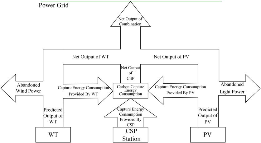
FIGURE 3. Flow chart of carbon capture energy.
The expression of joint operation is shown as follows:
where
Carbon utilization refers to sending captured CO2 into P2G to participate in the synthesis of CH4 as its raw material. This process can decrease the carbon storage cost and increase the operating flexibility of P2G. The carbon utilization process satisfies the following relations:
where
The carbon trading mechanism regards the carbon emission as a commodity and controls it through the trading of carbon emission rights between producers and markets. If the actual carbon emission is lower than the allocated, the surplus quotas can be sold to carbon trading markets. Otherwise, the corresponding quotas need to be purchased additionally (Wang X. et al., 2022).
1) Quota models of carbon emission
Carbon emission quota is the amount of emission allowance allocated by the regulatory authorities to each carbon source within the RIES, which varies according to the type of equipment (Chen et al., 2021). In this paper, there are two main carbon sources, namely, coal-fired power plants in the power grid (superior purchasing power) and gas-fired units of the system (GT and GB). Then, the quota models of carbon emission can be expressed as follows:
where
2) Practical models of carbon emission
Since the CCS can absorb CO2, the actual model of carbon emission after considering it can be expressed as follows:
where
3) Ladder-type carbon trading
After getting the quotas of carbon emission and the practical model through the process previously, the transaction volume of carbon emission rights that participate in trading markets can be formulated as follows:
Compared with the traditional carbon trading mechanism, the ladder-type carbon trading mechanism has more strict controls over carbon emissions. The principle is dividing carbon emissions into multiple intervals through the stepped pricing method. With the increase in carbon emissions, the transaction cost within the corresponding interval will increase (Zhang et al., 2016; Fu et al., 2022; Li et al., 2022). Accordingly, the cost of ladder-type carbon trading can be expressed as follows:
where
IDR refers to the process in which users reasonably adjust energy-use modes and participate in energy interaction according to different energy prices or incentive mechanisms to optimize the load curves (Shao et al., 2021). Therefore, it is necessary to classify the loads first in the analysis of such problems. In addition to uncontrollable loads (invariable loads) in previous studies, the loads are divided into variable loads such as transferable loads, curtailable loads, and fungible loads in this paper. In addition, compared to conventional studies that only consider electrical and heat loads, this paper incorporates all types of loads involving electricity, heat, cooling, and gas into the IDR. Then, according to the characteristics of the variable loads mentioned previously, the process of IDR involved in this paper is able to divide it into the price type and the substitutable type.
Since different types of loads have variant sensitivities to the same price signal, this paper divides the loads involved in the price-based demand response into curtailable loads (CLs) and transferable loads (TLs) and then builds the models of them in turn.
1) Properties and modeling for CL
CL uses the price-demand elasticity matrix to describe its characteristics. In allusion to the t line and the j column element
where
Then, the CL variation of class
where
2) Properties and modeling for TL
TL can realize flexible controls of working hours and power at different periods under the total load unchanged premise according to the energy prices of users’ own demand response. Taking time-sharing energy prices and incentive measures as signals, users can be guided to transfer the peak loads to the normal or trough period (Azzam et al., 2023). Similarly, after expressing the characteristics of IDR in the price-demand elasticity matrix, the TL variation in class
where
For a certain type of the heat load that can be directly supplied by heat or electricity (electricity to heat), the electrical energy can be consumed in periods of low electricity prices, while the heat energy can be directly consumed in periods of high electricity prices to meet different needs so as to realize the mutual substitution between the electrical and heat energy. The fungible load (FL) model can be expressed as follows:
where
Through the IDR process mentioned previously, the following conditions of load balance can be obtained as follows:
where
where
Based on the RIES with the participation of CSP stations as shown in Figure 1, this paper establishes a double-layer optimization model that considers the whole process of carbon emission and the IDR to demonstrate the innovations. The upper layer randomly generates the planned capacities of the devices and transmits them to the lower layer. The lower layer constrains the output of the devices and transmits the results back to the upper layer. Finally, the upper layer revises the capacity configuration of each device again. The iterative process between the upper layer and the lower layer leads to the most optimal configuration and the lowest annual operating cost of the RIES.
The upper model aims at minimizing the annual planning cost and the annual net pollutant emission of the RIES, and the decision variables are the installed capacities of different devices. The mathematical formulas are shown as follows:
where
The annual operating cost
where
The lower layer intends to minimize the annual operating cost of the RIES, and the decision variable is the output of each device. The mathematical model is expressed in the following equation:
This paper adopts the ladder-type carbon trading method, and the corresponding cost
Here,
where
where
where
where
where
where
1) Curtailable loads:
where
2) Transferable loads:
where
3) Fungible loads:
where
1) Load balancing before participating in IDR:
2) Load balancing after participating in IDR:
For the double-layer optimization model constructed previously, the improved NSGA-II is employed for the upper layer. As for the lower layer, nonlinear problems are transformed into linear problems according to the MILP method, and then, the Cplex solver is called for the corresponding calculation.
This paper uses the NSGA-II for capacity configuration with different research objects and proposes an improved NSGA-II to compare with the conventional NSGA-II. The NSGA-II treats each sub-objective in a high-dimensional multi-objective optimization problem equally without introducing weights, which can avoid the influence of local optimal solutions on capacity configuration. The conventional NSGA-II is mainly composed of selection, crossover, mutation, and non-dominated sorting, among which the mutation process is usually realized by simulated binary mutation operators (SBMO) that leads to low population diversity and search efficiency. Therefore, this paper perfected the mutation process of the conventional algorithm by using adaptive mixed mutation operators. The main principle is to mix the simulated binary mutation operator and the normal distributed mutation operator (NDMO) in an adaptive way to determine the proportion of the two operators in different periods within the algorithm. The model is shown as follows:
where
As can be known from the formula mentioned previously, in the early stages of the algorithm, the proportion of SBMO should be higher to expand the search limit. In addition, in the later stages of the algorithm, the proportion of NDMO should be higher to promote search accuracy. By matching the search range and the search accuracy, the accuracy of the calculations can be significantly improved.
There are some nonlinear terms in the lower layer that needed to be transformed. For instance, the nonlinear terms in the ladder-type carbon trading model are solved by introducing segmenting points and auxiliary variables. As for nonlinear terms within the constraints, the Big-M method is used to deal with them, and then, the original nonlinear constraints are equitably transformed into mixed integer linear constraints by introducing several 0–1 variables. After the aforementioned process, the nonlinear problems of the lower layer are transformed into linear problems, which can be solved by the Cplex solver. The specific MILP process is shown as follows:
1) Big-M method for nonlinear constraint problems
The method is introduced by taking two subproblems of the storage battery cannot charge or release at the same moment and the charging or releasing power constraint as examples. The conversion methods of other nonlinear constraints are similar and will not be described here.
The general mathematical expression that the storage battery cannot charge or release at the same moment can be written as follows:
where “
By using the Big-M method and introducing
where
The general expression of charging or releasing power constraint can be presented as follows:
where
According to the Big-M method, the aforementioned equation can be equivalently transformed into
2) Linearization of the ladder-type carbon trading
The model of ladder-type carbon trading is detailed in Eq. 18 previously, and the concrete implementation of its linearization is shown as follows.
The aforementioned formula is a piecewise function of five sections, so six piecewise points
Then, the aforementioned equations can be transformed into the following linear expression:
Taking all the previous factors into consideration, the problems of MILP that are covered in this paper can be finally converted as follows:
where
Combined with the double-layer model, the solving procedure in this paper can be described as follows:
1) We input the efficiency and the unit cost of each device, as well as the related load data, forecast output power of WT and PV, time-of-use electrical price and gas price, etc.
2) We initialize the improved NSGA-II. The basic parameters of the algorithm in the upper programming model should be reasonably set. In this paper, the population number is 50, and the maximum number of iterations is 500. Then initial values are assigned to the decision variables and the number of iterations to generate a random initial population and start the iteration process.
3) Based on the two optimization objectives of each population, the fitness (objective function value) can be calculated, respectively, and the corresponding capacity configuration of the device is substituted into the lower operating model as the constraint condition of running for each device.
4) The MILP method transforms the nonlinear model into a linear one in the lower layer, and the Cplex solver is called to calculate for it. Then, the lower layer returns the calculation results of the whole carbon emission process and the output power of the devices under IDR to the upper layer as the constraints.
5) According to the constraints returned by the lower model, the upper model completes the non-dominated sorting process and calculates the crowding degree of the objective functions.
6) The adaptive mixed mutation operators are used to complete the mutation process of the NSGA-II and combine it with the crossover process to merge the populations. Then, the non-dominated sorting process and the calculation of the crowding degree are performed again to decrease the error.
7) The elite retention strategy is introduced to generate new populations and update their positions through the tournament selection mechanism after the competitive process is completed.
8) We determine whether the termination condition is just satisfied. If the current number of iterations does not reach the maximum one, we skip back to step (3) to continue iterating to continuously improve the accuracy of the calculation. Otherwise, the configuration capacity and the planned operation scheme of each device can be output.
The specific solving process is presented in Figure 4.
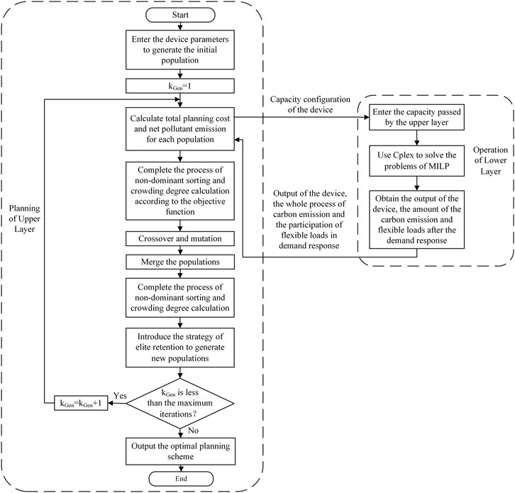
FIGURE 4. Flow chart of solving the double-layer optimization model based on the improved NSGA-II and MILP method.
For further study impacts of the whole carbon emission process and the IDR on the operation and capacity configuration in the system, this paper makes some improvements on the example shown in the work of Wei et al. (2022) and Zeng et al. (2023), and the following four cases are built for comparative analysis:
Case I: The whole process of carbon emission and the IDR involving flexible loads are not considered.
Case II: The whole process of carbon emission is not considered, and the IDR involving flexible loads is considered.
Case III: The whole process of carbon emission is considered, and the IDR involving flexible loads is not considered.
Case IV: The whole process of carbon emission and the IDR involving flexible loads are both considered.
According to the four cases constructed previously, the outcome is enumerated in Table 1.
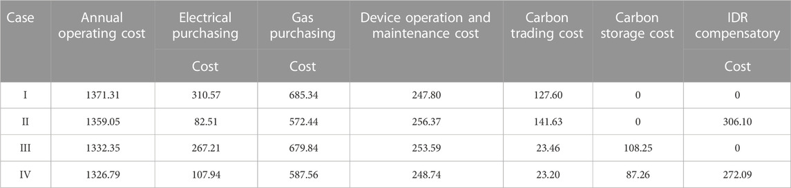
TABLE 1. Cost results of comparative cases within the year (unit: ten thousand Yuan/year).
As shown in Table 1, compared with case I, the costs of carbon trading and annual operating in case III are reduced by 81.61% and 2.84%, respectively. This is because case III considers the whole process of carbon emission and sends the captured CO2 into P2G for carbon utilization, which effectively reduces the net emission of CO2. Moreover, introducing the ladder-type carbon trading mechanism makes the initial carbon quotas offset part of the carbon trading cost, thus reducing the annual operating cost. In addition, compared with case I, the cost of purchasing electricity and gas in case II is reduced by 73.43% and 16.47%, respectively. This is because the process of IDR can significantly cut down the peak-time flexible loads and scale up the valley-time flexible loads, especially the change in the electrical load, which allows the energy purchasing method to be more economical and selective. Compared with case III, the cost of carbon storage in case IV is lower. This is because the electrical load is decreased during peak periods after considering the IDR, which leads to the output power reduction of new energy units. In addition, the reduced part is converted to abandoned wind and light, which increases the amount of CO2 consumed by P2G. Compared with case II, the compensatory cost of IDR in case IV is slightly lower. This is because the peak-to-valley differences of the electrical load are reduced by increasing the on-grid power of new energy units under the combined operation demand, which decreases the compensatory cost of IDR. In addition, the annual operating cost, electricity and gas purchasing cost, device operation and maintenance cost, and carbon trading cost in case IV are all smaller than those in case III, because considering the IDR in the whole process of carbon emission can transfer parts of flexible loads in high-price periods to low-price periods and lower their energy consumption. Moreover, the response process of the mutual substitution involving electricity, heat, and other energy sources also significantly reduces the energy purchasing cost, thus making the operating modes more reasonable, and the economy and the environmental protection tend to be more coordinated in the system.
In addition, compared to case IV, cases I, II, and III have the lowest cost for their respective parts, but the other costs are at a higher level and the overall performance is poor. Case IV has generally lower costs for each subcomponent and has the best overall performance with annual operating cost improvement rates of 3.25%, 2.37%, and 0.42%.
Meanwhile, in an effort to validate the availability and the superiority of the algorithm that is proposed in this paper, quantitative analysis is added on the basis of qualitative analysis to compare the improved NSGA-II with the conventional one. Assuming that the number of populations is 50, the maximum number of iterations is 500, and running each standard test function 30 times, the relevant parameters of test functions (Tao et al., 2019) and the final results including the standard deviation (SD), average fitness (AF), optimal value (OV), worst value (WV), and convergence curve can be obtained as shown in Table 2 and Figure 5.
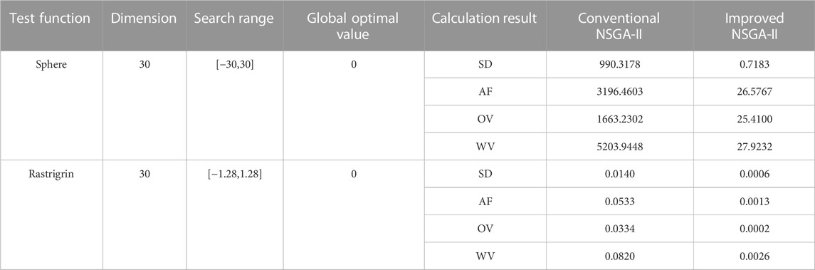
TABLE 2. Relevant parameters of test functions and the calculation results.
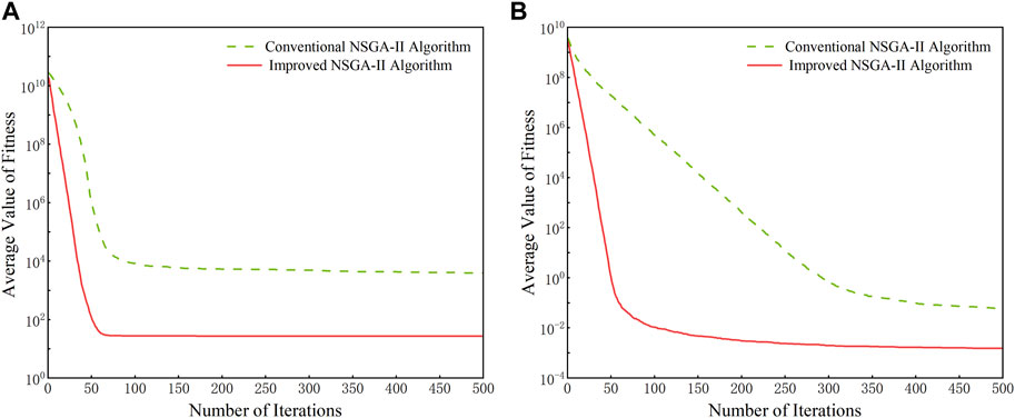
FIGURE 5. Average convergence curve of the test. (A) Results of the function Sphere, and (B) results of the function Rastrigrin.
As is shown in Table 2, both the conventional algorithm and improved NSGA-II can complete the search process, but the improved NSGA-II exhibits higher search accuracy and more divergent data, which indicates the better population diversity. In addition, as shown in Figure 5, the improved NSGA-II is superior to the conventional one in terms of convergence speed, convergence accuracy, global search ability, and optimized stability.
Table 3 shows the configuration of each device obtained by the two algorithms in case IV. As shown in Table 3, capacity configuration results under the improved NSGA-II are generally lower than those under the conventional one, especially for new energy units and storage batteries. This shows that the improved NSGA-II is able to reduce the annual investment cost effectively and then further decrease the annual planning cost of the system, which can diminish approximately 4.03 million Yuan. In addition, the net emission of pollutants is also cut down so that environmental protection can be improved. Main parameters of various types of the devices are listed in Table 4 below.
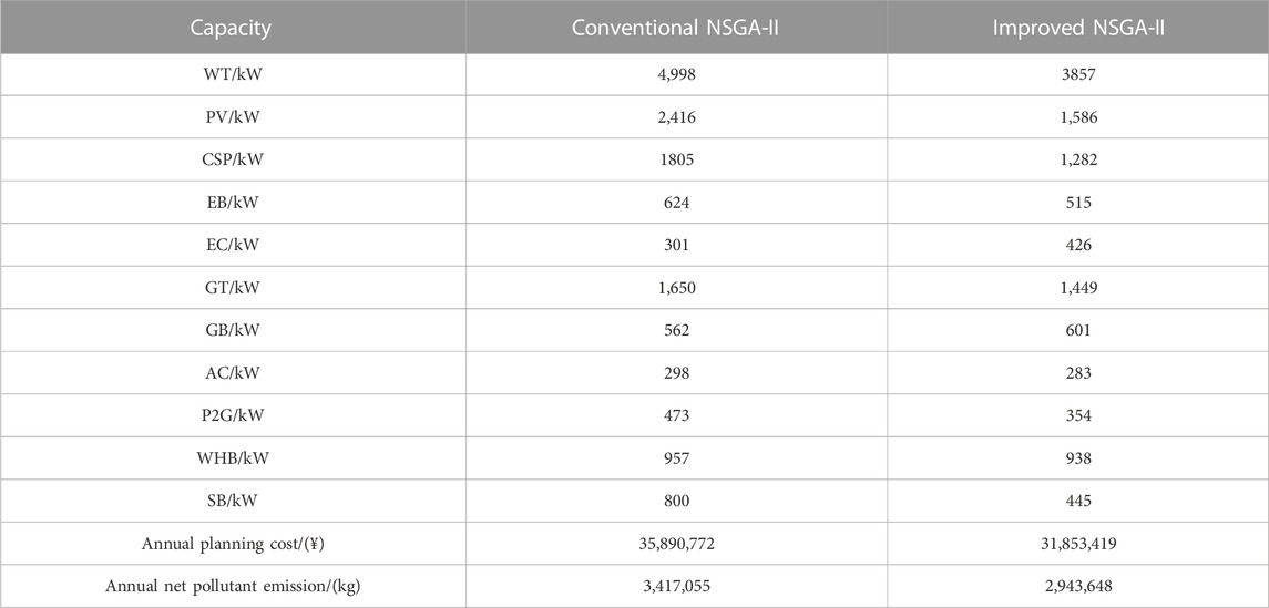
TABLE 3. Configuration results of different algorithms.
TABLE 4. Main parameters of various types of the devices.
This paper takes a typical day in winter to analyze the operating results of the entire RIES. The operating period is 24 h, and the unit operating period is 1 h. The output forecast of renewable energy on a typical winter day is shown in Figure 6. In addition, the corresponding time-of-use price curves are shown in Figure 7.
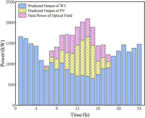
FIGURE 6. Output forecast of renewable energy on a typical winter day in the RIES.
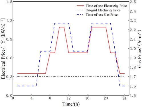
FIGURE 7. Time-of-use price curves.
The situation of carbon emission in different cases is shown in Figure 8, and the flexible load curves such as electricity, heat, cooling, and gas under the IDR as well as their detailed composition in case IV are presented in Figure 9.
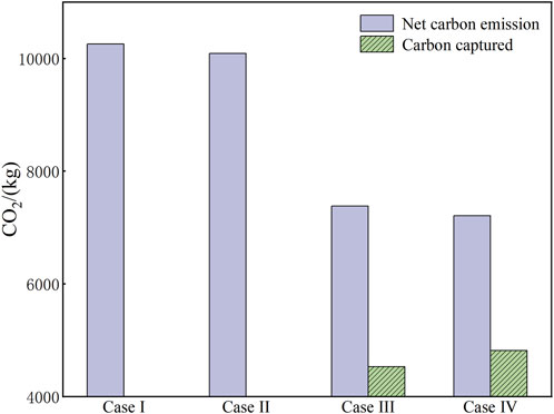
FIGURE 8. Net emission and capture volume of CO2.
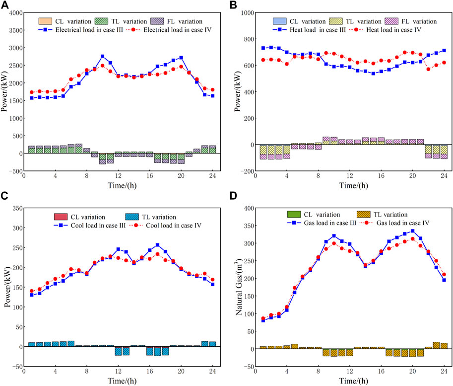
FIGURE 9. Detailed composition of flexible loads. (A) Electrical load, (B) heat load, (C) cool load, and (D) gas load.
As shown in Figure 8, compared with case I and case II, net carbon emissions in case III and case IV are significantly diminished after considering the whole process of carbon emission. Compared with case III, case IV has lower carbon emission and higher carbon capture, which can reduce carbon trading costs to enhance environmental benefits. This is because the IDR of peak cutting and valley filling can reduce some of the purchased power and make the output of new energy units and GTs increase slightly; as a result, the energy consumption of the CCS also increases.
As presented in Figure 9, compared with case III, the CLs, TLs, and FLs of each period in case IV are dynamically changed after considering the IDR, and the maximum peak-to-valley differences of each flexible load are reduced by 36.32%, 35.75%, 26.31%, and 11.42%, thus smoothing the load curves and realizing the process of peak cutting and valley filling. For instance, according to the electrical load in Figure 9A, the variation of CL is reflected in peak periods; the variation of TL is larger in peak and valley periods and smaller in normal periods; and the variation of FL is positive in valley periods and negative in peak and normal periods, which can better reflect the peak and valley characteristics of electricity prices. In addition, the peak-to-valley differences of the flexible electrical load curve in Figure 9A are effectively reduced to make the cost of power purchase continuously decrease. In addition, it is easily known from Figure 9A that the CL of electricity is reflected in peak periods (10:00–11:00 and 17:00–20:00) when the electrical load and price are high, and the reduced load would be converted into incentive subsidies to users. The TL of electricity is shifted from the high-electricity-price periods (10:00–11:00 and 17:00–20:00) to the low-electricity-price periods (23:00–08:00 and 12:00–16:00), which realizes the process of transferring electrical load from peak periods to the valley called peak cutting and valley filling to promote the economy of using the electricity. The FL of electricity converts part of the electrical load into heat load in high electricity price periods to alleviate the mismatch and imbalance between the electrical load demand and the supply capacity. In addition, during the periods of low electricity prices, part of the heat load is transformed into the electrical load for central heating.
The analysis method of the flexible heat load shown in Figure 9B is similar to that of the electrical load. As for the flexible cool and gas loads shown in Figures 9C, D, the system smoothes their load curves by cutting or transferring to realize the process of stabilizing the load fluctuation, which makes the output of the corresponding device more reasonable and perfect.
The aforementioned analysis shows that the IDR under case IV can achieve peak cutting and valley filling to improve economic benefits. Meanwhile, the peak-to-valley differences of each load are reduced by 430.41, 70.60, 33.22 kW, and 29.08 m3 compared with case III, which makes the whole system more flexible in terms of energy purchase so that the environmental benefits are significantly increased.
Figure 10 shows the optimized operation scheme of storage devices involving the storage battery and heat storage tank of the CSP station. Since the energy storage devices can be used as a part of the flexible load, they have abilities to participate in the whole peak-cutting and valley-filling process. For the storage battery, during the valley period of electrical consumption from 23: 00 to 07: 00, the electrical load and price are both lower, so the storage battery charges at this time to cope with the subsequent peak load. During the peak periods of 10: 00–11: 00 and 17: 00–20: 00, the electrical load and price are both higher, so the storage battery discharges to relieve the pressure in the grid. For the CSP heat storage tank, the main thermal source is the heat-conducting medium of the heat absorber in the optical field, so it will be affected by the operation mode of the CSP station in most periods. For example, from 09: 00 to 12: 00, the heat storage tank can provide thermal energy to the load side. In addition, during the period of 13: 00–16: 00, the light is abundant so that the heat storage tank collects heat from the optical field to meet the demand of thermal use in the evening (17: 00–20: 00). During the period of 23: 00–08: 00, the partial output of the electric boiler will flow into the CSP heat storage tank to realize the heat storage backup process.
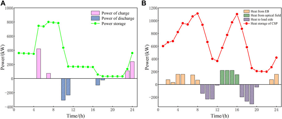
FIGURE 10. Charge/discharge power and the capacity of storage devices. (A) Storage battery and (B) CSP heat storage tank.
The input of the two energy storage equipment makes the operation of the system more reasonable, and the maximum variation range of power storage and heat storage can reach 770 and 911 kW, respectively, which enables the flexibility of energy storage increase significantly to reduce the cost of energy purchase.
Figure 11 shows the optimized operation results of the four energy sources on the typical winter day, which are analyzed as follows:
1) Balance of electricity
As shown in Figure 11A, during the period of 23: 00–05: 00, the electrical demand is mainly satisfied through WT and GT to reduce the costs of electricity generation and device operation. Since the electrical price in this period is at the trough value, the flexible heat load will be converted into electrical load through the IDR, and the system will purchase a small amount of electricity for the storage battery. During the periods of 06: 00–09: 00 and 12: 00–16: 00, the electricity is afforded by WT, PV, CSP station, and GT in priority, and the insufficient part will be supplemented through electrical purchase. During the periods of 10: 00–11: 00 and 17: 00–22: 00, the electrical demands of users are relatively larger. At this time, except for the output of new energy units and GTs, the electrical shortage can be provided by storage battery and electrical purchase, in turn, to maintain the balance. In addition, the participation of flexible electrical load in IDR during this period can further reduce and transfer the peak electricity consumption, thus significantly decreasing the power impact of electrical devices on the grid and their required configuration capacities.
2) Balance of heat
As shown in Figure 11B, during the period of 22: 00–08: 00, the heat is mainly afforded by GB and WHB while the demand is larger than at any other time, so the total amount and the peak value of heat energy can be reduced by cutting and transferring part of the flexible heat load. In addition, due to the low electricity price at this time, a small amount of the heat that is output by EB will be transported to the load side as well as the residual output of EB will flow into the heat storage tank of the CSP station to meet the lower capacity limit. During the period of 09: 00–21: 00, the heat is mainly provided by WHB, and part of the flexible electrical load will be converted into heat load through the IDR. During the period from 09: 00 to 12: 00, as the light gradually increases, the heat storage tank of the CSP station releases the heat to the load side, which reduces the output of GB to 0. During the period from 13: 00 to 16: 00, WHB takes most of the heat load, and the heat storage tank of the CSP station uses this period to charge as the reserve for the next period. During the period from 17: 00 to 21: 00, the gas prices are high so that the output of GB is decreased, and at the same time, the output of electrical generation in the CSP station is continuously reduced; as a result, the heat storage tank of the CSP station releases the heat to the load side. If the demand cannot be satisfied, EB will provide part of the required heat.
3) Balance of cooling
As shown in Figure 11C, the output of EC completes the supply of cool load in the valley and normal time of electrical price, such as the periods of 21: 00–09: 00 and 12: 00–16: 00. During the periods of high electricity price such as 10: 00–11: 00 and 17: 00–19: 00, the output of EC is less than before and AC bears all the cool load, which is helpful for peak cutting and valley filling. Since there is little demand for cool energy in winter, the cool mode of the system is relatively flexible. As a result, the flexible cooling load only needs to be partially reduced and transferred at the peak.
4) Balance of gas
As shown in Figure 11D, the gas load and the consumption of gas-fired units are satisfied through gas purchase during the periods of 22: 00–08: 00 and 13: 00–16: 00. During the period from 22: 00 to 05: 00, although the gas price is at the trough value, the consumption of gas is generally small, and as a result, the gas purchase is still relatively small. During the period from 06: 00 to 08: 00, the gas purchase is growing and GT becomes the main source of gas consumption and continuously increases its output to satisfy the demands of electricity and heat. During the period from 13: 00 to 16: 00, the consumption of the gas-fired units is maintained within a certain range due to the influence of the climbing rate. At this time, the gas load fluctuates slightly but the amplitude is small; therefore, the corresponding gas purchase is basically at a stable level. During the periods of 09: 00–12: 00 and 17: 00–21: 00, constraints on carbon capture and flue gas treatment make regulating abilities of the system decline, which leads to the abandonment of wind and light. At this time, P2G makes efforts to absorb the abandoned power of wind and light, which can synthesize natural gas to alleviate the imbalance between gas purchase and gas demands. Moreover, due to the high gas price in this period, the flexible gas load will be reduced and transferred accordingly.
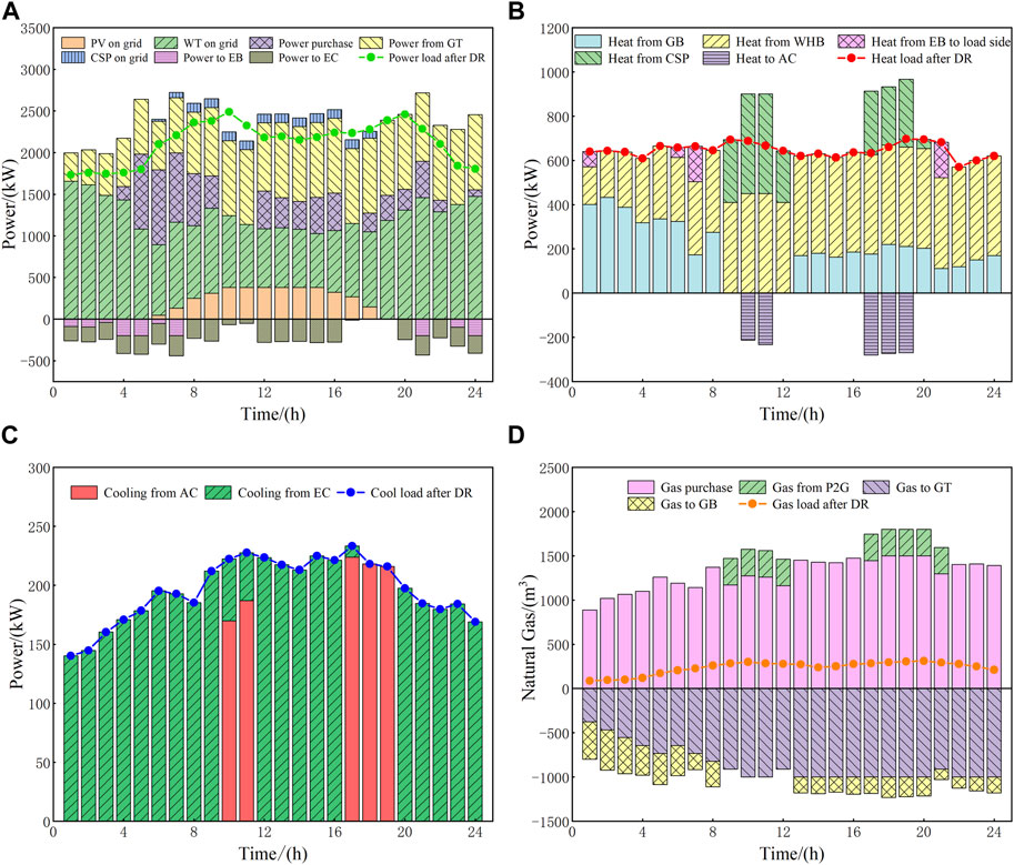
FIGURE 11. Optimal balance scheduling results on a typical winter day. (A) Electrical load, (B) heat load, (C) cool load, and (D) gas load.
In this paper, an operating model of RIES that considers the whole process of carbon emission and IDR is constructed. Meanwhile, a double-layer optimal configuration method based on the improved NSGA-II and MILP is proposed with the participation of the CSP station. The following conclusions can be drawn by setting up four cases:
1) The proposed double-layer optimal configuration model can reasonably optimize the capacities and the output of the devices to obtain the optimal operation scheme. Meanwhile, the participation of the CSP station can improve the coordinated optimization abilities of the RIES.
2) Compared to not considering carbon emissions, introducing the whole process of carbon emission can significantly reduce the net carbon emission, in which the combined operation strategy of wind power–photovoltaic–CSP–carbon capture can coordinate the output of each device and suppress the fluctuation of renewable energy, the process of carbon utilization decreases the storage cost and promotes P2G to absorb the abandoned power of wind and light, and the ladder-type carbon trading mechanism can strictly control the cost of carbon emission to enhance the economy and environmental protection.
3) Compared to not considering IDR, classifying flexible loads including electricity, heat, cooling, and gas into curtailable, transferable, or fungible loads for participating in the IDR can effectively smooth the load curves, reduce the peak-to-valley differences, and realize multi-energy complementarities. Meanwhile, the compensatory mechanism of the IDR can rationally adjust the energy consumption strategies to optimize the energy structure and improve energy efficiency.
4) Compared with the conventional NSGA-II, the improved NSGA-II can obtain the optimal non-dominated solution sets in the upper layer, and its capacity configuration and operation scheme have lower annual planning cost and net pollutant discharge. Meanwhile, the optimized accuracy of the improved NSGA-II is higher, and the convergent speed and ability reach the optimal level.
At present, this paper mainly studies the day-ahead configuration and operation of the single-region RIES. In the follow-up work, the whole process of carbon emission and IDR will be further extended to the energy network with multi-RIES interconnection by considering the effects of source-load uncertainty on capacity configuration and the step-by-step refinement of time scales to realize the decoupling, coordinated optimization, and stable operation of different energies.
The original contributions presented in the study are included in the article/Supplementary Material; further inquiries can be directed to the corresponding author.
XZ: methodology, algorithm finding, and experimental platform provision. JW: programming, simulation, and writing original draft preparation. YZ: algorithm refinement, editing, supervision, and review. HL: raw data provision, algorithm testing, and article refinement. All authors contributed to the article and approved the submitted version.
This work was supported by the National Natural Science Foundation of China (No. 52167014); Small and Medium-sized Enterprise Innovation Fund of Gansu Province (No. 22CX3JA002); and Natural Science Foundation Project of Gansu Province (No. 21JR7RA211).
The authors declare that the research was conducted in the absence of any commercial or financial relationships that could be construed as a potential conflict of interest.
All claims expressed in this article are solely those of the authors and do not necessarily represent those of their affiliated organizations, or those of the publisher, the editors, and the reviewers. Any product that may be evaluated in this article, or claim that may be made by its manufacturer, is not guaranteed or endorsed by the publisher.
Azzam, S. M., Elshabrawy, T., and Ashour, M. (2023). A bi-level framework for supply and demand side energy management in an islanded microgrid. IEEE Trans. Ind. Inf. 191, 220–231. doi:10.1109/tii.2022.3144154
Chen, B., Wu, W., Guo, Q., and Sun, H. (2022). An efficient optimal energy flow model for integrated energy systems based on energy circuit modeling in the frequency domain. Appl. Energy 326, 119923. doi:10.1016/j.apenergy.2022.119923
Chen, W., Ma, Y., and Bai, C. (2021). The impact of carbon emission quota allocation regulations on the investment of low-carbon technology in electric power industry under peak-valley price policy. IEEE Trans. Eng. Manage. early access, 1–18. doi:10.1109/tem.2021.3121002
Dong, W., Lu, Z., He, L., Geng, L., Guo, X., and Zhang, J. (2022). Low-carbon optimal planning of an integrated energy station considering combined power-to-gas and gas-fired units equipped with carbon capture systems. Int. J. Electr. Power & Energy Syst. 138, 107966. doi:10.1016/j.ijepes.2022.107966
Fan, H., Yu, Z., Xia, S., and Li, X. (2021). Review on coordinated planning of source-network-load-storage for integrated energy systems. Front. Energy Res. 9, 641158. doi:10.3389/fenrg.2021.641158
Fu, X., Zeng, G., Zhu, X., Zhao, J., Huang, B., and Liu, J. (2022). Optimal scheduling strategy of grid-connected microgrid with ladder-type carbon trading based on Stackelberg game. Front. Energy Res. 10, 961341. doi:10.3389/fenrg.2022.961341
Gorman, B. T., Lanzarini-Lopes, M., Johnson, N. G., Miller, J. E., and Stechel, E. B. (2021). Techno-economic analysis of a concentrating solar power plant using redox-active metal oxides as heat transfer fluid and storage media. Front. Energy Res. 9, 734288. doi:10.3389/fenrg.2021.734288
Jiang, P., Dong, J., and Huang, H. (2020). Optimal integrated demand response scheduling in regional integrated energy system with concentrating solar power. Appl. Therm. Eng. 166, 114754. doi:10.1016/j.applthermaleng.2019.114754
Li, Y., Bu, F., Gao, J., and Li, G. (2022). Optimal dispatch of low-carbon integrated energy system considering nuclear heating and carbon trading. J. Clean. Prod. 378, 134540. doi:10.1016/j.jclepro.2022.134540
Shao, C., Ding, Y., Siano, P., and Lin, Z. (2019). A framework for incorporating demand response of smart buildings into the integrated heat and electricity energy system. IEEE Trans. Ind. Electron. 662, 1465–1475. doi:10.1109/tie.2017.2784393
Shao, C., Ding, Y., Siano, P., and Song, Y. (2021). Optimal scheduling of the integrated electricity and natural gas systems considering the integrated demand response of energy hubs. IEEE Syst. J. 153, 4545–4553. doi:10.1109/jsyst.2020.3020063
Tao, J., Xu, W., and Li, Y. (2019). Optimal operation of integrated energy system combined cooling heating and power based on multi-objective algorithm. Sci. Tech. Engrg. 19(33), 200–205. doi:10.3969/j.issn.1671-1815.2019.33.029
Wang, B., Sun, H., and Song, X. (2022). Optimal dispatching modeling of regional power-heat-gas interconnection based on multi-type load adjustability. Front. Energy Res. 10, 931890. doi:10.3389/fenrg.2022.931890
Wang, L., Hou, C., Ye, B., Wang, X., Yin, C., and Cong, H. (2021). Optimal operation analysis of integrated community energy system considering the uncertainty of demand response. IEEE Trans. Power Syst. 364, 3681–3691. doi:10.1109/tpwrs.2021.3051720
Wang, X., Xin, A., Chen, X., Fang, L., Jia, Q., Ma, L., et al. (2022). Optimal dispatching of ladder-type carbon trading in integrated energy system with advanced adiabatic compressed air energy storage. Front. Energy Res. 10, 933786. doi:10.3389/fenrg.2022.933786
Wei, Z., Ma, X., Guo, Y., Wei, P., Lu, B., and Zhang, H. (2022). Optimized operation of integrated energy system considering demand response under carbon trading mechanism. Electr. Power Constr. 431, 1–9. doi:10.12204/j.issn.1000-7229.2022.01.001
Yan, M., Li, Y., Chen, G., Zhang, L., Mao, Y., and Ma, C. (2017). A novel flue gas pre-treatment system of post-combustion CO2 capture in coal-fired power plant. Chem. Eng. Res. Des. 128, 331–341. doi:10.1016/j.cherd.2017.10.005
Yan, N., Ma, G., Li, X., and Guerrero, J. M. M. (2023). Low-carbon economic dispatch method for integrated energy system considering seasonal carbon flow dynamic balance. IEEE Trans. Sustain. Energy 141, 576–586. doi:10.1109/tste.2022.3220797
Yang, H., Li, M., Jiang, Z., and Zhang, P. (2020). Multi-time scale optimal scheduling of regional integrated energy systems considering integrated demand response. IEEE Access 8, 5080–5090. doi:10.1109/access.2019.2963463
Zeng, X., Zhang, J., and Wang, X. (2023). Optimal configuration of regional integrated energy system after taking into account multiple uncertainties and the participation of concentrating solar power stations. High. Volt. Eng. 491, 353–363. doi:10.13336/j.1003-6520.hve.20211326
Zhang, D., Yun, Y., Wang, X., He, J., and Dong, H. (2021). Economic dispatch of integrated electricity-heat-gas energy system considering generalized energy storage and concentrating solar power plant. Autom. Electr. Power Syst. 4519, 33–42. doi:10.7500/AEPS20210220002
Zhang, D., Zhu, H., Zhang, H., Goh, H. H., Liu, H., and Wu, T. (2022). Multi-objective optimization for smart integrated energy system considering demand responses and dynamic prices. IEEE Trans. Smart Grid 132, 1100–1112. doi:10.1109/tsg.2021.3128547
Zhang, G., Xie, P., Huang, S., Chen, Z., Du, M., Tang, N., et al. (2021). Modeling and optimization of integrated energy system for renewable power penetration considering carbon and pollutant reduction systems. Front. Energy Res. 9, 767277. doi:10.3389/fenrg.2021.767277
Zhang, N., Hu, Z., Dai, D., Dang, S., Yao, M., and Zhou, Y. (2016). Unit commitment model in smart grid environment considering carbon emissions trading. IEEE Trans. Smart Grid 71, 420–427. doi:10.1109/tsg.2015.2401337
Keywords: regional integrated energy system, concentrating solar power station, NSGA-II, the whole process of carbon emission, integrated demand response
Citation: Zeng X, Wang J, Zhou Y and Li H (2023) Optimal configuration and operation of the regional integrated energy system considering carbon emission and integrated demand response. Front. Energy Res. 11:1218035. doi: 10.3389/fenrg.2023.1218035
Received: 06 May 2023; Accepted: 19 June 2023;
Published: 10 July 2023.
Edited by:
Chengguo Su, Zhengzhou University, ChinaCopyright © 2023 Zeng, Wang, Zhou and Li. This is an open-access article distributed under the terms of the Creative Commons Attribution License (CC BY). The use, distribution or reproduction in other forums is permitted, provided the original author(s) and the copyright owner(s) are credited and that the original publication in this journal is cited, in accordance with accepted academic practice. No use, distribution or reproduction is permitted which does not comply with these terms.
*Correspondence: Yun Zhou, eXVuLnpob3VAc2p0dS5lZHUuY24=
Disclaimer: All claims expressed in this article are solely those of the authors and do not necessarily represent those of their affiliated organizations, or those of the publisher, the editors and the reviewers. Any product that may be evaluated in this article or claim that may be made by its manufacturer is not guaranteed or endorsed by the publisher.
Research integrity at Frontiers
Learn more about the work of our research integrity team to safeguard the quality of each article we publish.