Study of diagnosis for rotating machinery in advanced nuclear reactor based on deep learning model

Many types of rotating mechanical equipment, such as the primary pump, turbine, and fans, are key components of fourth-generation (Gen IV) advanced reactors. Given that these machines operate in challenging environments with high temperatures and liquid metal corrosion, accurate problem identification and health management are essential for keeping these machines in good working order. This study proposes a deep learning (DL)-based intelligent diagnosis model for the rotating machinery used in fast reactors. The diagnosis model is tested by identifying the faults of bearings and gears. Normalization, augmentation, and splitting of data are applied to prepare the datasets for classification of faults. Multiple diagnosis models containing the multi-layer perceptron (MLP), convolutional neural network (CNN), recurrent neural network (RNN), and residual network (RESNET) are compared and investigated with the Case Western Reserve University datasets. An improved Transformer model is proposed, and an enhanced embeddings generator is designed to combine the strengths of the CNN and transformer. The effects of the size of the training samples and the domain of data preprocessing, such as the time domain, frequency domain, time-frequency domain, and wavelet domain, are investigated, and it is found that the time-frequency domain is most effective, and the improved Transformer model is appropriate for the fault diagnosis of rotating mechanical equipment. Because of the low probability of the occurrence of a fault, the imbalanced learning method should be improved in future studies.

1 Introduction

Commercial pressure water reactors (PWRs) are undergoing life extensions from 40 years of operation to 60 years of operation. The safe and economic operation of these plants is considered in anticipation of a second round of license extensions. The technical issues are similar to the life extension of advanced reactors. In fact, many small modular reactors (SMRs) and designed advanced reactors have increased their operating cycles (typically ten more years after the designed 40 years). As key mechanical components both in PWRs and advanced reactors, rotating mechanical equipment unusually operates under harsh environments of elevated temperature, cyclic loading, and even corrosion. Potential flaws could lead to catastrophic incidents with significant financial losses anddeaths; prognostics health management (PHM) has become indispensable to rotating machinery in advanced nuclear reactors. PHM, which is one of the crucial systems in a rotating machine, uses an intelligent diagnosis method as a crucial component to monitor and diagnose issues efficiently (Hamadache et al., 2019). Traditional diagnosis methods mainly apply signal processing methods to identify the features of the recorded signals and then infer possible faults from the identified features (Li et al., 2018; Sun et al., 2018; Zhao et al., 2018). However, signal processing and feature extraction are time consuming and empirical in nature because both operations depend on prior knowledge of the massive and heterogeneous data. Thus, the precise and efficient performance of the diagnosis model is still a challenging problem.

Artificial intelligence-based diagnosis models have recently become a suitable method in many areas, including computer vision (CV), natural language processing (NLP), state diagnosis, and other fields. Typical methods include artificial neural networks (ANN), k-nearest neighbors (KNN), naive Bayes, and deep learning (DL) (LeCun et al., 2015; Liu et al., 2018). Early fault detection techniques for gears, bearings, and rotors were categorized as signal processing techniques and AI-based techniques (Wei et al., 2019). Data-driven health monitoring by DL-based methods has been summarized and tested by Zhao et al. (2019) with regard to monitoring the operation condition of rotating machinery. Duan et al. (2018) reviewed the diagnosis and prognosis of mechanical equipment based on DL algorithms such as the dynamic Bayesian network (DBN) and convolutional neural network (CNN). Lei et al. (2020) performed a comprehensive review of developing intelligent diagnosis models by using machine learning methods. In addition; Ellefsen et al. (2019) introduced and reviewed four well-known DL algorithms—Auto-encoder (AE), CNN, extended short-term memory network (LSTM), and DBN—In practical PHM applications. For smart manufacturing and manufacturing diagnostics, AI-based methods and applications (smart sensors, intelligent manufacturing, PHM, and cyber-physical systems) were also reviewed by Chang et al. (2018).

This article mainly focuses on the deep learning-based diagnosis models of the rotating machinery used in advanced nuclear reactors. An improved Transformer model is proposed, and an enhanced embeddings generator is designed with a CNN-based positional information extractor. A comparison and analysis of the different diagnosis models, including the MLP, CNN, RNN, RESNET, and Transformer, are performed in Section 2. Because nuclear rotating mechanical equipment adapts the vibration signals to diagnose the current status, this article uses the typical healthy bearings datasets from the Case Western Reserve University (CWRU) to train and investigate DL-based diagnosis models. The datasets for the network training and the data preprocessing technique are also introduced in this section. Major findings are presented in Section 3, and a conclusion is drawn in Section 4.

2 Methods and data

Multiple deep learning algorithms are available for constructing diagnosis models. Their features are firstly introduced in Section 2.1. The labeled datasets are crucial for training the neural networks, and the datasets used in the present study are described in Section 2.2. The data processing techniques are introduced in Section 2.3.

2.1 Introduction of DL models

2.1.1 Convolutional neural network

A type of feedforward neural network with deep structure and convolution computing is known as the “convolutional neural network” (CNN). It has been used extensively in image processing and natural language processing since it was initially presented in 1997 (LeCun and Bengio, 1995). The basic components of the CNN include convolutional layers, activation functions, pooling layers, and fully connected layers. This particular type of neural network has demonstrated dominance in image processing (AlexNet won the ImageNet competition in 2012) and classification (ResNet’s accuracy surpassed that of humans in 2016) (He et al., 2016). The RESNET is a deep CNN architecture designed to address the issues of vanishing gradients and degradation in training deep networks. Residual blocks employ skip connections to directly pass the input signal to subsequent layers while learning the residual to represent the change in the network layers. This design allows the model to directly learn the residual, making it easier to optimize the network. In this study, we create five CNN layers for input data and also customize the well-known RESNET (ResNet18) for four different input data types. As a feed-forward neural network with convolution computation and deep design, the convolutional neural network (CNN) is frequently employed in image and natural language processing. A convolutional and pooling layer are included in each hidden layer of a CNN. The convolutional layer converts the local signal of the preceding layer to the ones of the following layer by employing a filter with common weights to derive characteristics from the input signal.

It is challenging to train CNN models with acceptable accuracy of fault diagnosis since the volume of the labeled samples used in fault diagnosis is comparably modest to that of the images in ImageNet. However, deep CNN models can perform well on small data (Yosinski et al., 2014) by combining with transfer learning (Donahue et al., 2014). Since the RESNET may boost accuracy with higher network depth, we transfer the RESNET trained on ImageNet to the fault diagnostic field in this study. The RESNET is naturally applied in the layers of feature extraction to applications for defect diagnosis since it performs well in picture classification and feature extraction.

We have presented a model (Figure 1) that contains four convolutional layers, batch normalization layers, ReLU layers, and a pooling layer for the purpose of fault diagnostics, which is shown in Table 1. Moreover, Table 2 presents the parameters of the RESNET model we used. A three-layered basic block structure with 64, 128, 256, 512, and N neurons, where N is the total number of defect categories, makes up the classification module. The retrieved characteristics are sent into the categorization module.

FIGURE 1

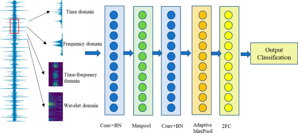
FIGURE 1. Diagramof the CNN model for fault diagnosis of rotating machine.

TABLE 1

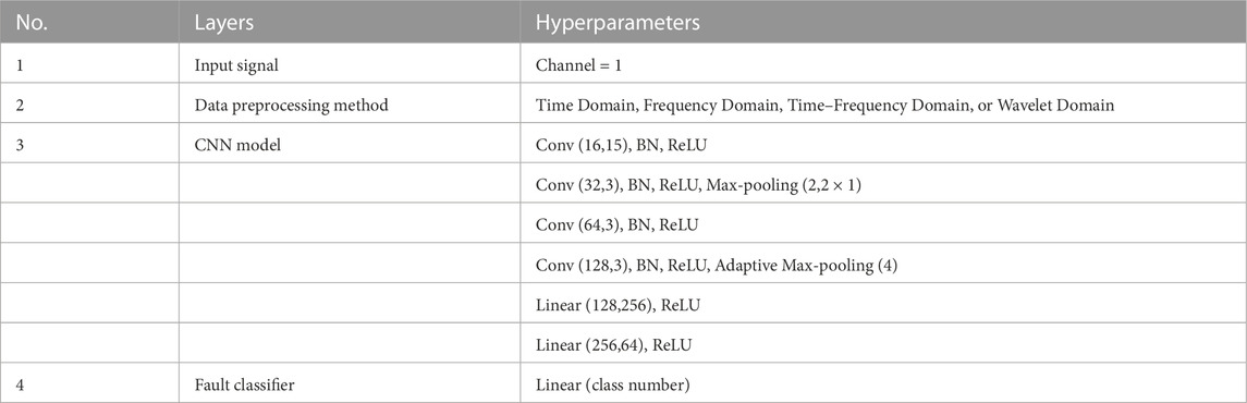
TABLE 1. Parameters of the CNN model.

TABLE 2

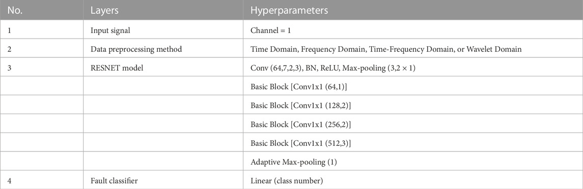
TABLE 2. Parameters of the RESNET model.

2.1.2 Short-term memory network

Due to the CNN’s inability to obtain the long-term dependence characteristics of time series data and the complex features of non-linear data, the RNN is well suited for dealing with time series and has the ability to characterize temporal dynamic behavior. However, there are certain drawbacks to the RNN, such as the potential for gradient explosion or disappearance during backpropagation. For processing continuous input streams, LSTM was introduced in 1997 as a solution to these issues. Bidirectional LSTM (BiLSTM) is able to selectively recall and forget information and can capture bidirectional relationships across extended distances (Hochreiter and Schmidhuber, 1997). For the classification problem, we use BiLSTM to cope with two different forms of input data (Table 3). The RNN is constructed with three layers: the input layer, hidden layer, and output layer. Each layer’s features are represented by the notations $x_t^i$, $h_t^i$, and $o_t^i$, where the superscript and subscript denote the sample number and time step, respectively. U, V, and W are the weight matrix. The forward propagation of a standard RNN is defined as follows:

$h_t^{\left(i\right)}=f\left(w{h}_{t-1}^i+U{x}_t^i+b_u\right)(1)$

$o_t^{\left(i\right)}=v{h}_t^{\left(i\right)}+b_v(2)$

where b_u and b_v are the bias vectors, and f( ) is the non-linear activation function (Gers et al., 2000). The standard RNN is often limited by the long-term dependencies and becomes unable as the sequence grows (Bengio et al., 1994). A common solution is using the architecture of the LSTM network (Figure 2).

TABLE 3

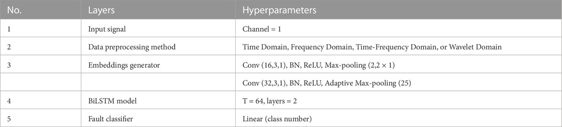
TABLE 3. Parameters of the BiLSTM model.

FIGURE 2

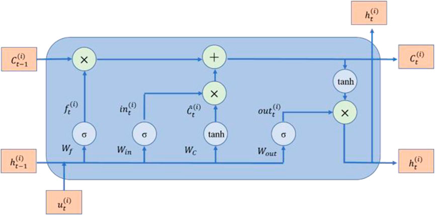
FIGURE 2. LSTM neuron internal structure.

The enhanced classic RNN, or LSTM, can record the entire history of the input data. By combining the forgetting gates, output gates, and input gates, LSTM addresses these issues. The LSTM neuron’s internal organization is depicted in Figure 2. The primary concept is that a number of gates regulate how information flow along the time axis is updated. To decide whether or not the input x_t and hidden state of the preceding layer h(t−1) should be added to the current cell, we introduce the input state. The forget gate controls whether or not the cell value should be preserved in relation to the current input and the prior concealed state. The current layer’s output is based on both the current input and the preceding layer’s output. A set of state responses that incorporate both the most recent input and output data will be produced by LSTM neurons. The memory cell makes sure that the gradient can be transferred to several stages without disappearing or exploding. The update of the input, forget, and output gates is listed as follows:

${\mathit{f}}_t^{\left(i\right)}=\sigma \left[w_f\left(h_{t-1}^{\left(i\right)}+u_t^{\left(i\right)}\right)+b_f\right](3)$

$i{n}_t^{\left(t\right)}=\sigma \left[w_{in}\left(h_{t-1}^{\left(i\right)}+u_t^{\left(i\right)}\right)+b_{in}\right](4)$

$ou{t}_t^{\left(t\right)}=\sigma \left[w_{out}\left(h_{t-1}^{\left(i\right)}+u_t^{\left(i\right)}\right)+b_{out}\right](5)$

$C_t^{\left(i\right)}=\tan h\left[w_c\left(h_{t-1}^{\left(i\right)}+u_t^{\left(i\right)}\right)+b_c\right](6)$

$C_t^{\left(i\right)}=f_t^{\left(i\right)}⚬C_{t-1}^{\left(i\right)}+i{n}_t^{\left(i\right)}⚬C_t^{\left(i\right)}(7)$

$h_t^{\left(i\right)}=ou{t}_t^{\left(i\right)}⚬\tan h\left(C_t^{\left(i\right)}\right)(8)$

where W and V are the input and hidden state weights, respectively, and b stands for the biases. In the t-th update step, the input gate, forget gate, output gate, and cell state are updated by the input x and the hidden state of the (n-1)-th step. The hyperparameters of the BiLSTM model presents in Table 3.

2.1.3 Multi-layer perceptron (MLP)

The MLP, which is a fully connected network with numerous hidden layers, was put forth as the ANN’s model in 1987 (Rumelhart et al., 1985). With such a basic framework, the MLP is capable of performing some basic categorization tasks. However, when the task gets more difficult, the MLP is challenging to train due to the vast number of factors. For the one-dimensional (1D) input data in the current study, an MLP with five fully linked layers and five batch normalization layers is utilized (Table 4). CE loss refers to the softmax cross-entropy loss, BN refers to the batch normalization layer, and FC refers to the fully connected layer.

We use the CNN and MLP neural network topologies in this article. We will assess how well they perform in applications involving fault diagnostics and transfer learning. One-dimensional vibration signals are the type of data used in this work. In this case, a one-dimensional CNN structure is employed. Letx and y represent the neural networks’ input and output vectors, respectively. An input layer, an output layer, and a number of hidden layers make up the MLP. The letter h_i represents the hidden vector. Then, the forward propagation process of the MLP is as follows: where b_i is the bias vector, w_i is the weight matrix, j (×) is the activation function, and softmax(×) represents the softmax classifier. The forward propagation process of the CNN is as follows:

$\begin{array}{ll}\hfill z1& =j\left(x*w1+b1\right)\hfill \\ \hfill c_1& =down\left(z_1\right)\hfill \\ \hfill & \cdots \hfill \\ \hfill zi& =j\left(ci-1*wi+b\mathrm{i}\right)\hfill \\ \hfill \mathrm{c}i& =down\left(\mathrm{z}i\right)\hfill \\ \hfill h1& =j\left(wc1ci=bc1\right)\hfill \\ \hfill y& =softmax\left(wc2h1+bc2\right)\hfill \end{array}(9)$

where down (×) is the pooling operation and * stands for the convolution operation. For both the MLP and CNN, the loss function is a cross-entropy one as follows:

$L\left(y,\widehat{y}\right)=-\frac{1}{n}{{\sum }_i^n{y}_i\log \widehat{y}}_i-\left(1-y_i\right)\log \left(1-{\widehat{y}}_i\right)(10)$

where y_i is one of the labels, ${\widehat{y}}_i$ is one of the predictions, n is the number of the training samples, and n is the number of the batch samples. The training method of both the MLP and CNN is back-propagation (BP) based on the gradient descent strategy. The parameters of the MLP model are shown in Table 4.

TABLE 4

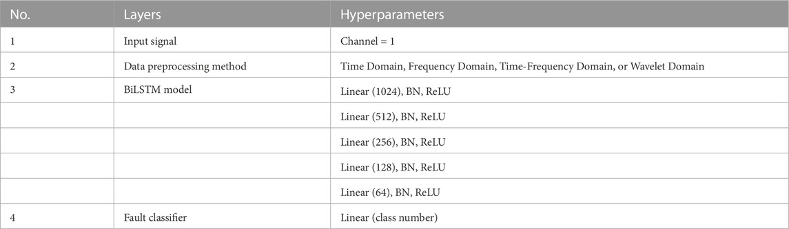
TABLE 4. Parameters of the MLP model.

2.1.4 Improved transformer

Transformer is a deep learning model widely used for natural language processing and other sequence processing tasks. It was developed by Google based on the encoder-decoder framework with an attention mechanism. The Transformer model can handle variable-length sequence data and has better parallelization capability and faster training speed compared to traditional recurrent neural networks (RNNs). The Transformer is composed of multiple stacked encoders and decoders, each consisting of multiple attention sub-layers and fully connected neural network sub-layers. During training, the Transformer uses the self-attention mechanism to capture the relationships between sequences, which effectively handles sequence data.

This study proposes a novel Transformer model for diagnosing faults in rotating machinery by integrating the strengths of the CNN and transformer. The architecture of the proposed model is presented in Figure 3 and consists of three major components: an enhanced embeddings generator, a transformer encoder, and a fault classifier. The parameters of the transformer architecture are listed in Table 5. The enhanced embeddings generator incorporates a CNN-based positional information extractor to convert the preprocessed 1-D data into a sequence of token embeddings. Since the input of the transformer is 1-D sequence tokens, a three-layer 1-D CNN architecture has been designed as an enhanced embeddings generator to ensure that the token embeddings have the same spatial arrangement information as the preprocessed data and that the transformer can access the inductive bias while having local feature extraction ability. The transformer encoder is connected after the input embeddings, which can reduce the model complexity to avoid gradient disappearance during the training process. Because the final output of the transformer is a sequence of the embeddings, an FC layer is used in the fault classifier.

FIGURE 3

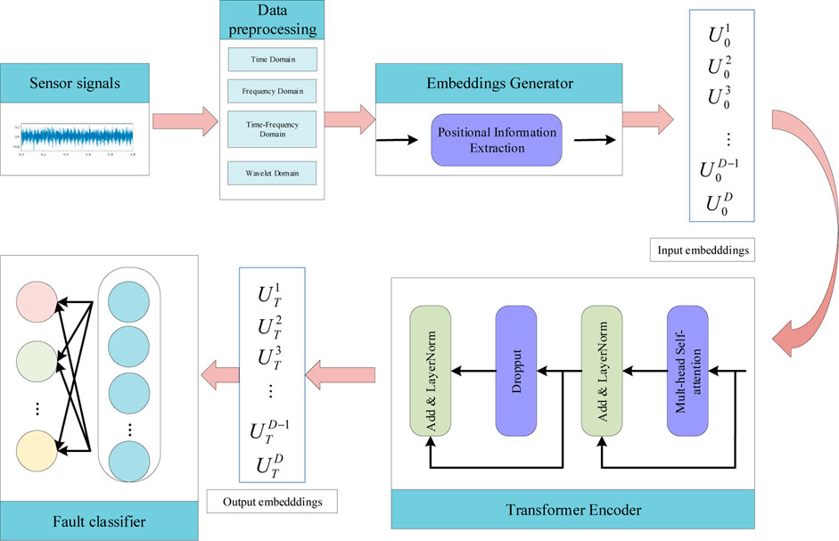
FIGURE 3. Overall architecture of the improved Transformer model.

TABLE 5

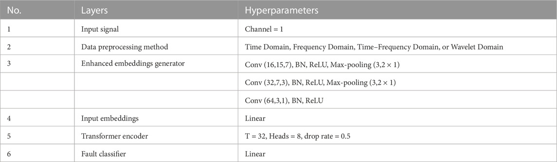
TABLE 5. Parameters of the proposed Transformer model.

2.2 Datasets

Many types of rotating mechanical equipment, such as the primary pump, turbine, and fans, are key components of Gen IV advanced reactors. Normally, industrial vibration detectors are used to monitor and diagnose the rotating machinery state. Although many different failure modes exist in the nuclear industry, the similar fault diagnosis process makes it feasible to investigate the DL-based diagnosis models. We use the typical healthy bearings datasets from CWRU as benchmark testing datasets in order to assess the efficacy of the suggested diagnosis models. Datasets from the Case Western Reserve University (CWRU) have been procured through the Bearing Data Center. Under four different motor loads, vibration signals were recorded at 12 or 48 kHz for healthy bearings and damaged bearings with single-point faults. Single-point defects were added for each operating condition on the rolling element, inner ring, and outer ring, with fault widths of 0.007, 0.014, and 0.021 inches, respectively. The data used in this study were gathered at the drive end, and the sampling frequency employed was 12 kHz.

As shown in Figure 4, the acceleration data were collected both close to and far from the motor bearings. Using electro-discharge machining, defects were introduced into the motor bearings (EDM). The inner raceway, rolling component (the ball), and outer raceway all experienced faults that ranged in dimension from 0.007 inches to 0.040 inches. The test motor’s defective bearings were replaced, and vibration data were collected at loads ranging from 0 to 3 horsepower (the rotating speed ranges from 1797 to 1720 RPM).

FIGURE 4

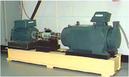
FIGURE 4. Experiment platform for rolling bearing fault sensing.

2.3 Data preprocessing

2.3.1 Time domain

The time domain input denotes the usage of vibration signals without any prior processing as the input. Each sample in this study has a length of 1024. A total of 20% of all the samples are used as the testing set, while 80% of all samples are used as the training set.

2.3.2 Frequency domain

The term “frequency domain” refers to the process of employing the fast Fourier transform (FFT) to convert a sample into the frequency domain. The data length is cut in half as a result of this procedure, and the new sample is described as:

$x_i^{FFT}=\mathit{F}\mathit{F}\mathit{T}\left(x_i\right)(11)$

where the operator FFT(·) represents transforming x_i into the frequency domain and taking the first half of the result.

2.3.3 Time-frequency domain

This kind of input is generated by applying the short-time Fourier transform (STFT) to the samples. The Hanning window is used, and the window length is 64. After this operation, the time–frequency representation (a 33 × 33 image) is generated as:

$x_i^{STFT}=\mathit{S}\mathit{T}\mathit{F}\mathit{T}\left(x_i\right)(12)$

where the operator STFT(·) represents transforming x_i into the time–frequency domain.

2.3.4 Wavelet domain

Continuous wavelet transform (CWT) is used to obtain the wavelet domain representation for the wavelet domain input, as illustrated in Eq. 16 The length of each sample is set at 100 because the CWT requires a lot of time. Following this procedure, the (a 100 × 100 image) wavelet coefficients are produced as:

$x_i^{CWT}=\mathit{C}\mathit{W}\mathit{T}\left(x_i\right)(13)$

where the operator CWT(·) represents transforming x_i into the wavelet domain.

The performance of the DL models is significantly influenced by the type of input data and method of normalization. The complexity of feature extraction is determined by the types of input data, and the difficulty of calculation is determined by normalization techniques and evaluation. This article’s normalizing technique can be used by:

$x_i^{normalize}=\frac{x_i-x_i^{\min }}{x_i^{std}}(14)$

3 Results and discussion

The bearing dataset from the CWRU’s bearing data center have been compared in this study. Four groups of data from the normal bearing, the bearing with the fault on the inner race, the bearing with the defect on the outer race, and the bearing with the fault on the ball make up the dataset. In these tests, four spinning speeds are used, namely, 1797 rpm, 1772 rpm, 1750 rpm, and 1730 rpm. Table 6 contains a list of the label data.

TABLE 6

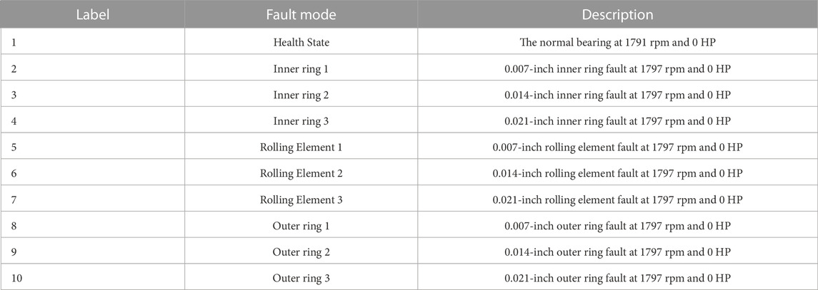
TABLE 6. Label of the modes of fault.

Figure 4 displays the bearing’s vibration signals at a speed of 1797 revolutions per minute. The captured signals were divided into 100 samples, each of which has 1024 points. The testing set and training set can be selected at random. We used 5, 10, 15, and 20 examples of each fault mode for training and the remaining 40 samples for testing in order to compare the performances of the classifiers with various sizes of the training set.

The typical raw vibration signals for ten modes are shown in Figure 5. It is apparent that it is challenging to determine the kind of failure from the raw data without data processing. The time-frequency spectrums with the time-frequency domain and wavelet domain for the ten modes are shown in Figure 6. The proposed diagnosis models have been evaluated against these spectrums.

FIGURE 5

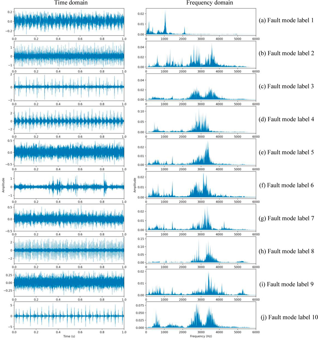
FIGURE 5. Vibration signals in time domain (left) and frequency domain (right) of the 10 fault modes.

FIGURE 6

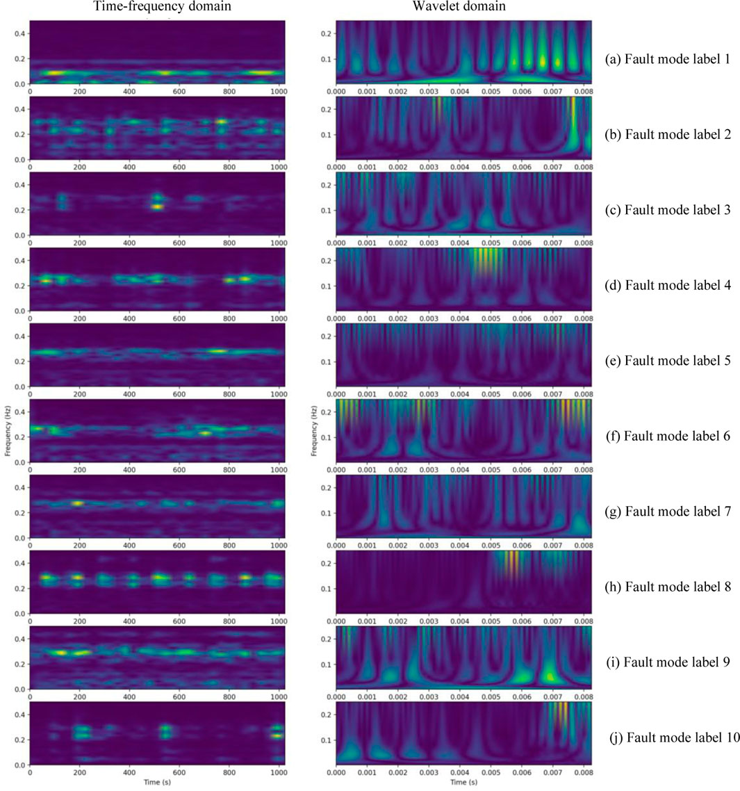
FIGURE 6. The time-frequency spectrum with time-frequency domain (left) and wavelet domain (right) of the 10 fault modes.

As shown in Figure 7, the accuracies of prediction of the CNN, BiLSTM, MPL, RESNET, and Transformer models with different data preprocessing methods are compared. A total of 10 samples are chosen to train the diagnosis models. The CNN, BiLSTM, RESNET, and Transformer models can reach a stable and accurate state after 25 epochs without overfitting. The four data processing techniques are suitable for the three diagnosis models. However, the frequency domain input and time–frequency domain input are appropriate for the MPL as they can achieve the precise model The MPL with the time domain input and wavelet domain input are unable to distinguish the fault modes. In Figure 7, the CNN, BiLSTM, and RESNET have a good accuracy with the time domain and wavelet domain. However, the MLP is unavailable with these two data preprocessing methods. The frequency domain input and time–frequency domain are compatible with these diagnosis models.

FIGURE 7

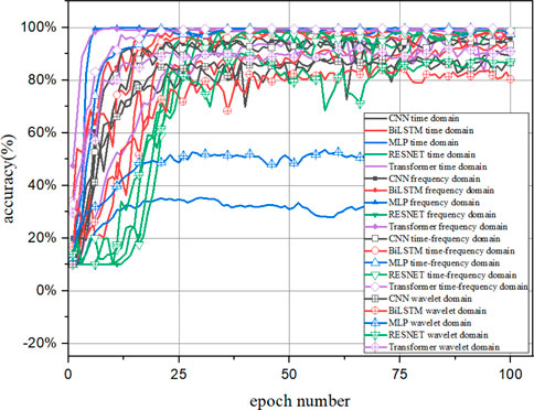
FIGURE 7. The accuracy of the CNN, BiLSTM, MLP, RESNET, and Transformer with epoch number.

In addition to data preprocessing, the train samples number has a great effect on the performance of the diagnosis models (Figure 8). The CNN, BiLSTM, and RESNET methods have a good accuracy with the four data preprocessing methods, with 10 samples for each fault mode. However, the time domain and wavelet domain method show the shortage for the MPL method. The time-frequency domain and frequency method are available for the MPL method, with 5 samples for each fault mode.

FIGURE 8

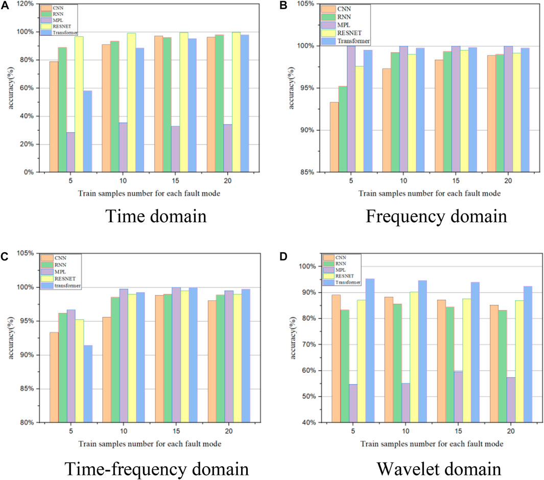
FIGURE 8. The accuracy with the CNN, BiLSTM, MLP, RESNET, and Transformer models with different training sample numbers under different data preprocessing methods: (A) time domain; (B) frequency domain; (C) time-frequency domain; and (D) wavelet domain.

As it is known, signal noise also has great influence on diagnostic accuracy. To test the robustness of the proposed models, white Gaussian noise is added to the training and the testing samples with different signal-to-noise ratios (SNRs). The trend of the different diagnosis models accuracies is shown in Figure 9, with different SNRs using the time-frequency domain input data. For the BiLSTM, MLP, RESNET, and Transformer, the satisfied models are obtained when the SNR is more than 10 dB. The BiSLTM and Transformer show strong anti-noise ability and performs significantly well. Meanwhile, the other models show a shortage in this range of SNR due to overlooking long-term dependencies in the time-series data. BiLSTM models can handle long-term dependencies in time-series data and capture local features in the sequence. Transformer models are based on self-attention mechanisms that effectively handle long-term dependencies between sequence data, which can cause the robustness of the diagnosis model in case of signal noise.

FIGURE 9

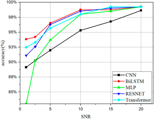
FIGURE 9. The accuracy of the CNN, BiLSTM, MLP, RESNET, and Transformer models with different SNRs.

The key conditions for deep learning diagnosis model processing are sufficient and representative data, proper data preprocessing, and hyperparameter tuning. Deep learning models require sufficient high-quality data to learn and generalize effectively. The dataset should be diverse, balanced, and representative of the various fault types. Sufficient data ensure that the model can capture complex patterns and make accurate predictions. Data preprocessing plays a crucial role in deep learning. It involves tasks such as cleaning, normalization, feature scaling, and handling missing data. Preprocessing ensures that the data are in a suitable format for the model and removes any noise or biases that could hinder learning. Deep learning models have various hyperparameters, such as drop rate, layer number, and regularization parameters, that need to be tuned. Proper hyperparameter tuning can significantly impact the model’s performance, convergence speed, and generalization ability.

4 Conclusion

In the present study, we propose the five DL-based diagnosis models, i.e., the MLP, CNN, RNN, RESNET, and improved Transformer model. The performance of the five models has been evaluated and compared. It is shown that the CNN, BiLSTM, and RESNET can achieve good accuracy of prediction with four types of data preprocessing, even with only 10 samples for training. The MLP method can also yield satisfactory accuracy if the input is provided in the time–frequency domain. The improved Transformer model with the input provided in the time domain and frequency domain is most suitable for the fault diagnosis of rotating machinery.

Data availability statement

The original contributions presented in the study are included in the article/supplementary materials, further inquiries can be directed to the corresponding author.

Author contributions

YS contributed to the conception and design of the study. HW established the fault diagnosis model, organized the database, carried out statistical analysis, and wrote the first draft. YS wrote sections of the manuscript. HW partially revised the manuscript. All authors contributed to the article and approved the submitted version.

Acknowledgments

Thanks are extended to Tsinghua University and Harbin Engineering University for their help in this research.

Conflict of interest

The authors declare that the research was conducted in the absence of any commercial or financial relationships that could be construed as a potential conflict of interest.

Publisher’s note

All claims expressed in this article are solely those of the authors and do not necessarily represent those of their affiliated organizations, or those of the publisher, the editors and the reviewers. Any product that may be evaluated in this article, or claim that may be made by its manufacturer, is not guaranteed or endorsed by the publisher.

References

Bengio, Y., Simard, P., and Frasconi, P. (1994). Learning long-term dependencies with gradient descent is difficult. IEEE Trans. neural Netw.5, 157–166. doi:10.1109/72.279181

PubMed Abstract | CrossRef Full Text | Google Scholar

Chang, C.-W., Lee, H.-W., and Liu, C.-H. (2018). A review of artificial intelligence algorithms used for smart machine tools. Inventions3, 41. doi:10.3390/inventions3030041

CrossRef Full Text | Google Scholar

Donahue, J., Jia, Y., Vinyals, O., Hoffman, J., Zhang, N., Tzeng, E., et al. (2014). Decaf: A deep convolutional activation feature for generic visual recognition. PMLR: International conference on machine learning,647–655.

Google Scholar

Duan, L., Xie, M., Wang, J., and Bai, T. (2018). Deep learning enabled intelligent fault diagnosis: Overview and applications. J. Intelligent Fuzzy Syst.35, 5771–5784. doi:10.3233/jifs-17938

CrossRef Full Text | Google Scholar

Ellefsen, A. L., Æsøy, V., Ushakov, S., and Zhang, H. (2019). A comprehensive survey of prognostics and health management based on deep learning for autonomous ships. IEEE Trans. Reliab.68, 720–740. doi:10.1109/tr.2019.2907402

CrossRef Full Text | Google Scholar

Gers, F. A., Schmidhuber, J., and Cummins, F. (2000). Learning to forget: Continual prediction with LSTM. Neural Comput.12, 2451–2471. doi:10.1162/089976600300015015

PubMed Abstract | CrossRef Full Text | Google Scholar

Hamadache, M., Jung, J. H., Park, J., and Youn, B. D. (2019). A comprehensive review of artificial intelligence-based approaches for rolling element bearing PHM: Shallow and deep learning. JMST Adv.1, 125–151. doi:10.1007/s42791-019-0016-y

CrossRef Full Text | Google Scholar

He, K., Zhang, X., Ren, S., and Sun, J. (2016). Deep residual learning for image recognition. Proc. IEEE Conf. Comput. Vis. pattern Recognit., 770–778. doi:10.1109/CVPR.2016.90

CrossRef Full Text | Google Scholar

Hochreiter, S., and Schmidhuber, J. (1997). Long short-term memory Neural computation. 9, Nov, 15, 8. doi:10.1007/978-3-642-24797-2

CrossRef Full Text | Google Scholar

LeCun, Y., and Bengio, Y. (1995). Convolutional networks for images, speech, and time series. Handb. Brain theory neural Netw.3361, 1995.

Google Scholar

LeCun, Y., Bengio, Y., and Hinton, G. (2015). Deep learning. nature521, 436–444. doi:10.1038/nature14539

PubMed Abstract | CrossRef Full Text | Google Scholar

Lei, Y., Yang, B., Jiang, X., Jia, F., Li, N., and Nandi, A. K. (2020). Applications of machine learning to machine fault diagnosis: A review and roadmap. Mech. Syst. Signal Process.138, 106587. doi:10.1016/j.ymssp.2019.106587

CrossRef Full Text | Google Scholar

Li, C., De Oliveira, J. V., Cerrada, M., Cabrera, D., Sánchez, R. V., and Zurita, G. (2018). A systematic review of fuzzy formalisms for bearing fault diagnosis. IEEE Trans. Fuzzy Syst.27, 1362–1382. doi:10.1109/tfuzz.2018.2878200

CrossRef Full Text | Google Scholar

Liu, R., Yang, B., Zio, E., and Chen, X. (2018). Artificial intelligence for fault diagnosis of rotating machinery: A review. Mech. Syst. Signal Process.108, 33–47. doi:10.1016/j.ymssp.2018.02.016

CrossRef Full Text | Google Scholar

Rumelhart, D. E., Hinton, G. E., and Williams, R. J. (1985). Learning internal representations by error propagation. USA: California Univ San Diego La Jolla Inst for Cognitive Science.

Google Scholar

Sun, C., Ma, M., Zhao, Z., and Chen, X. (2018). Sparse deep stacking network for fault diagnosis of motor. IEEE Trans. Industrial Inf.14, 3261–3270. doi:10.1109/tii.2018.2819674

CrossRef Full Text | Google Scholar

Wei, Y., Li, Y., Xu, M., and Huang, W. (2019). A review of early fault diagnosis approaches and their applications in rotating machinery. Entropy21, 409. doi:10.3390/e21040409

PubMed Abstract | CrossRef Full Text | Google Scholar

Yosinski, J., Clune, J., Bengio, Y., and Lipson, H. (2014). How transferable are features in deep neural networks?Adv. neural Inf. Process. Syst.27, 1.

Google Scholar

Zhao, R., Yan, R., Chen, Z., Mao, K., Wang, P., and Gao, R. X. (2019). Deep learning and its applications to machine health monitoring. Mech. Syst. Signal Process.115, 213–237. doi:10.1016/j.ymssp.2018.05.050

CrossRef Full Text | Google Scholar

Zhao, Z., Wu, S., Qiao, B., Wang, S., and Chen, X. (2018). Enhanced sparse period-group lasso for bearing fault diagnosis. IEEE Trans. Industrial Electron.66, 2143–2153. doi:10.1109/tie.2018.2838070

CrossRef Full Text | Google Scholar