 Wenfa Kang1
 Yajuan Guan1*Fransisco Danang Wijaya2Elias Kondorura Bawan2Adam Priyo Perdana2Juan C. Vasquez1
 Josep M. Guerrero1
- 1AAU Energy, Aalborg University, Aalborg, Denmark
- 2Department of Electrical Engineering and Information Technology, Universitas Gadjah Mada, Yogyakarta, Indonesia
Rural electrification, diesel generator replacement, and resilient electrification systems against natural disasters are among the main targets for Perusahaan Listrik Negara (PLN) in Indonesia to achieve a universally accessible, resilient, and environment-friendly electricity supply. Microgrids, therefore, become a popular and available way to achieve the aforementioned targets due to their flexibility and resiliency. This paper aims to provide a resilience-oriented planning strategy for community microgrids in Lombok Island, Indonesia. A mixed-integer linear program, implemented in the distributed energy resources customer adoption model (DER-CAM), is presented in this paper to find the optimal technology portfolio, placement, capacity, and optimal dispatch in a community microgrid. The multinode model is adopted for the planning, and hence, power flow constraints, N-1 contingency, and technology constraints are considered. The results show that the placement of photovoltaic (PV) arrays, battery energy storage systems (BESSs), and diesel generators (DGs) as backup sources in multi-node community microgrids lead to multiple benefits, including 100% rural electrification, over 25% cost savings, as well as over 22%, in particular CO2 emission reduction in multinode community microgrids.
1 Introduction
Over recent years, about 80% of the world’s primary energy is being provided by fossil fuels, and the energy consumption rate has increased at 2.3% per year from 2015 to 2040, which inevitably increases the CO2 levels in the atmosphere (Martinez-Frias et al., 2008). High level of CO2 in the atmosphere causes the rise of average global temperature, which leads to adverse effects on global climates. Moreover, the burning of fossil fuels to gain electrical energy causes global warming and produces environmental pollutants such as NOx, SOx, and other volatile organic compounds. Therefore, the feasible way to shift to a lower carbon society is to impose carbon taxes and carbon trading polices (Chu et al., 2017).
However, for remote areas without access to the existing electricity grid, locally available resources, such as renewable energy resources (RESs), are promising to support local loads by using microgrid technologies due to their flexibility endowed by advanced control technologies and energy storage systems. In addition, the least cost electrification program in Indonesia is the off-grid generation. In other words, solar battery-basedmicrogrids/min–microgrids are the most suitable and cost-effective options for achieving universal access to electricity (ESCAP, 2020). Furthermore, in some extreme cases, for example, utility black outages or natural disasters, microgrids can work in islanded mode to support the local critical loads and to assist the electricity recovery of adjacent areas, which enables the power distribution network to be more resilient and reliable (Wang and Lu, 2020). Based on the aforementioned arguments, the optimal planning of microgrids is the very first essential step to achieve universal access to electricity, energy transition of Indonesia, and CO2 emission reduction. This is also in line with the government’s commitment to convert conventional power plants to renewable energy generators (PLN, 2021) and Sustainable Development Goals (SDGs) number 7 (IEA and IRENA, 2021).
The optimal portfolio, sizing, and placement of renewable energy resources form a complicated problem because of the features of renewable energy resources; stochastic load demand; and large numbers of continuous and discrete variables, integers, and parameters considered during the design of microgrids. Hence, the optimal planning method can decrease the investment cost with full use of technology components.
Several techno-economic studies have investigated the planning of community microgrids with the RES and energy storage systems (ESSs) (Mizani and Amirnaser, 2009; Hafez and Bhattacharya, 2012; Hittinger et al., 2015; Schittekatte et al., 2016; Madathil et al., 2017; Cao et al., 2019; Borghei and Ghassemi, 2021). Hafez and Bhattacharya (2012); Hittinger et al. (2015) designed microgrid planning models based on the Hybrid Optimization of Multiple Energy Resources (HOMER) software, where life cycle cost and environmental emissions are considered. In Stadler et al. (2013), Stadler et al. (2016), Prathapaneni and Detroja (2019), Borghei and Ghassemi (2021), microgrid planning is modeled into a mixed-integer linear programming (MILP) problem, where binary integers are usually considered to find the locations of various energy carriers. The model of power flow constraints, BESS model, and operation costs in these references are linearized. For the non-linear model of power flow equation, BESS model, and operation costs, Wang et al. (2021), Wu et al. (2023) provide mixed-integer non-linear programming (MINLP) models to solve the proposed problems. These solutions are more accurate than solutions obtained from MILP, but are much more time-consuming.
Aside from providing planning models, several software tools are also designed and compared to analyze the electrical, economical, and environmental performance of microgrids with the RES and ESS, which can be seen in Mendes et al. (2011), Bahramara et al. (2016), Khare et al. (2016), Siddaiah and Saini (2016), Jung and Villaran (2017), Cardoso et al. (2019). Although HOMER is one of the popular software tools, this paper adopts the Distributed Energy Resources Customer Adoption Model (DER-CAM) not only due to the flexible and robust optimization algorithms, hourly time step, and scale considerations but also due to the successful applications with modeling microgrids (Lee et al., 2015; Jung and Villaran, 2017). The DER-CAM tool was designed by Lawrence Berkeley National Laboratory (LBNL) to provide optimal planning and operation of distributed energy generation (DER) either in a distribution system or in microgrids (Stadler et al., 2014). The optimization objective in the DER-CAM contains annual costs and CO2 emissions.
Normally, the key inputs of the model are load profiles, solar radiation, wind speed, water speed, tariff and fuel prices, and user-defined lists of preferred investment of technologies. The outputs of the DER-CAM include optimal portfolios, placements, sizing of DER and ESS, energy dispatch, CO2 emissions, and fuel consumption. With the development, the DER-CAM tool has two basic models, namely, single node and multi-node planning model. In the multi-node planning model, the power flow constraints are integrated. In addition, N-1 contingency and ancillary services are considered (Cardoso et al., 2017; MadathilChalil et al., 2017; Mashayekh et al., 2018). The contribution of this work lines in the modeling of multi-node community microgrids for the Lombok Island based on the native practical data, also in providing strategies for rural electrification in Indonesia. Compared with the HOMER-based strategies, the provided strategy includes the power line flow in the planning. In addition, the sensitivity analysis demonstrates that the proposed planning model is robust to capital cost variations.
This paper presents a technique for optimal planning and operation of microgrids with the RES and ESS in the multi-node model in the context of Lombok Island, Indonesia. The rest of the paper is organized as follows. Section 2 introduces the model of a multi-node microgrid. Section 3 proposes the planning objectives and constraints for community microgrids. Data inputs and parameter setup are presented in Section 4. Section 5 introduces the planning results for multi-node (networked) microgrids. The conclusion of the paper is presented in Section 6.
2 The model of community microgrids
Figure 1 shows the model of a multi-node microgrid. The microgrid has two operation modes—islanded mode and grid-connected mode. Each node is composed of various loads, including electricity loads (household electricity equipment, air conditioner, washing machine, and refrigerator). The objective function of planning is to determine the capacity and placement of various DER technologies with minimized cost and carbon dioxide (CO2) emissions subject to constraints such as capacity constraints and operation constraints (electricity and thermal) of various technologies.
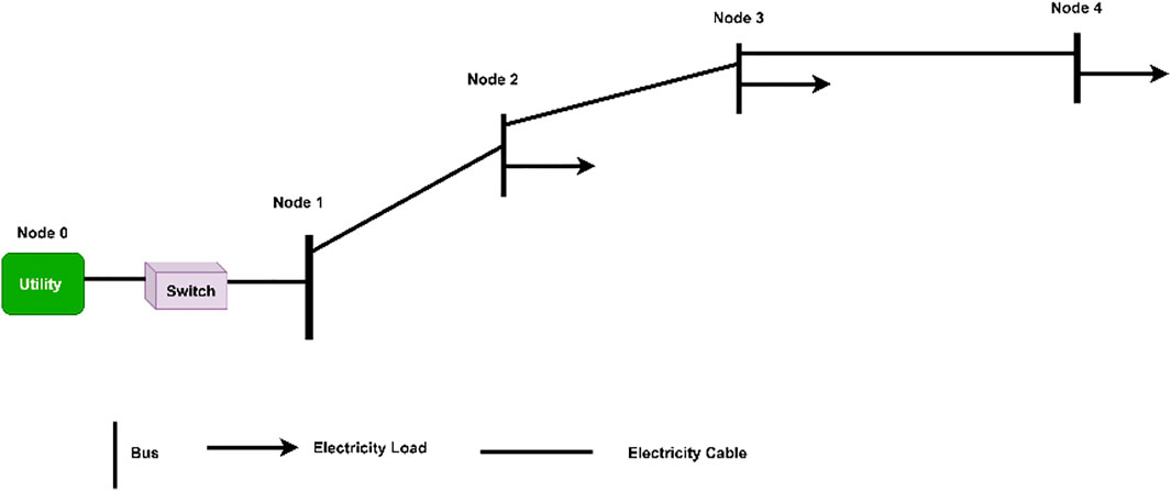
FIGURE 1. Multi-node community microgrids.
3 Planning model of community microgrid headings
3.1 Objective function
Three typical load profiles are adopted in the planning, namely, weekday profile, weekend day profile, and peak day profile. For a typical year characterized by the three load profiles, the time step equals the Number of Months × Hours × Types of load profile, which is 12 × 24 × 3 = 864.
The objective function of planning is to minimize the overall microgrid investment and operation cost including emission cost in the typical year aforementioned. The objective function is formulated as follows (Eq. 1):
where CInv is the annualized investment cost of various technologies, CPur is the total cost of electricity purchase with CO2 taxation, CDe is the demand charge fee, CEx is the electricity export revenue, CG is the generation cost of various technologies including variable maintenance costs, CFM is the fixed maintenance cost, CCO2 is the CO2 taxation on local generations, and CCur is the load curtailment costs.
The annualized investment cost, including the capital cost of discrete technology (Diesel Generator, DG) and capital cost of continuous technology (BESS and PV), is formulated as follows:
where Invn,g is the integer units of discrete generation technology g at node n, PRate,g is the power rating of discrete generation technology g (kW), and CTurn,g is the turnkey capital cost of discrete generation technology g ($/kW). CFX,k is the fixed capital cost of continuous technology k ($), Cvar,k is the variable capital cost of continuous technology k ($/kW), Purn,k is the binary installation decision for continuous technology k, Capn,k is the installed capacity of continuous technology k at node n, and rAnn,i is the annuity rate for the technology i at node n. As observed, the investment costs are decided by the investment decisions of technology, which are Invn,g, Purn,k and the installed capacity Capn,k.
The purchase cost of microgrids is shown in (Eq. 3)
where Pgt is the utility electricity purchasing price at time t, CTax is the tax on CO2 emissions, MCRTt is the marginal carbon emissions from marketplace generation, and Putn,t is the electricity purchased from the utility.
The demand charge cost is as follows:
where DRtm,p is the power demand charge for month m and period p, ($/kW) and MPurn,m,p is the maximal electricity purchased from the utility during period p of month m at node n.
The electricity export revenues are as follows:
where ExRtt is the energy rate for electricity export ($/kWh) and ExPn,t is the electricity exported to the utility at node n.
where Genn,j,t is the output of technology j to meet energy use u at node n and GCstj and Mvar,j are the generation cost of technology j ($/kWh) and variable annual operation and maintenance cost of technology j ($/kWh), respectively.
where MFg is the fixed annual operation and maintenance cost of technology g, $/kW capacity.
In addition, the carbon taxation on local generation is formulated as follows:
where GCRtj is the carbon emission rate from generation technology j (kg/kWh) and ηj is the electrical efficiency of generation technology j.
where PLcurn,u,t is the customer load not met in energy consumption u at node n (kW) and CurPrn,u is the load curtailment cost for energy use u at node n ($/kWh).
As described in Eqs 2–9, the total cost objective function includes 1) annualized investment costs of discrete and continuous technologies; 2) total cost of electricity purchase inclusive of carbon taxation; 3) demand charges; 4) electricity export revenues; 5) generation cost for electrical, heating, or cooling technologies inclusive of their variable maintenance costs; 6) fixed maintenance cost of discrete and continuous technologies; 7) carbon taxation on local generation; and 8) load curtailment costs. The optimization variables include X = [Invn,g, Purn,k, Capn,k, Putn,t, MPurn,m,p, ExPn,t, Genn,j,t, and PLcurn,u,t], which are composed of continuous and binary variables. Parameter Y = [ PRate,g, CTurn,g, CFX,k, Cvar,k, rAnn,i, Pgt, CTax, MCRTt, DRtm,p, ExRtt, GCstj, MFg, GCRtj, ηj, and CurPrn,u] is the constant associated with the planning, which should be determined before solving the optimization objective.
The constraints include energy balance constraints, power flow constraints, storage constraints, cable current constraints, and energy import/export constraints.
The power flow constraints include current and voltage constraints for multi-node microgrids. However, for single-node microgrids, power flow constraints can be ignored. In this paper, a linear power flow model is considered for a balanced multi-node microgrid. It is assumed that the slack bus of microgrids is denoted by N, which means that the voltage of node N is
3.2 Electricity balance constraints
The power flow is represented as follows:
where active power outputs from node n Pgn,t are related to the exported/imported power to/from the utility, power generated from the installed energy resources (PV, DG, FC, and WT), load demand and curtailed loads, consumed power by electric chiller, and the discharged/charged power from energy storage systems. Parameter co1 is the coefficient of the electric chiller, and ηdis/ηch is the discharge/charge efficiency of BESSs. Moreover, each node has the constant power factor ϕ. The nodal voltages Vn,t shown in Eqs 11, 12 are calculated by the nodal active/reactive power injection and network impedance matrix Z without the slack bus row and column. Equation 13 is the power loss of the network, which is used to decide the placements of DERs. In addition, rn,n′ and xn,n′ are the resistance and inductance of line impedance between nodes n and n′, respectively; eIrn,n′t and eIin,n′t are the linearized real current Ir2 and image current Ii2 of line (n, n′) (Mashayekh et al., 2017), respectively; and reVn,t and ImVn,t are the real and imaginary part of the voltage amplitude of node n at time t, respectively.
3.3 Operational constraints
The operation constraints contain the nodal voltage constraints, generation capacity constraints, storage constraints, and energy import/export constraints. The constraints of energy storage are formulated as follows:
The generation constraints are formulated as follows
where ηeff is the solar radiation conversion efficiency of generation technology c ϵ (PV, ST), Solart is the average fraction of maximum solar insolation received during time t (%), and Purn,k is the binary purchase decision for continuous technology k at node n. M is a very large positive constant which decides the upper limits of the capacity of the continuous technology. Genn,g,t is the DG power generation of node n at time t. Genn,c,t is the power generation of continuous technology of node n at time t. Capn,k is the capacity of technology k of node n.
For the gird-connected mode, microgrids may import or export energy from/to the utility by the point of common coupling (PCC) node. However, the energy transferred by the PCC node is normally limited, which is as follows:
where psbn,t is the binary electricity purchase/sell decision at node n, M is the maximal energy purchased from the utility, and mExP is the maximal energy exported to the grid.
4 Planning configuration
4.1 Diagram of community microgrid planning
The planning model of community microgrids is described by Eqs 1–16, where the total investment cost, operation cost, emission cost, energy balance, and operation constraints are introduced. The aforementioned optimization problem is a mixed-integer linear optimization problem, which is an NP-hard problem, but can be solved by mature optimization solvers such as Gurobi and Cplex. Before solving the planning problem, one should first initialize the parameters of the problem, such as to define the value of vector Y = [PRate,g, CTurn,g, CFX,k, Cvar,k, rAnn,i, Pgt, CTax, MCRTt, DRtm,p, ExRtt, GCstj, MFg, GCRtj, ηj, and CurPrn,u] according to the demand, energy policy, specific technologies, and tariffs.
Second, the basic load profile of the microgrids should be collected and input into the optimization problem. In addition, solar radiations and wind speed data should also be collected for the planning. Then, with the given parameters and data input, the proposed optimization problem can be solved. In addition, the optimization variables X = [Invn,g, Purn,k, Capn,k, Putn,t, MPurn,m,p, ExPn,t, Genn,j,t, and PLcurn,u,t] will be obtained. Finally, with the optimal solutions, the capacities and placements of energy resources will be given. The diagram of the planning of community microgrids is illustrated in Figure 2.
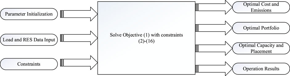
FIGURE 2. Diagram of the planning of community microgrids.
4.1 Data input
The basic data needed for the planning include the load demand for peak day, solar radiations, and electricity rates. The yearly load profiles for nodes 2, 3, and 4 are shown in Figures 3A–C, which are based on the real measured load profile of community microgrids (MGs) in Lombok, Indonesia. Figure 3 shows that the load demand varies from about 200–550 kW from 0 h to 24th hour for node 2. In addition, the load valley is around noon. For node 3, the load peak appears at 18:00, reaching 430 kW for node 3, and the load valley is about 180 kW. For village 1, the load peak comes at 18–19:00, reaching 330 kW. These load profiles are obtained by transferring the practical 5-min loads into a yearly load profile using the DER-CAM. It can be seen the maximal load deviation among months is larger than 100 kW for each node. However, the basic load profiles are similar because Indonesia’s climate is almost entirely tropical, and the temperatures do not vary much from season to season.
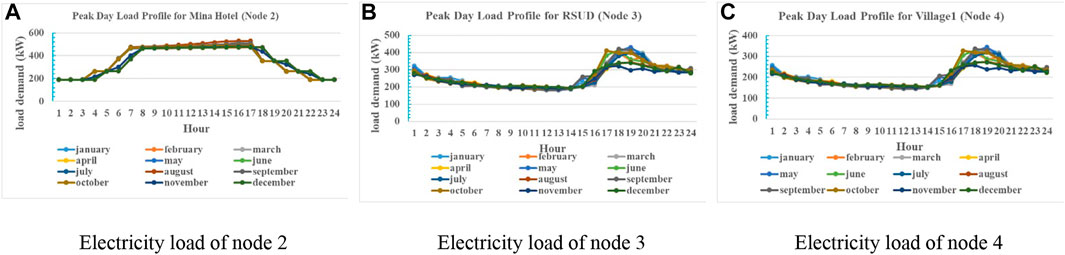
FIGURE 3. Load profiles of community microgrids in 2020. (A) Electricity load of node 2, (B) electricity load of node 3, and (C) electricity load of node 4.
The solar radiation data of Lombok (Indonesia) Island are obtained from the photovoltaic geographical information system. The solar radiation is shown in Figure 4A, from which it can be observed that the maximal power generated is about 0.68 kW/m2. Generally, the PV power output is higher in summer days than in winter days. The electricity price of community microgrids, estimated by the real price in Indonesia, is shown in Figure 4B, where the peak price is 0.4 $/kWh and off-peak price is 0.11 $/kWh. The hours of Time of Use (ToU) rates for summer days are from 12:00 to 18:00 during a day. The PV power sale price is the same as the purchase price in the planning parameter setup.
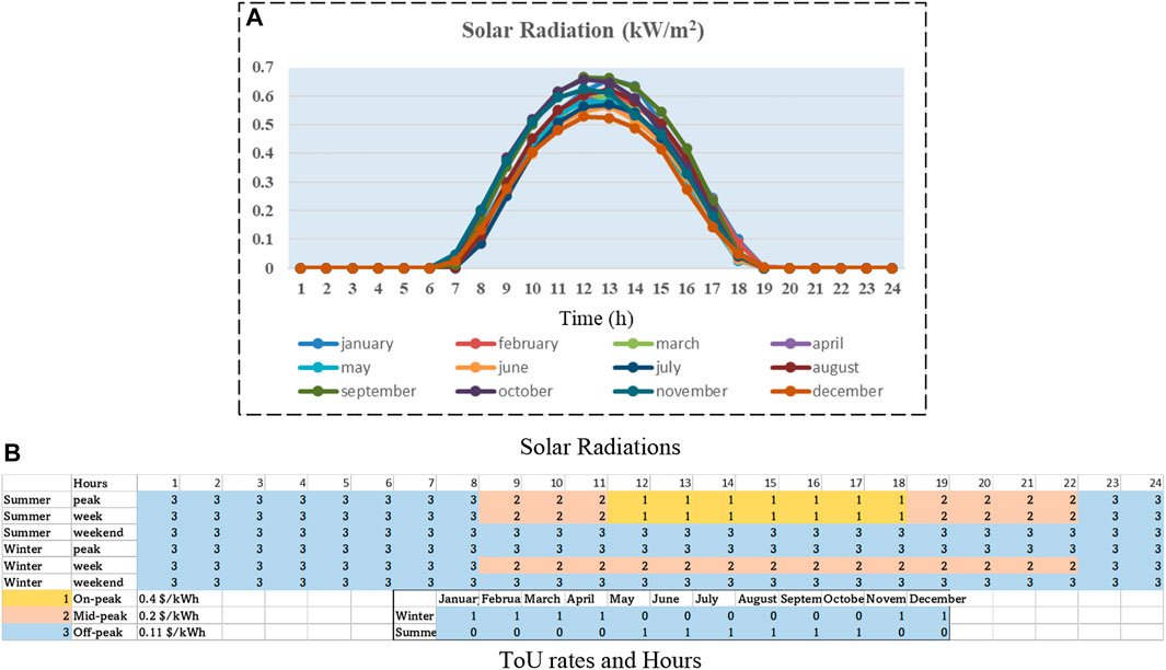
FIGURE 4. PV radiations and Time-of-Use (ToU) rates for community microgrids. (A) Solar radiations and (B) ToU rates and hours.
4.2 System parameters
For the single-node case, the power flow equation is not considered; therefore, the corresponding constraints, such as current constraints and voltage constraints, are neglected in the planning. However, for multiple-node microgrids, the power constraints need to be considered. The planning objectives contain cost minimization and CO2 emission reduction with the same weights, namely, equal to 0.5. The discount rate is set as 3%, and the maximal payback period of microgrids is 20 years. The voltage level is 12 kV, and the maximal capacity of the transformer connected to the upper grid is set as 5 MVA.
The investment cost of PV systems includes fixed investment cost, variable cost, maintenance cost, and inverter cost. In this work, the fixed cost is 2,500 $, and the variable cost is 2,500 $/kW. The lifetime is assumed to be 30 years, and the maintenance cost is 0.005 $/(kW × month). The inverter cost is 500 $/kW-cap for an inverter with a capacity of 100 kW. The investment cost of the BESS includes the fixed cost, variable cost, maintenance cost, and inverter cost. The investment cost is estimated according to the following equation: Investment Cost = (FixedCost + VariableCost × Capacity) × Investment Decision. In this study, the fixed cost is set as 500 $, variable cost is set as 300 $/kW-cap, and variable maintenance cost is set as 0.005 $/(kW × month). The inverter cost of the BESS is set as 200 $/kW-cap for the 100 kVA capacity. The lifetime of the BESS is set as 15 years, while the lifetime of the inverter is 20 years. The battery degradation parameters are shown in Table 1. The cost of diesel generators includes the variable cost and maintenance cost. The variable cost is set as 5761.4074 $/kW. The variable maintenance cost is set as 0.0128 $/kWh, which is dependent on its energy production. Its maximal capacity is 75 kW, with efficiency 0.0238. The other two kinds of DGs are listed in Table 2. The NoXRate is 0.0001 kgNOx/kWh, where NOx emissions are resulted from fuel usage. Its maximum ramp up and ramp down rate is 0.5. The starting time is 20 min, and the time needed to ramp up the generation facility to full capacity is 10 min, which are default parameters in DER-CAM software (Phase, 2018; Heleno et al., 2017).

TABLE 1. Parameters of battery energy storage systems (lithium-ion batteries).
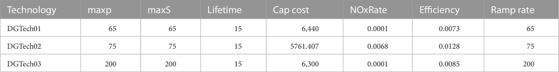
TABLE 2. Unit of items such as maxp (kW), lifetime (year), efficiency (%), and ramp rate (%).
The utility outages contain scheduled outages for scheduled maintenance and unscheduled outages caused by natural disasters or faults. The scheduled outage is defined to occur on the peak day of June of each year, and its duration is 24 h. The unscheduled outage is assumed to occur on the weekdays of December for 24 h. There are three types of loads for load shedding. The first type is low critical loads, which can be cut down for 20% of total loads for 24 h with the cost 0.15 $/kWh. The second type is the middle critical load. In the planning part, middle critical and high critical loads are not chosen to be cut down. The costs of curtailing load are shown in Table 3.

TABLE 3. Costs of load-shedding for the multi-node microgrids.
5 Planning of multi-node networked microgrids
5.1 Costs and capacities
This case study focuses on the multi-node community MG, in which the topology constraints, namely, the power flow equations, are considered. In this case, the community MG has four nodes. Node 1 is Tanjung station, node 2 is Mina Hotel, node 3 is RSUD (hospital), and node 4 is a village nearby. The topology of this community MG is shown in Figure 5, Figure 5A shows the topology in the DER-CAM, and Figure 5B shows the geographical positions of various nodes.
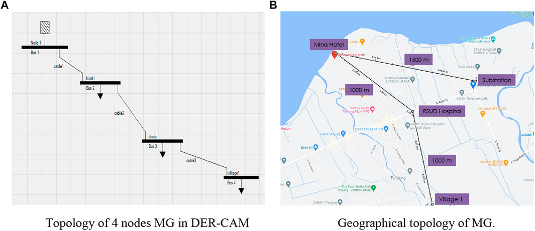
FIGURE 5. Topology of the four-node community microgrid (MG). (A) Topology of four-node MG in the DER-CAM and (B) geographical topology of the MG.
This case study aims to investigate the capacities and locations of DER for the four-node community MG. The main procedure of this planning work is similar with that of the single-node community MG. The difference between the single-node MG and the multi-node MG planning is that in the multi-node MG planning, the power flow equations and the constraints of voltage and current magnitudes should be considered. During the planning, the N-1 contingency is also considered.
The utility outages for multi-node MG include scheduled outages for scheduled maintenance and unscheduled outages caused by natural disasters or faults. The scheduled outage is defined to occur on the weekdays of July of each year. Its duration is 24 h. In addition, the unscheduled outage occurs on the weekends of December for 24 h. There are three types of loads for load shedding in the DER-CAM. The first type is low critical loads, which can be cut down by 20% of the total consumption for 24 h and the cost is 0.15 $/kWh. The second type is the middle critical load. In the planning part, middle critical and high critical loads are not chosen to be cut down.
With the input data and system setup, the planning results can be obtained with the optimized capacities and locations of various energy sources, costs and revenues, and CO2 emissions. Table 4 shows the costs of four-node community MG. With the installation of the PV, DG, and BESS, the total annual energy cost for the MG is 789 k$, which means that the MG earns money by selling energy to the utility each year. Compared with the original case (reference case), the total savings are 22.12%. The CO2 emissions decreased to 1,420 tons per year, with a reduction rate of 25.25%.

TABLE 4. Planning results of multi-node MG.
The optimal placement and combination of technologies are shown in Figure 6A, where node 2 installs two kinds of DG with capacities being 130 and 150 kW, respectively, and one PV with 120 kW capacity, as well as a BESS with 4,539 kWh. For node 3,two DGs with capacities being 65 and 75 kW and 180 kW PV and 3,581 kWh BESS are installed, respectively. Meanwhile, for node 4, only a PV with capacity 748 kW is installed. In the planning, the area constraints for installing PV panels are considered for each node,which are, respectively, 800, 1,200, and 5,000 m2. Therefore, node 2 connects only 120 kW PV. The capital and annualized investment costs of two kinds of DGs are shown in Figure 6B for various capacities.
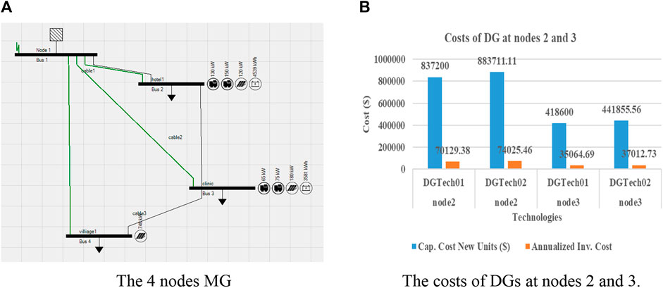
FIGURE 6. Four-node community MG with installed PV and BESS. (A) Four-node MG and (B) costs of DGs at nodes 2 and 3.
5.2 Energy dispatch
The electricity dispatch in July of each year is obtained in Figure 7, where on a peak day, the surplus PV power is exported to the utility, as shown by a gray curve in Figure 7A. In addition, the BESS also discharges during the daylight, shown by dark red area, and during the nights, the BESS is charged by the utility, shown by blue areas. Because during the daylight (from 12:00 to 18:00), the utility price is using on-peak price, shown in Figure 4B, PV sells power to the utility to gain the revenue. In addition, the BESS discharges for local load consumption and during the night, when electricity price is low, the BESS purchases power from utility. During utility outages, the PV and BESS can also provide electricity to the local consumers, as shown in Figure 7B. At most 20% of low critical loads are curtailed in order to keep the system power balance during the utility outages, shown by a red curve.
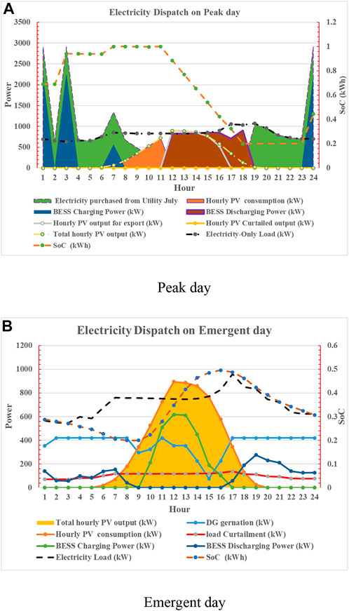
FIGURE 7. Electricity dispatch of the four-node community MG (July). (A) Peak day and (B) emergent day.
For the electricity power interaction among nodes in July on the emergent day, the results are shown in Figure 8. From Figure 8A, it can be observed that the DGs at nodes 2 and 3 start generating power to the MG during the utility outages, where the maximal DG output power at nodes 2 and 3 is 280 and 130 kW, and the minimal output power at nodes 2 and 3 is 75 and 0 kW, respectively. The low critical loads at nodes 2 and 4 also curtail their demand during the outages. The maximal curtailed power of nodes 2 and 4 is 95 and 43 kW, respectively, shown in Figure 8B. The PV outputs and load demands are shown in Figure 8C, where PV power outputs are all consumed by local loads. The BESSs at nodes 2 and 3 provide power to the MG when the PV radiation is low (nights) and absorb power from the MG when the PV output power is high, which is shown in Figure 8D.
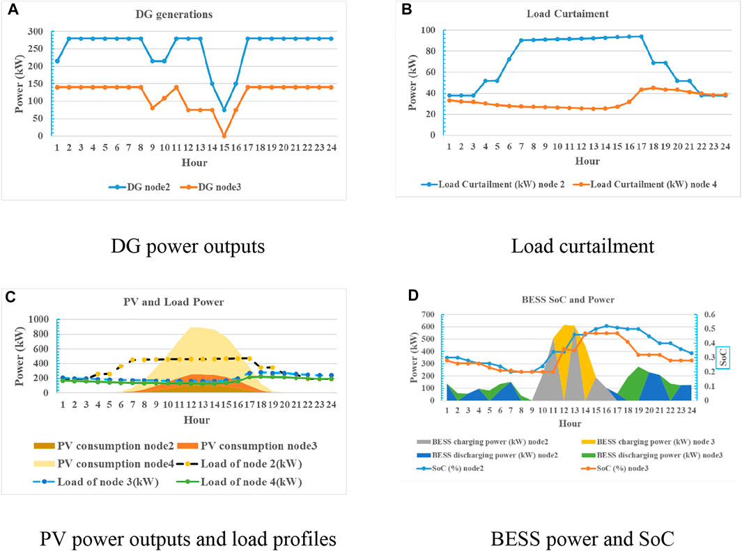
FIGURE 8. Electricity dispatch for each node in the four-node community MG. (A) DG power outputs, (B) load curtailment, (C) PV power outputs and load profiles, and (D) BESS power and SoC.
Figure 9A shows the electricity purchased from the utility during the normal operation, where the peak electricity purchase happens in October and that of valley electricity in March. The difference between peak and valley value is 180,703 kWh. In summer days, solar radiation is high such that the peak PV power is in May, reaching 230,534 kWh/month, while the valley PV power is in February in winter days, shown in Figure 9B. Accordingly, as shown in Figure 9C, during summer days, the PV sources sell power to the utility according to the ToU price illustrated in Figure 4.
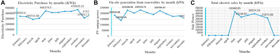
FIGURE 9. Electricity in the four-node MG. (A) Monthly electricity purchase from the utility; (B) monthly PV generation; (C) monthly electricity sales from PV generation.
The nodal voltages of community MG during the utility outages are shown in Figure 10A. With the power flow constraints, the nodal voltages are all varying in the normal range, i.e., [0.95 1.05] p.u., even with the fluctuation of PV power generation and outages. In the planning, node 2 becomes the slack bus providing voltage support. However, during the peak day, the nodal voltages are varying in the normal time, most of the time, except in conditions of heavy load demand. However, the nodal voltages are very close to the lower voltage limit. In the planning, only the active power dispatch is considered, and the voltage will be recovered into the normal range if reactive power dispatch is taken into account.
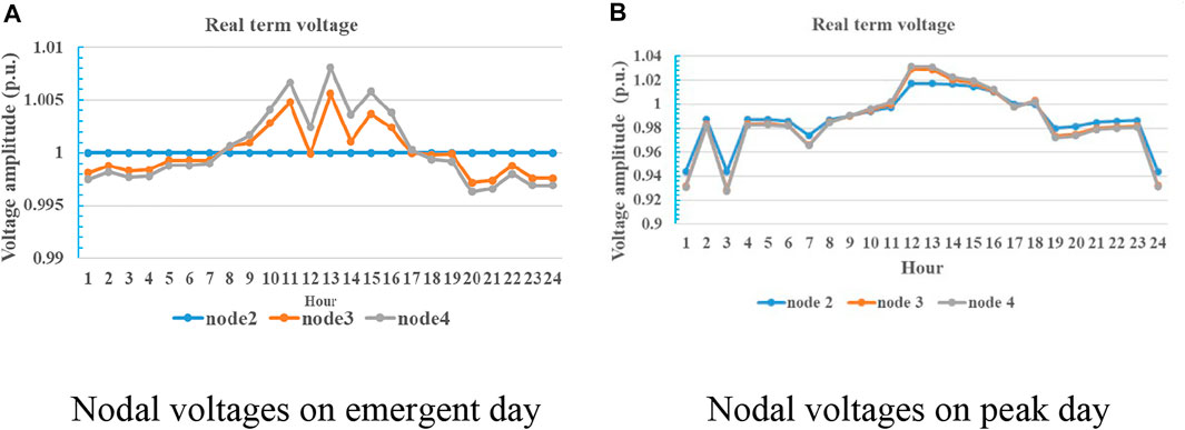
FIGURE 10. Nodal voltages on the emergent day.(A) Nodal voltages on the emergent day and (B) nodal voltages on the peak day.
5.3 Sensitivity analysis
This section elaborates on the sensitivity analysis when different discrete capital costs are considered. As shown in Figure 11, the optimal operation costs vary from 768 to 800 k$, and the total annual CO2 reduction emission costs vary from 1,420 to 1,422 tons with the variation of capital costs. In addition, the total cost saving is at least above 20% and CO2 emission reduction is at least above 25%. Even with the variation of capital costs, the capacity of PV panels remains unchanged as 1,048 kW. However, the total DER capacity of each node varies due to different combinations of technologies. Interestingly, the total capacity of the BESS varies in a very small range, e.g., from 8,102 to 8,119 kWh. The total capacity of DG remains unchanged (420 kW) even with the variation of capital costs because the discrete technology is insensitive to the planning results.

FIGURE 11. Sensitivity analysis with various interest rates. (A) Sensitivity analysis with discrete technology capital cost variations (−10%), (B) sensitivity analysis with discrete technology capital cost variations (−5%), (C) sensitivity analysis with discrete technology capital cost variations (5%), and (D) Sensitivity analysis with discrete technology capital cost variations (10%).
6 Conclusion
This paper investigated the optimal planning and operation of community MGs with the RES and ESS for Lombok Island of Indonesia as a response to the rural electrification program. First, the optimization and constraints for MG planning are presented, which are integrated into the DER-CAM. This study also analyzes the economic benefits and environmental emissions of the optimal sizing and location of the RES and ESS within the MGs. The results of the analyses validate that the DER-CAM can provide the optimal capacities, type, location of various technologies, and optimal energy dispatch for multi-node MGs with optimized total annual costs and total annual CO2 emissions. The planning results demonstrate that the MGs with the RES and ESS contribute to the rural electrification and energy transition of Indonesia, leading to over 100% electrification, 20% cost savings, and 25% CO2 reduction, with interest rates varying from −10% to 10%.
Data availability statement
The original contributions presented in the study are included in the article/Supplementary Material, further inquiries can be directed to the corresponding author.
Author contributions
WK and YG conceived and designed the software simulations. WK and YG performed the simulations. FD, AP, JV, and JM analyzed the data. FD, EK, JV, and JM contributed to the analysis. WK and YG wrote the paper. All authors contributed to the article and approved the submitted version.
Funding
This work was supported by the Tech-IN project (Granted by Danish Ministry for foreign affairs and supported by Danida Fellowship Centre under grant #20-M06-AAU); www.energy.aau.dk/tech-in.
Conflict of interest
The authors declare that the research was conducted in the absence of any commercial or financial relationships that could be construed as a potential conflict of interest.
Publisher’s note
All claims expressed in this article are solely those of the authors and do not necessarily represent those of their affiliated organizations, or those of the publisher, the editors, and the reviewers. Any product that may be evaluated in this article, or claim that may be made by its manufacturer, is not guaranteed or endorsed by the publisher.
References
Bahramara, S., Parsa Moghaddam, M., and Haghifam, M. R. (2016). Optimal planning of hybrid renewable energy systems using HOMER: A review. Renew. Sust. Energ. Rev.62, 609–620. doi:10.1016/j.rser.2016.05.039
Borghei, M., and Ghassemi, M. (2021). Optimal planning of microgrids for resilient distribution networks. Int. J. Electr. Power & Energy Syst.128 (2021), 106682. doi:10.1016/j.ijepes.2020.106682
Cao, X., Wang, J., Wang, J., and Zeng, B. (2019). A risk-averse conic model for networked microgrids planning with reconfiguration and reorganizations. IEEE Trans. Smart Grid11 (1), 696–709. doi:10.1109/tsg.2019.2927833
Cardoso, G., Heleno, M., and DeForest, N. (2019). Remote off-grid microgrid design support tool (ROMDST)-an optimal design support tool for remote, resilient, and reliable microgrids (Phase II, Final Report). Berkeley, CA (United States): Lawrence Berkeley National Lab.
Cardoso, G., Stadler, M., Mashayekh, S., and Hartvigsson, E. (2017). The impact of ancillary services in optimal DER investment decisions. Energy130130, 99–112. doi:10.1016/j.energy.2017.04.124
Chu, S., Cui, Y., and Liu, N. (2017). The path towards sustainable energy. Nat. Mater16, 16–22. doi:10.1038/nmat4834
ESCAP (2020). Energy transition pathways for the 2030 agenda: SDG7 roadmap for Indonesia. Bangkok, Thailand: United Nations Economic and Social Commission for Asia and the Pacific.
Hafez, O., and Bhattacharya, K. (2012). Optimal planning and design of a renewable energy based supply system for microgrids. Renew. Energy45, 7–15. doi:10.1016/j.renene.2012.01.087
Heleno, M., et al. (2017). “Optimal sizing and placement of distributed generation: MILP vs PSO comparison in a real microgrid application,” in Proceedings of the 19th International Conference on Intelligent System Application to Power Systems, San Antonio, TX, USA, September 2017.
Hittinger, E., Wiley, T., Kluza, J., and Whitacre, J. (2015). Evaluating the value of batteries in microgrid electricity systems using an improved Energy Systems Model. Energy Convers. Manag.89, 458–472. doi:10.1016/j.enconman.2014.10.011
Iea, W., and Irena, U. N. S. D. (2021). Tracking SDG 7: The energy progress report 2021. Washington DC: World Bank, 234.
Jung, J., and Villaran, M. (2017). Optimal planning and design of hybrid renewable energy systems for microgrids. Renew. Sustain. Energy Rev.75, 180–191. doi:10.1016/j.rser.2016.10.061
Khare, V., Nema, S., and Baredar, P. (2016). Solar–wind hybrid renewable energy system: A review. Renew. Sustain. Energy Rev.58, 23–33. doi:10.1016/j.rser.2015.12.223
Lee, E. S., Gehbauer, C., Coffey, B. E., McNeil, A., Stadler, M., and Marnay, C. (2015). Integrated control of dynamic facades and distributed energy resources for energy cost minimization in commercial buildings. Sol. Energy122, 1384–1397. doi:10.1016/j.solener.2015.11.003
Madathil Chalil, S., et al. (2017). Resilient off-grid microgrids: Capacity planning and N-1 security. IEEE Trans. Smart Grid96, 6511–6521.
Madathil, S. C., Yamangil, E., Nagarajan, H., Barnes, A., Bent, R., Backhaus, S., et al. (2017). Resilient off-grid microgrids: Capacity planning and N-1 security. IEEE Trans. Smart Grid9 (6), 6511–6521. doi:10.1109/TSG.2017.2715074
Martinez-Frias, J., Aceves, S. M., Ray Smith, J., and Brandt, H. (2008). A coal-fired power plant with zero-atmospheric emissions. J. Eng. gas turbines power130 (2). doi:10.1115/1.2771255
Mashayekh, S., Stadler, M., Cardoso, G., and Heleno, M. (2017). A mixed integer linear programming approach for optimal DER portfolio, sizing, and placement in multi-energy microgrids. Appl. Energy187, 154–168. doi:10.1016/j.apenergy.2016.11.020
Mashayekh, S., Stadler, M., Cardoso, G., Heleno, M., Madathil, S. C., Nagarajan, H., et al. (2018). Security-constrained design of isolated multi-energy microgrids. IEEE Trans. Power Syst.33 (3), 2452–2462. doi:10.1109/TPWRS.2017.2748060
Mendes, G., Ioakimidis, C., and Ferrão, P. (2011). On the planning and analysis of integrated community energy systems: A review and survey of available tools. Renew. Sustain. Energy Rev.15.9, 4836–4854. doi:10.1016/j.rser.2011.07.067
Mizani, S., and Amirnaser, Y. (2009). “Design and operation of a remote microgrid,” in Proceedings of the 2009 35th Annual Conference of IEEE Industrial Electronics, Porto, Portugal, November 2009 (IEEE).
Phase, I. I. (2018). Remote off-grid microgrid design support tool (ROMDST)-An optimal design support tool for remote, resilient, and reliable microgrids.
PLN (2021). Rencana usaha penyediaan tenaga Listrik (RUPTL) PT PLN (persero) 2021-2030. Jakarta: RUPTL.
Prathapaneni, D. R., and Detroja, K. P. (2019). An integrated framework for optimal planning and operation schedule of microgrid under uncertainty. Sustain. Energy, Grids Netw.19, 100232. doi:10.1016/j.segan.2019.100232
Schittekatte, T., Stadler, M., Cardoso, G., Mashayekh, S., and Sankar, N. (2016). The impact of short-term stochastic variability in solar irradiance on optimal microgrid design. IEEE Trans. Smart Grid9 (3), 1647–1656. doi:10.1109/tsg.2016.2596709
Siddaiah, R., and Saini, R. P. (2016). A review on planning, configurations, modeling and optimization techniques of hybrid renewable energy systems for off grid applications. Renew. Sustain. Energy Rev.58, 376–396. doi:10.1016/j.rser.2015.12.281
Stadler, M., Groissbock, M., Cardoso, G., and Marnay, C. (2014). Optimizing distributed energy resources and building retrofits with the strategic DER-CAModel. Appl. Energy132, 557–567. doi:10.1016/j.apenergy.2014.07.041
Stadler, M., Cardoso, G., Mashayekh, S., and Sankar, N. (2016). The impact of short-term stochastic variability in solar irradiance on optimal microgrid design. IEEE Trans. Smart Grid9 (3), 1647–1656.
Stadler, M., Kloess, M., Groissböck, M., Cardoso, G., Sharma, R., Bozchalui, M., et al. (2013). Electric storage in California’s commercial buildings. Appl. Energy104, 711–722. doi:10.1016/j.apenergy.2012.11.033
Wang, J., and Lu, X. (2020). Sustainable and resilient distribution systems with networked microgrids [point of view]. Proc. IEEE108 (2), 238–241. doi:10.1109/jproc.2019.2963605
Wang, Y., Rousis, A. O., and Strbac, G. (2021). A three-level planning model for optimal sizing of networked microgrids considering a trade-off between resilience and cost. IEEE Trans. Power Syst.36 (6), 5657–5669, Nov. doi:10.1109/TPWRS.2021.3076128
Keywords: community microgrid planning, resilience, CO2 reduction, rural electrification, distributed energy resources
Citation: Kang W, Guan Y, Danang Wijaya F, Kondorura Bawan E, Priyo Perdana A, Vasquez JC and M. Guerrero J (2023) Community microgrid planning in Lombok Island: an Indonesian case study. Front. Energy Res. 11:1209875. doi: 10.3389/fenrg.2023.1209875
Received: 21 April 2023; Accepted: 26 June 2023;
Published: 17 July 2023.
Edited by:
Mingfei Ban, Northeast Forestry University, ChinaReviewed by:
Shuan Dong, National Renewable Energy Laboratory (DOE), United StatesJiyu Wang, National Renewable Energy Laboratory (DOE), United States
Copyright © 2023 Kang, Guan, Danang Wijaya, Kondorura Bawan, Priyo Perdana, Vasquez and M. Guerrero. This is an open-access article distributed under the terms of the Creative Commons Attribution License (CC BY). The use, distribution or reproduction in other forums is permitted, provided the original author(s) and the copyright owner(s) are credited and that the original publication in this journal is cited, in accordance with accepted academic practice. No use, distribution or reproduction is permitted which does not comply with these terms.
*Correspondence: Yajuan Guan, eWd1QGVuZXJneS5hYXUuZGs=