Ultra-short-term power load forecasting method based on stochastic configuration networks and empirical mode decomposition

Ultra-short-term power load forecasting (USTPLF) can provide strong support and guarantee the decisions on unit start-up, shutdown, and power adjustment. The ultra-short-term power load (USTPL) has strong non-smoothness and nonlinearity, and the time-series characteristics of the load data themselves are difficult to explore. Therefore, to fully exploit the intrinsic features of the USTPL, a stochastic configuration networks (SCNs) USTPLF method based on K-means clustering (K-means) and empirical mode decomposition (EMD) is proposed. First, the load data are decomposed into several intrinsic mode functions (i.e., IMFs) and residuals (i.e., Res) by EMD. Second, the IMFs are classified by K-means, and the IMF components of the same class are summed. Third, the SCNs is used to forecast the electric load on the basis of the classified data. Lastly, on the basis of the real load of Shenzhen City, the proposed method is applied for emulation authentication. The result verifies the efficiency of the proposed measure.

1 Introduction

1.1 Literature review

Ultra-short-term power load forecasting (USTPLF) is an essential reference for real-time dispatching orders and a fundamental basis for determining real-time tariffs, grid peaking, and valley filling (Lin et al., 2022; Lin et al., 2022). In recent years, the increase in distributed energy sources and the grid connection of new energy generation has led to the strong nonlinearity, non-smoothness, and randomness of ultra-short-term power load (USTPL), which brings challenges to USTPLF. Accurate USTPLF can realize the advanced control of automatic generation, reduce the adjustment pressure on automatic generation control, guarantee the stable operation of the power system, and enhance the efficiency of grid dispatch (Yan et al., 2021; Pham et al., 2022; Sun and Cai, 2022).

Research on power load forecasting methods. USTPLF is mainly divided into traditional statistical methods and machine learning methods. The traditional statistical methods mainly include the linear regression model (Liang and Tang, 2022), the Kalman filter method (Guo et al., 2022), and the time series model (He et al., 2022). Literature (Kim et al., 2022) used the curve extrapolation method for USTPLF based on short-term load forecasting results, eliminating the influence of holidays and load inflection points on the forecasting results. Literature (Guan et al., 2013) used the Kalman filter to generate prediction intervals and perform USTPLF automatically. Traditional statistical methods have high data requirements and cannot obtain accurately predicted load values when dealing with large amounts of nonlinear load data. Machine learning methods mainly include BP neural networks (Chen et al., 2023; da Silva and de Andrade, 2016), support vector machines (SVM) (Jiang et al., 2020), and deep learning (Tan et al., 2020). In Literature (Huang et al., 2022), a two-way weighted LS-SVM was used for USTPLF, which proved the characteristic of “large near and small far” for USTPLF. It did not rely on long-range data and considered near-term load data more. However, the fast leave-one-out method could not find the optimal parameters of the LS-SVM, which affected the prediction accuracy. Literature (Madhukumar et al., 2022) first used phase space reconstruction to find the intrinsic pattern between load data, established an SVM load prediction model after determining the import and output data, and optimized the SVM parameters by using an improved particle swarm algorithm to enhance the model prediction capability. Literature (Mir et al., 2021) adopted an enhanced firework algorithm to find the optimal weights and thresholds of the extreme learning machine to overcome the problem of model instability caused by randomly generated weights and thresholds of the extreme learning machine in USTPLF. Literature (Gunawan and Huang, 2021) used a stochastic distributed embedding framework and a BP neural network to solve the problem of low accuracy of USTPLF caused by a small amount of data. However, the BP is prone to overfitting when the import data are significant. In Literature (Xuan et al., 2021), the tree model in the lightweight gradient boosting machine (Light-BM) was used to evaluate the importance of each import feature quantitatively. At the same time, an attention mechanism was introduced to give different weights to different time series information, which overcomes the problem of easy loss of crucial information in gated recurrent neural networks when the import time series is longer. Additionally, in the field of wind power forecasting, several studies have proposed novel models to enhance the accuracy of wind power prediction. For instance, the study by (Shahid et al., 2021) presented a novel genetic LSTM model for wind power forecast, which leverages the genetic algorithm to optimize the LSTM network parameters and improve the forecasting accuracy. Furthermore, in financial market forecasting, the study conducted by (Bukhari et al., 2020) proposed a Fractional Neuro-Sequential ARFIMA-LSTM model, which integrates the ARFIMA model with LSTM to forecast financial market dynamics more accurately In Literature (Ageng et al., 2022), a method of USTPLF based on an extreme gradient enhancement algorithm (XGBOOST) combined with a long- and short-term memory neural network (LSTM) was proposed to enhance the accuracy of USTPLF by using XGBOOST for point prediction and then using LSTM for probabilistic prediction. The machine learning method is good at handling a large amount of nonlinear data. It has a good generalization ability to anonymous data, but it often affects the USTPLF accuracy due to improper human-set parameters.

A study on the Import feature of USTPLF. USTPLF is usually influenced by the load data in the hours before the moment to be predicted and external factors, e.g., wind force and wind direction do not change much during this period; hence, the external factors, such as wind force and wind direction, are not considered in USTPLF (Bouktif S et al., 2018). Tapping the laws of the electric load data themselves is the key to improving the accuracy of USTPLF. Literature (Zhao et al., 2019) used the attention mechanism to assign different weights to the import data so that the gated recurrent unit (GRU) focuses on learning important information, which overcomes the disadvantage that the GRU tends to lose sequence information in the learning process and improves the prediction efficiency. However, the attention mechanism only exploits the shallow features of the load data and does not perform deep mining of the data themselves. Literature (Li et al., 2017) utilized wavelet decomposition to decompose the load and a second-order gray neural network to predict and sum the components. Another study by (Shahid et al., 2020) introduced a novel Wave nets long short-term memory paradigm for wind power prediction, which combines the Wave nets model with LSTM to capture the long-term dependencies in wind power time series data. Literature (Kong et al., 2020) used multiple clustering analysis to filter the import features, wavelet decomposition to classify the load into high- and low-frequency components, a convolutional neural network (CNN) to predict the high-frequency components, and a multiplexed CNN (MCNN) to predict low-frequency components. Cluster analysis and wavelet decomposition can fully exploit the inherent features and patterns of load data and enhance the accuracy of USTPLF. Although the wavelet decomposition method can decompose load sequences, the selection of wavelet basis functions and decomposition layers has a significant impact on the decomposition effect for sequences with poor stability, which increases the prediction difficulty. Literature (Tang et al., 2019) decomposed the load sequence into different modal components via empirical mode decomposition (EMD) and predicted the modal components through deep belief networks and bi-directional recurrent neural networks. In Literature (Li et al., 2020), the EMD with adaptive noise was used to decompose the load sequence into different components, and the SVM with optimized parameters using the whale algorithm was employed to predict the different components with enhanced prediction accuracy. The EMD method is adaptive and can decompose the load on the basis of its time-series characteristics without artificially setting parameters, simplifying the prediction difficulty. Therefore, the decomposition of the prediction model’s import load data can explore the data’s laws. However, it also increases the prediction time and reduces the prediction efficiency because of the excessive decomposed components. A brief summary of the studied literature is presented in Table 1. In the research of power load forecasting, machine learning methods such as neural networks, support vector machines, and deep learning have shown excellent performance in handling large amounts of nonlinear data. Researchers have employed techniques such as attention mechanisms, wavelet decomposition, and clustering analysis to uncover the intrinsic patterns and features of load data, aiming to improve prediction accuracy. However, the decomposition methods may increase prediction time and reduce efficiency. Therefore, when selecting a forecasting method, it is necessary to consider the characteristics of load data and the requirements for prediction accuracy.

TABLE 1

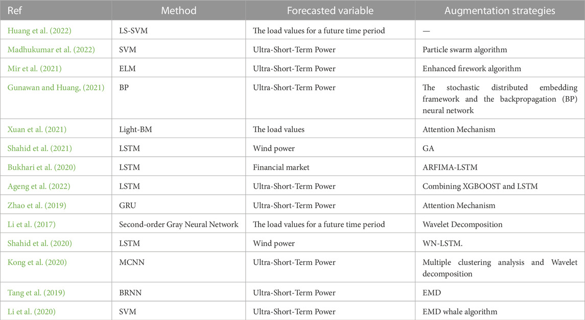
TABLE 1. Literature review summary.

1.2 Motivation

Despite the widespread application of data-driven methods in feature construction and model training, they are not without limitations. One notable drawback is their excessive reliance on parameter optimization algorithms, such as particle swarm optimization or the whale optimization algorithm, which necessitates parameter tuning and manual intervention. This reliance adds complexity and subjectivity to the methods. Another significant limitation is the substantial impact of parameter selection on the results. In certain methods, such as selecting wavelet basis functions and determining decomposition levels, the choice of parameters heavily influences the prediction outcomes. Determining the appropriate parameters often requires expertise and rigorous experimental investigation, further complicating the methods and introducing uncertainty. Additionally, the need for different parameter settings across diverse datasets and problems can impede the methods’ generalizability.

These limitations pose challenges and constraints in the practical application of data-driven methods. To overcome these issues, a novel approach that integrates Empirical Mode Decomposition (EMD), K-means clustering, and stochastic configuration networks (SCNs) has been proposed. This approach offers a unique and innovative solution that effectively addresses the aforementioned limitations, thereby enhancing the accuracy and robustness of load forecasting. Finally, the ultra short term power load (USTPL) has strong non smoothness and nonlinearity, making it difficult to explore the time series characteristics of the load data itself.

1.3 Contributions

This approach makes the following contributions:

(1) It introduces a combined method based on Empirical Mode Decomposition (EMD), K-means clustering, and stochastic configuration networks (SCNs) for ultra-short-term load forecasting. By decomposing the load data into Intrinsic Mode Functions (IMFs) and residuals using EMD, and then classifying the IMFs with K-means clustering, the method effectively explores the intrinsic features of the load data.

(2) The utilization of stochastic configuration networks as the training model is a significant contribution. SCNs possess adaptive characteristics and require minimal manual parameter settings. They are capable of leveraging the key information in the load sequence and achieving accurate predictions.

(3) By using the classified components as input features for training SCNs, the method reduces the dependence on parameters, thus enhancing the reliability and efficiency of ultra-short-term load forecasting.

In summary, the proposed approach based on EMD, K-means, and SCNs effectively tackles the limitations of data-driven methods while enhancing the accuracy and robustness of load forecasting. By effectively extracting the intrinsic features of historical load data and reducing dependence on parameters, this approach offers a more efficient and accurate solution for ultra-short-term load forecasting, surpassing the performance of LSTM and SVM models.

The study is organized as follows: Section 2 provides the background and objectives of the research, highlighting the existing challenges in the field and clarifying the research purpose and questions. Section 3 introduces the methodology or strategy employed to address the research problem. Section 4 presents the approach used for feature extraction from the load data. Section 5 describes the application of the K-means clustering algorithm to group the load sequences. Section 6 outlines the load forecasting model based on stochastic configuration networks. Section 7 provides a description of the dataset used in the study.

2 Problem description

The difference between the USTPLF and the short-term power load forecast is that it follows the principle of large near and small far, i.e., the first n hours of the time to be forecasted are crucial for the USTPLF. Short-term power load forecasting is to forecast a load of a day on the day to be forecasted simultaneously. It cannot take into account the interactions between the loads at each moment on the day to be forecasted, whereas USTPLF is hourly granular. The accuracy rate is higher, and the moment to be forecasted is very close to the first n hours. External influencing factors, such as wind force, wind direction, and humidity, do not change much. Therefore, in USTPLF, external influences on the load are usually not considered. The key to improving the accuracy of USTPLF is digging deeper into the laws in the load data themselves. Traditional forecasting methods have limited ability to map nonlinear data, and the LSTM has excessive artificially set parameters, which is prone to the problem of time series information loss and affects its forecasting accuracy. SCNs are suitable for USTPLF given the advantages of less artificially set parameters, high intelligence, and shorter time required for forecasting. The application of our research lies in Ultra-Short-Term Power Load Forecasting (USTPLF). USTPLF aims to accurately predict power load variations in the near future. This application is crucial for the operation and scheduling of power systems, enabling power companies to plan generation capacity, optimize grid operations, and enhance energy utilization efficiency. The problem description of USTPLF is shown in Figure 1.

FIGURE 1

FIGURE 1. Description of the USTPLF problem.

3 Strategy structure

Suppose only the extrinsic features of load data are observed without digging deeper into the intrinsic features of the load data themselves. In this case, the prediction accuracy will decrease, and the prediction time will increase. EMD can decompose the original load data into several load sequence components to explore the original load data’s intrinsic features deeply. K-means can integrate the components to reduce the prediction time. Therefore, this study proposes an SCNs ultra-short-term load forecasting method based on K-means and EMD. First, missing load data are filled. Second, EMD is used to decompose the load data into several IMFs and residuals to reduce the randomness and volatility of the load data. Third, K-means is used to classify several components, and the components contained at the center of each cluster are summed. Lastly, the summed components are imported to stochastic configuration networks for training. The mean absolute error (MAE), mean absolute percentage error (MAPE), and root-mean-square error (RMSE) are chosen to measure the performance of the prediction method. The specific implementation strategy of the method is shown in Figure 2.

FIGURE 2

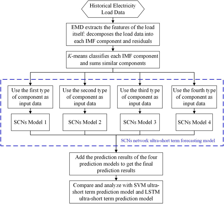
FIGURE 2. Strategy diagram of the USTPLF method.

4 Load data feature extraction

USTPLF predicts the load changes in the next few hours. During this period, the weather, temperature, humidity, and other external factors have minimal changes, so the influence of external factors on the load is not considered. When forecasting, only observing the external characteristics of the load data and not digging into the internal laws of the load data themselves will reduce the forecasting accuracy. Therefore, determining how to mine the inherent characteristics of load data is important. The load series is decomposed into IMFs and residuals by EMD (Gloersen and Huang, 2003) in accordance with the time scale of the load data themselves. Each IMFs represents the characteristic components of the load series on this time scale. The characteristic law of each IMF is the characteristic law of the load data themselves. The composition of the IMF must meet two characteristics: ① The difference between the number of extreme points and the number of zero points of the intrinsic mode component cannot be greater than 1. ② The average value of the upper and lower envelopes of the eigenmode components at any time is zero (Yang et al., 2018).

Algorithm 1 is a method used for Empirical Mode Decomposition (EMD) of historical power load data. The algorithm takes historical power load data and a preset value R as input, and it outputs the power load sequence components and the residual error of the power load series, R(t). The algorithm begins by extracting all maximum points (e max(t)) and minimum points (e min(t)) from the load data (P(t)). It then calculates the average of the load data and generates a new load series based on this average. Next, the algorithm checks if the difference between the number of extreme points and the number of zero points is not greater than 1 and if specific conditions are met. If these conditions are satisfied, the algorithm selects the first Intrinsic Mode Function (IMF), which represents a characteristic component of the load series on a particular time scale. It also calculates the residual of the load series. The algorithm further evaluates if the residual is less than the preset value R and if it represents a monotonic load sequence. If both conditions are met, the algorithm retains the residual as part of the decomposition process. Otherwise, it returns to step 1 and repeats the process with the historical power load data. The specific steps of EMD decomposition of power load data are shown in Figure 3; Algorithm 1.

FIGURE 3

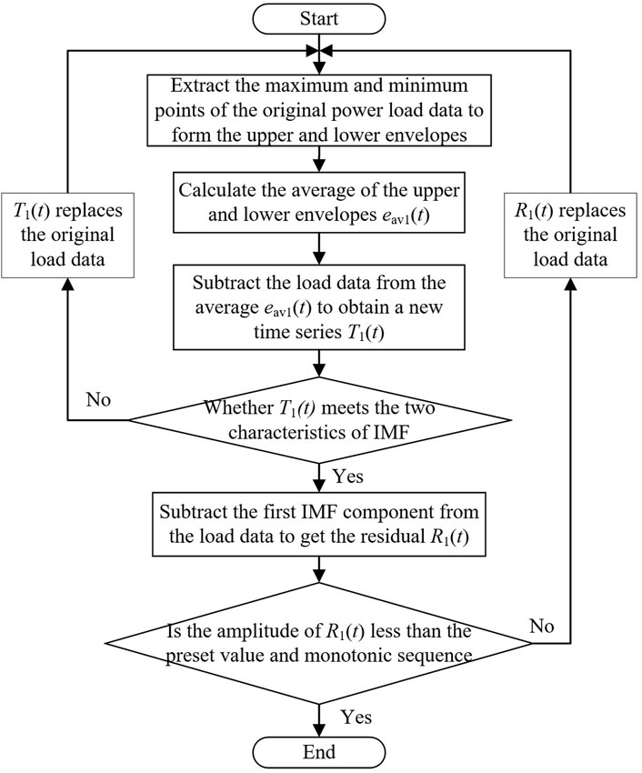
FIGURE 3. Flowchart of EMD breakdown load data.

Algorithm 1. EMD decomposes historical power load data

Input: Historical power load data $P\left(t\right),t=\mathrm{1,2},\cdots ,4032$; Preset value R

Output: Power load sequence component $f_{\mathrm{I}\mathrm{M}\mathrm{F}k}\left(t\right),k=\mathrm{1,2},\cdots ,9$, Residual error of power load series R(t)

1:  Extract all maximum points e_max(t) and minimum points e_min(t) in load data P(t)

2:  Calculate the average: $e_{av1}\left(t\right)=\frac{e_{\max }\left(t\right)+e_{\min }\left(t\right)}{2}$

3:  Calculate new load series $T_1\left(t\right)=P\left(t\right)-e_{av1}\left(t\right)$;

4:  If the difference between the number of extreme points of $T_1\left(t\right)$ and the number of zero points is not greater than 1 and $e_{av}\left(t\right)=0$

5:   The first IMF $f_{\mathrm{I}\mathrm{M}\mathrm{F}1}\left(t\right):=T_1\left(t\right)$

6:   Calculate the residual of load series $R_1\left(t\right)=P\left(t\right)-f_{\mathrm{I}\mathrm{M}\mathrm{F}1}\left(t\right)$

7:    If$R_1\left(t\right)$ is less than the preset value R and is a monotonic load sequence

8:     The residual $R\left(t\right):=R_1\left(t\right)$

9:    Else

10:     The historical power load data $P\left(t\right):=R_1\left(t\right)$ go to step 1

11:    End if

12:  Else

13:   The historical power load data $P\left(t\right):=T_1\left(t\right)$ go to step 1

14:  End if

5 K-means of load series

After load feature extraction, the load data are decomposed into several IMFs and residuals. If all the IMFs and residuals are imported into the SCNs as import data for training, it will lead to a large amount of data and increase the prediction time. Given its real-time characteristics (Ding et al., 2020), USTPLF requires high forecasting speed. K-means is used to integrate IMFs and residuals to reduce the import data of the SCNs and enhance the forecasting speed. First, K-means centers are built, and the coordinates of the clustering centers are determined. Then, the Euclidean distances of each IMF, each residual, and the cluster center are calculated. The calculation formula is shown in Formula (1), and each IMF and each residual are classified in accordance with the Euclidean distance. Lastly, the IMFs of the same category are added, and the added components are used as the import data of the SCNs ultra-short-term load forecasting model. The process is shown in Figure 4.

$d_j=\sqrt{{\displaystyle \sum _{s=1}^n}{\left(x_s-p_{fs}\right)}^2}(1)$

where $x_s\left(s=\mathrm{1,2},\cdots ,n\right)$ is the load value of the IMF component, and $p_{fs}\left(f=1,2,\cdots ,z;s=1,2,\cdots ,n\right)$ is the coordinate value of the fth cluster center.

FIGURE 4

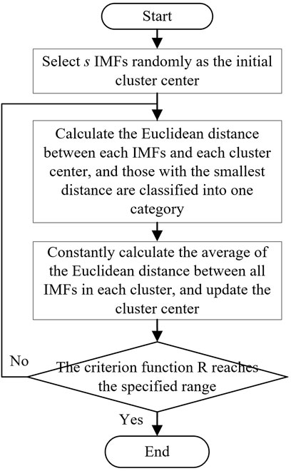
FIGURE 4. Flowchart of K-means cluster with IMFs.

6 Load forecasting model based on stochastic configuration networks

SCNs have the advantages of fewer parameters set manually, automatically adjusting the weight of each unit in accordance with the prediction error, avoiding the problem of affecting the accuracy of load forecasting caused by improper parameter selection, and rapid selection of hidden parameters through its evaluation function, thus improving the forecasting efficiency. Therefore, SCNs are used to forecast USTPLs with high accuracy and speed requirements. SCNs are random-weighted neural networks with a supervision mechanism proposed by Wang and Li, (2017). Their structure includes an input layer, a variable hidden layer, and an output layer. Unlike the traditional feedforward neural network, SCNs can start from a small network with minimal human intervention, randomly select import weights and thresholds, gradually increase the number of hidden layer neuron nodes, and use the least squares method to calculate the output weights and thresholds until the training accuracy of the network meets the termination conditions. In addition, SCNs add an evaluation function for random parameters and adaptively select the range of random parameters.

Suppose we build an SCNs model with L-1 hidden layer nodes, and its basic mapping relationship is

$f_{L-1}\left(X\right)={\beta }^{T}H={\displaystyle \sum _{j=1}^{L-1}}{\beta }_j{g}_j\left(w_j^{T}X+b_j\right)\left(L=\mathrm{1,2},\dots ,m;f_0=0\right)(2)$

where ${\beta }_j$ is the output weight matrix of the jth hidden layer node; $X=\left\{X_1,X_2,\dots ,X_N\right\}$ is the import characteristic matrix, e.g., $X_1={\left[x_1,x_2,\cdots x_M\right]}^T$; $w_j$ and $b_j$ are the import weight and threshold matrix of the jth hidden layer node, respectively; $g_j$ is the sigmoid activation function.

$g_j=g\left(w_j^{T}X+b_j\right)=\frac{1}{1+\exp \left(-w_j^{T}X+b_j\right)}(3)$

When the model is calculated for the first time, the difference between the model output and the real value is defined as

$e_{L-1}=f-f_{L-1}=\left[e_{L-\mathrm{1,1}},e_{L-\mathrm{1,2}},\dots ,e_{L-1,m}\right](4)$

where $e_{L-1}$ represents the difference between the number of different nodes, and $e_{L-1,K}$ is the difference of corresponding characteristics of different nodes.

When the error does not meet the set value, $g_L$ and b_g are randomly generated in accordance with Formula (5)–Formula (7), and the updated output weight value ${\beta }_L$ is calculated. A hidden layer node is added, and the model output is updated to $f_L\left(X\right)=f_{L-1}\left(X\right)+{\beta }_L{g}_L$ to achieve the purpose of correcting the residual. As a result, the output predicted value is closer to the real value, and the update process is until the error meets the set value. The update function is

$〈e_{L-1,q},g_L^2〉\ge b_g^2{\delta }_{L,q},q=\mathrm{1,2},\cdots m(5)$

${\beta }_{L,q}=\frac{〈e_{L-1,q},g_L〉}{{‖g_L‖}^2},q=\mathrm{1,2},\dots ,m(6)$

$\left\{\begin{array}{l}{\delta }_L={\displaystyle \sum _{q=1}^m}{\delta }_{L,q}\\ {\delta }_{L,q}=\left(1-r-{\mu }_L\right){‖e_{L-1,q}‖}^2\end{array}\right.(7)$

The evaluation function is defined as follows:

${\xi }_{L,q}=\frac{{\left(e_{L-1,q}{\left(X\right)}^T•g_L\left(X\right)\right)}^2}{g_L{\left(X\right)}^T•g_L\left(X\right)}-\left(1-r-{\mu }_L\right)e_{L-1,q}{\left(X\right)}^T•e_{L-1,q}\left(X\right)(8)$

where $g_L\left(X\right)=g_L\left(w_L^{T}X+b_L\right)$; 0 < r < 1; ${\mu }_L$ is a sequence of non-negative real numbers. The larger the value of the evaluation function ${\xi }_{L,q}$, the better the model parameter configuration, and the faster the convergence of the stochastic configuration networks.

The construction of the SCNs ultra-short-term load forecasting model is shown in Figure 5. The model comprises 144 neurons in the input layer, 261 neurons in the hidden layer, and 48 neurons in the output layer. The algorithm starts with initialization and enters a while loop. In each iteration, it performs nested loops to randomly assign weights and calculate the evaluation function and error. If the evaluation function meets certain criteria, the weights are stored. If the stored set is not empty, the algorithm finds the weights that maximize the evaluation function and generates a matrix. Otherwise, it randomly fetches weights and continues the process. After the iterations, the algorithm calculates the optimal output weight and output error. It then updates the weights and continues the loop until the specified conditions are met. Finally, the algorithm returns the predicted value of load series components in the time period to be predicted. The detailed steps of the SCNs ultra-short-term load forecasting model are given in Algorithm 2.

FIGURE 5

FIGURE 5. SCNs ultra-short-term load forecasting model.

Algorithm 2. SCNs

Input: Power load sequence component $X=\left\{X_1,X_2,\dots ,X_N\right\},N=21$; Expected output corresponding to the power load sequence component $T=\left\{t_1,t_2,\dots ,t_N\right\}$; Number of neurons in the maximum hidden layer of SCNs $L_{\max }$; Error tolerance $\epsilon$; Maximum number of random configurations $T_{\max }$; Value range of random weight $\mathrm{\Upsilon }=\left\{{\lambda }_{\min },\dots ,{\lambda }_{\max }\right\}$;

Output: Predicted value of load series components in the time period to be predicted $P=\left(P_1,P_2,\cdots ,P_m\right),m=48$

1:  Initialization:$e_0={\left[t_1,t_2,\dots ,t_N\right]}^T$,$0<r<1$,$\mathrm{\Omega },W=\varphi$;

2:  while$L\le L_{\max }$ and ${‖e_0‖}_F>\epsilon$, do

3:   for$\lambda \in \mathrm{\Upsilon }$, do

4:    for$k=\mathrm{1,2},\dots ,T_{\max }$, do

5:     Randomly assign $w_L$ and $b_L$ from intervals ${\left[-\lambda ,\lambda \right]}^M$ and $\left[-\lambda ,\lambda \right]$, respectively;

6:    Calculate $g_L\left(X\right)=$$\left[g_L\left(w_L^T{x}_1+b_L\right),g_L\left(w_L^T{x}_2+b_L\right),\dots ,g_L\left(w_L^T{x}_N+b_L\right)\right]$;

7:    Calculate the evaluation function ${\xi }_{L,K}$;

8:    Calculate${\mu }_L=\left(1-r\right)/\left(L+1\right)$;

9:     if$\min \left\{{\xi }_{L,1},{\xi }_{L,2},\dots ,{\xi }_{L,K}\right\}\ge 0$then

10:      Store $w_L$ and $b_L$ in $W$ and ${\xi }_L={\displaystyle \sum _{k=1}^K}{\xi }_{L,k}$ in $\mathrm{\Omega }$;

11:     else

12:      go to step 7

13:     end if

14:    end for

15:    if$W$ is not an empty set then

16:     Find the $w_L^{*}$ and $b_L^{*}$ that make ${\xi }_L$ the largest in $\mathrm{\Omega }$, and then generate the matrix $\left[g_1^{*},g_2^{*},\dots ,g_L^{*}\right]$

17:     Break (go to step 24)

18:    else

19:     Randomly fetch $\tau \in \left(\mathrm{0,1}-r\right)$, update $r$: $r=r+\tau$, go back to step 7

20:    end if

21:   end for

22:           Calculate the optimal output weight$\left[{\beta }_1^{*},{\beta }_2^{*},\dots ,{\beta }_L^{*}\right]=\underset{\beta }{\mathrm{argmin}}‖f-{\displaystyle \sum _{j=1}^L}{\beta }_j{g}_j\left(w_j^{T}X+b_j\right)‖$

23:   Calculate output error$e_L=e_{L-1}-{\beta }_L^{*T}{g}_L^{*}$;

24:   To update$e_0$: $e_0=e_{L-1}$; $L$: $L=L+1$;

25:  end while

26:  Return${\beta }_1^{*},{\beta }_2^{*},\dots ,{\beta }_L^{*}$; $w^{*}=\left[w_1^{*},w_2^{*},\dots ,w_L^{*}\right]$; $b^{*}=\left[b_1^{*},b_2^{*},\dots ,b_L^{*}\right]$

7 Example analysis

7.1 Dataset description

This study adopts Shenzhen’s power load data set from June 2 to 13 July 2017, with a total of 42 days of load data. The sampling interval of load data is 15 min, with a total of 4,032 data points. The time period to be predicted is 12:00–24:00 on July 13.

The power load data set is checked. If there is a missing value, it is filled with the average value. The data in this dataset are complete, and whether to fill in missing values is optional.

7.2 Performance evaluation index

MAE, MAPE, and RMSE are used as evaluation indicators of prediction methods. The calculation formulas are as follows:

$\mathrm{M}\mathrm{A}\mathrm{E}=\frac{1}{N}{\displaystyle \sum _{i=1}^N}\left|y_i^{\prime }-y_i\right|(9)$

$\mathrm{M}\mathrm{A}\mathrm{P}\mathrm{E}=\frac{1}{N}{\displaystyle \sum _{i=1}^N}\left|\frac{y_i^{\prime }-y_i}{y_i}\right|\times 100(10)$

$\mathrm{R}\mathrm{M}\mathrm{S}\mathrm{E}=\sqrt{\frac{1}{N}{\displaystyle \sum _{i=1}^N}{\left(y_i^{\prime }-y_i\right)}^2}(11)$

where $y_i^{\prime }$ is the predicted load value, and $y_i$ is the actual load value.

7.3 Historical load data decomposition

The EMD method is used to decompose the historical power load data, and a total of 10 components are obtained, including 9 IMFs and 1 residual, which are recorded as e1–e10. The decomposed load series is shown in Figure 6. The frequency of each IMF component is relatively stable and shows evident periodicity. Through its periodicity, the characteristics of the load series can be mined.

FIGURE 6

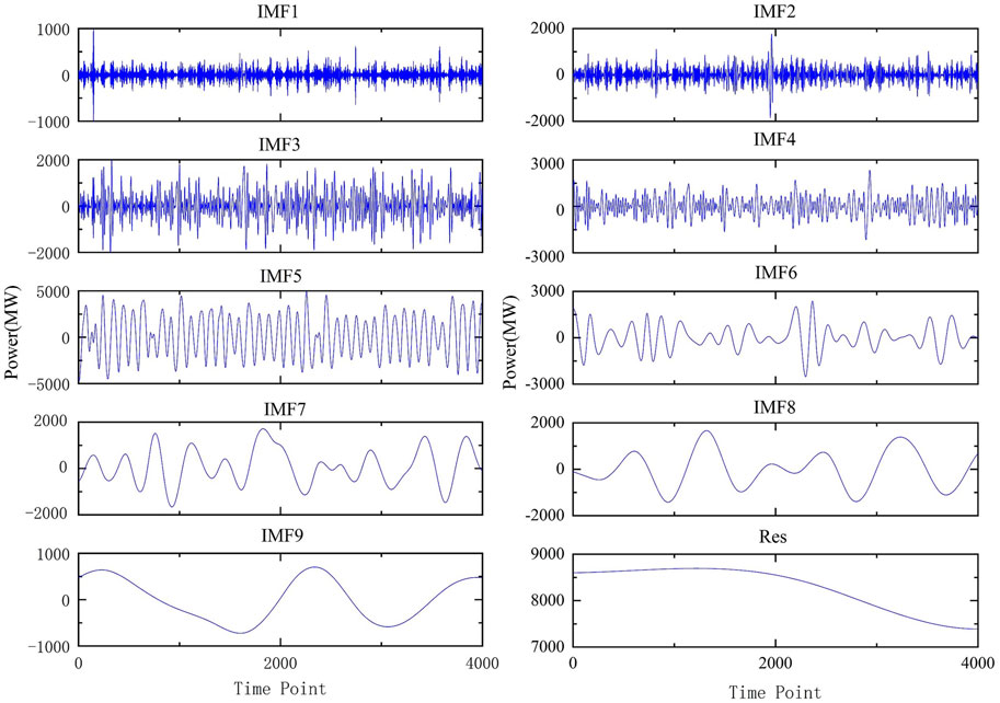
FIGURE 6. IMFs and Res after load data decomposition.

From Figure 6, the EMD decomposes the historical power load data into 10 components. If these 10 components are imported into the SCNs as import data for training, the calculation amount and prediction time of the model will increase. Therefore, to enhance the prediction speed, K-means is used to integrate all components, which are then used as import data for prediction. The center point is set to 4, and the effect of clustering each IMF component and Res is shown in Figure 7. Each component is divided into four categories. The components in the same category are added to obtain the new load series components d1–d4. The new components d1–d4 are predicted as the import data of the stochastic configuration networks model, and the sum of the four prediction results is the USTPLF result.

FIGURE 7

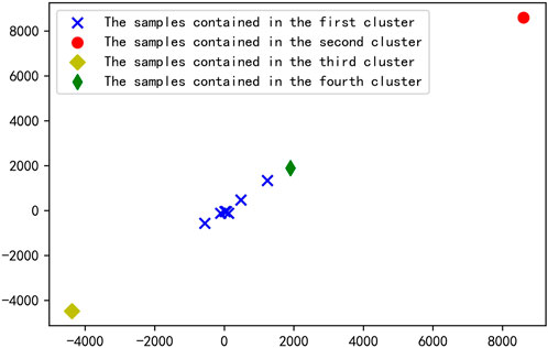
FIGURE 7. Effect of the clustering of each component.

7.4 Parameter settings of stochastic configuration networks

Before USTPLF, the SCNs should be trained. The evaluation index used in training is the RMSE of the load forecast value and the actual value. The relationship between the training error of SCNs and the number of hidden layer nodes is shown in Supplementary Appendix SA1 and Figure 8.

FIGURE 8

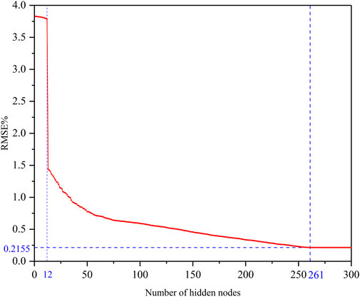
FIGURE 8. Training error value corresponding to the number of hidden layer nodes.

From the figure, when the number of hidden layer nodes is small, the training error of SCNs is significant and does not change as the number of nodes increases. When the number of hidden layer nodes increases to 13, the training error of SCNs decreases significantly, continues to decrease as the number of nodes increases, and finally tends to stabilize. At this time, the training RMSE of SCNs is 0.2155%.

The specific parameter settings of SCNs are as follows: number of neurons in the maximum hidden layer $L_{\max }=300$, error tolerance $\epsilon =0.001$, random weight range $\mathrm{\Upsilon }$ = [ 0.1,0.15,0.2, … ,8], and maximum number of random configurations $T_{\max }=50$.

7.5 Load forecasting and analysis

This study sets every 3 days as a sample, having a total of 39 groups of samples. Of them, 80% are taken as the training set, with a total of 32 groups of samples; 20% are taken as the test set, with a total of 7 groups of samples. The import data of each group of samples are the load data of the first and second days of the sample and the load data of the third day from 00:00 to 11:45, a total of 144 data; the output data are the load data of the third day from 12:00 to 23:45, a total of 48 data. The first load series component d1, the second load series component d2, the third load series component d3, and the fourth load series component d4 are imported into the SCNs for training. The predicted values are compared. The actual load values in the 12:00–24:00 time period of each load series component to be predicted are shown in Figure 9. The predicted values of the four components are added to determine the load values of the period from 12:00 to 24:00 on the day. The comparison with the actual value is shown in Figure 10.

FIGURE 9

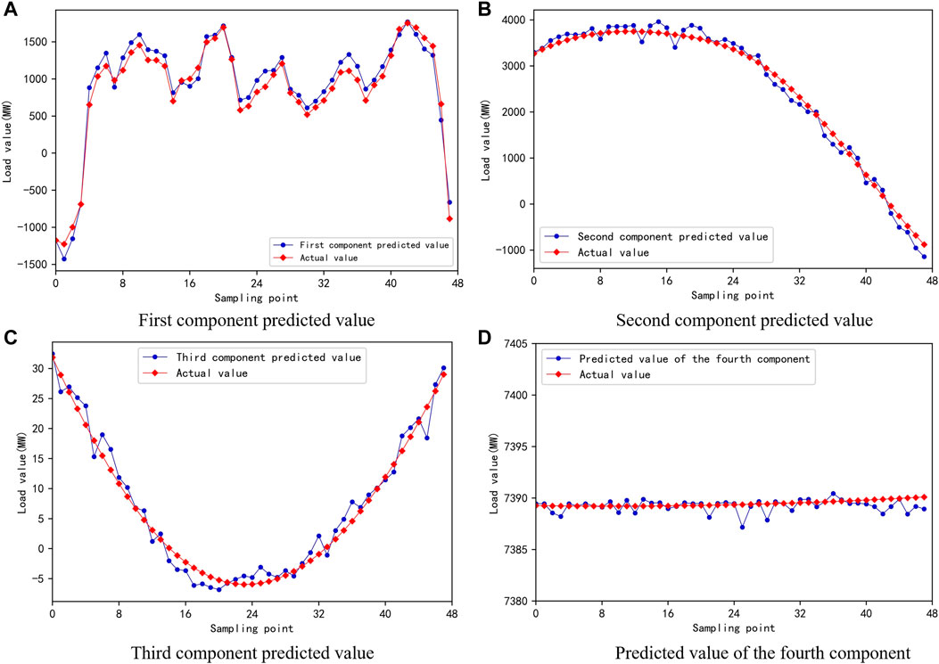
FIGURE 9. Comparison between predicted and actual values of four components. (A) First component predicted value. (B) Second component predicted value. (C) Third component predicted value. (D) Predicted value of the fourth component.

FIGURE 10

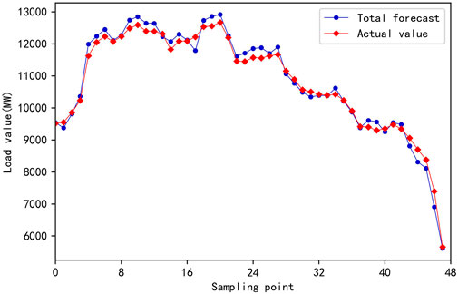
FIGURE 10. Comparison between total predicted value and actual value.

The four methods are programmed separately, and the numerical examples are analyzed.

(1) Method 1: The historical power load data without EMD and K-means processing are taken as the import data to build the SCNs model, which is called SCNs.

(2) Method 2: The four load series components obtained after EMD and K-means processing are taken as import data, four SVM models are constructed, the prediction results are summed, and the method is called EKSVM.

(3) Method 3: The four load series components obtained after EMD and K-means processing are taken as import information, four LSTM models are set, the prediction results are summed, and the method is called EKLSTM.

(4) The proposed measure in this thesis is to construct four SCNs models and sum the prediction results by using the four load series components obtained after EMD and K-means processing as import data. The method is named EKSCNs.

The MAE, MAPE, and RMSE of the four measures are shown in Table 2. The error between the predicted value and the real value at 48 time points in the time period from 12:00 to 24:00 on 12 July 2017 is shown in Figure 11. Figure 12 presents a comparison between the predicted loads of the four methods and the real loads at 48 time points. The scatter plots between the predicted values of the four methods and the actual values are given in Figure 13. The smaller the difference between the predicted and actual values, the closer the point in the figure is to the diagonal line.

TABLE 2

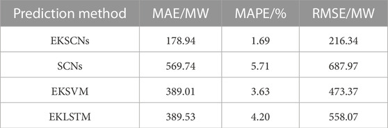
TABLE 2. MAE, MAPE, and RMSE of the four methods.

FIGURE 11

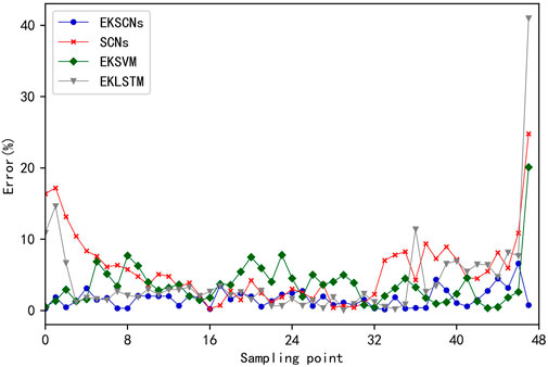
FIGURE 11. Comparison of errors of the four measures.

FIGURE 12

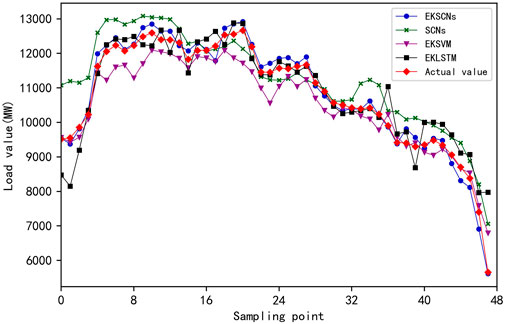
FIGURE 12. Comparison between the predicted values of the four methods and the real values.

FIGURE 13

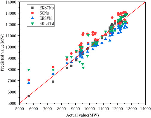
FIGURE 13. Scatter chart of the predicted values of the four methods and the actual values.

From Figures 11–13; Table 2, when SCNs are also used, the load series components obtained after EMD and K-means processing and used as import data show reductions of 390.8 MW, 4.02%, and 471.63 MW in MAE, MAPE, and RMSE, respectively, compared with the historical load data that are not preprocessed. This result verifies the effectiveness of using EMD and K-means in preprocessing historical load data. In the same case of EMD and K-means processing, EKSCNs is the closest to the slant, without abnormal points, and its MAE, MAPE, and RMSE are smaller than those of EKSVM and EKLSTM. The curve trend is closer to the real load, which verifies the effectiveness of using SCNs.

8 Conclusion

In this study, EMD is used to decompose the historical load data into various components. K-means is employed to sum the decomposed components by category to establish the EKSCNs USTPLF model. Finally, the load forecasting value of the 12:00–24:00 period of the day to be predicted is obtained. An example proves the effectiveness of the proposed method.

(1) Through EMD, the historical load data are decomposed into various IMFs and residuals, and the inherent characteristics of the load series are mined to enhance the prediction accuracy.

(2) The decomposed components are added by K-means, which reduces the number of import data and avoids the problem of increasing workload and slowing down prediction speed caused by importing all components into stochastic configuration networks for training.

(3) Compared with the SVM and the LSTM, the SCNs has the advantage of fewer parameters set manually and avoids the trouble of forecast precision decline on account of improper parameter selection.

Data availability statement

The original contributions presented in the study are included in the article/Supplementary Material, further inquiries can be directed to the corresponding author.

Author contributions

Conceptualization, XP, HL, and WL; formal analysis, XP and WS; investigation, XP and WS; resources, XP and HL; writing—original draft preparation, XP and WS; writing—review and editing, YM and XM. All authors contributed to the article and approved the submitted version.

Funding

This work was partly supported by the National Natural Science Foundation of China (61773269 and 62073226), China Scholarship Council (CSC 202008210181), the Natural Science Foundation of Liaoning Province of China (2022-MS-306), and Department of Education of Liaoning Province of China (LJKZ1110, LJKMZ20221716, and LJKMZ20221718).

Conflict of interest

Author WS was employed by Fuxin Power Supply Company and State Grid Liaoning Electric Power Co., Ltd.

The remaining authors declare that the research was conducted in the absence of any commercial or financial relationships that could be construed as a potential conflict of interest.

Publisher’s note

All claims expressed in this article are solely those of the authors and do not necessarily represent those of their affiliated organizations, or those of the publisher, the editors and the reviewers. Any product that may be evaluated in this article, or claim that may be made by its manufacturer, is not guaranteed or endorsed by the publisher.

Supplementary material

The Supplementary Material for this article can be found online at: https://www.frontiersin.org/articles/10.3389/fenrg.2023.1182287/full#supplementary-material

References

Ageng, D., Huang, C.-Y., and Cheng, R.-G. (2022). A short-term household load forecasting framework using LSTM and data preparation. IEEE Access 9, 167911–167919. doi:10.1109/ACCESS.2021.3133702

CrossRef Full Text | Google Scholar

Bouktif, S., Fiaz, A., Ouni, A., and Serhani, M. (2018). Optimal deep learning LSTM model for electric load forecasting using feature selection and genetic algorithm: Comparison with machine learning approaches. Energies 11, 1636. doi:10.3390/en11071636

CrossRef Full Text | Google Scholar

Bukhari, A. H., Raja, M. A. Z., Sulaiman, M., Islam, S., Shoaib, M., and Kumam, P. (2020). Fractional neuro-sequential ARFIMA-LSTM for financial market forecasting. IEEE Access 8, 71326–71338. doi:10.1109/ACCESS.2020.2985763

CrossRef Full Text | Google Scholar

Chen, X. F., Chen, W. R., Venkata, D., Liu, Y. Q., and Feng, J. L. (2023). Short-term load forecasting and associated weather variables prediction using ResNet-LSTM based deep learning. IEEE Access 11, 5393–5405. doi:10.1109/ACCESS.2023.3236663

CrossRef Full Text | Google Scholar

da Silva, I. N., and de Andrade, L. C. M. (2016). Efficient neurofuzzy model to very short-term load forecasting. IEEE Lat. Am. Trans. 14, 721–728. doi:10.1109/TLA.2016.7437215

CrossRef Full Text | Google Scholar

Ding, Y., Su, H., Kong, X. F., and Zhang, Z. Q. (2020). Ultra-short-term building cooling load prediction model based on feature set construction and ensemble machine learning. IEEE Access 8, 178733–178745. doi:10.1109/ACCESS.2020.3027061

CrossRef Full Text | Google Scholar

Gloersen, P., and Huang, N. (2003). Comparison of interannual intrinsic modes in hemispheric sea ice covers and other geophysical parameters. IEEE Trans. Geoscience Remote Sens. 41, 1062–1074. doi:10.1109/TGRS.2003.811814

CrossRef Full Text | Google Scholar

Guan, C., Luh, P. B., Michel, L. D., and Chi, Z. Y. (2013). Hybrid kalman filters for very short-term load forecasting and prediction interval estimation. IEEE Trans. Power Syst. 28, 3806–3817. doi:10.1109/TPWRS.2013.2264488

CrossRef Full Text | Google Scholar

Gunawan, J., and Huang, C.-Y. (2021). An extensible framework for short-term holiday load forecasting combining dynamic time warping and LSTM network. IEEE Access 9, 106885–106894. doi:10.1109/ACCESS.2021.3099981

CrossRef Full Text | Google Scholar

Guo, Y. X., Li, Y., Qiao, X. B., Zhou, W. F., Mei, Y. J., Lin, J. J., et al. (2022). BiLSTM multitask learning-based combined load forecasting considering the loads coupling relationship for multienergy system. IEEE Trans. Smart Grid 13, 3481–3492. doi:10.1109/TSG.2022.3173964

CrossRef Full Text | Google Scholar

He, Y., Luo, F. J., and Ranzi., G. (2022). Transferrable model-agnostic meta-learning for short-term household load forecasting with limited training data. IEEE Trans. Power Syst. 37, 3177–3180. doi:10.1109/TPWRS.2022.3169389

CrossRef Full Text | Google Scholar

HuangZhao, Y. R. X., Zhou, Q. Y., and Xiang, Y. X. (2022). Short-term load forecasting based on A hybrid neural network and phase space reconstruction. IEEE Access 10, 23272–23283. doi:10.1109/ACCESS.2022.3154362

CrossRef Full Text | Google Scholar

Jiang, H. Y., Wu, A. J., Wang, B., Xu, P. Z., and Yao, G. (2020). Industrial ultra-short-term load forecasting with data completion. IEEE Access 8, 158928–158940. doi:10.1109/ACCESS.2020.3017655

CrossRef Full Text | Google Scholar

Kim, N., Park, H., Lee, J., and Choi, J. K. (2022). Short-term electrical load forecasting with multidimensional feature extraction. IEEE Trans. Smart Grid 13, 2999–3013. doi:10.1109/TSG.2022.3158387

CrossRef Full Text | Google Scholar

Kong, Z. M., Zhang, C. G., Lv, H., Xiong, F., and Fu, Z. l. (2020). Multimodal feature extraction and fusion deep neural networks for short-term load forecasting. IEEE Access 7, 185373–185383. doi:10.1109/ACCESS.2020.3029828

CrossRef Full Text | Google Scholar

Li, B. W., Zhang, J., He, Y., and Wang, Y. (2017). Short-term load-forecasting method based on wavelet decomposition with second-order gray neural network model combined with ADF test. IEEE Access 5, 16324–16331. doi:10.1109/ACCESS.2017.2738029

CrossRef Full Text | Google Scholar

Li, W. W., Shi, Q., Sibtain, M., Li, D., and Eliote Mbanze., D. (2020). A hybrid forecasting model for short-term power load based on sample entropy, two-phase decomposition and whale algorithm optimized support vector regression. IEEE Access 8, 166907–166921. doi:10.1109/ACCESS.2020.3023143

CrossRef Full Text | Google Scholar

Liang, J. K., and Tang, W. Y. (2022). Ultra-short-term spatiotemporal forecasting of renewable resources: An attention temporal convolutional network-based approach. IEEE Trans. Smart Grid 13, 3798–3812. doi:10.1109/TSG.2022.3175451

CrossRef Full Text | Google Scholar

Lin, Y. H., Tang, H. S., Shen, T. Y., and Hsia, C. H. (2022). A Smart home energy management system utilizing Neuro computing-based time-series load modeling and forecasting facilitated by energy decomposition for Smart home automation. IEEE Access 10, 116747–116765. doi:10.1109/ACCESS.2022.3219068

CrossRef Full Text | Google Scholar

Liu, M. P., Qin, H., Cao, R., and Deng, S. H. (2022). Short-term load forecasting based on improved TCN and DenseNet. IEEE Access 10, 115945–115957. doi:10.1109/ACCESS.2022.3218374

CrossRef Full Text | Google Scholar

Madhukumar, M., Sebastian, A., Liang, X. D., Jamil, M., and Shabbir, M. N. S. K. (2022). Regression model-based short-term load forecasting for university campus load. IEEE Access 10, 8891–8905. doi:10.1109/ACCESS.2022.3144206

CrossRef Full Text | Google Scholar

Mir, A. A., Khan, Z. A., Abdullah, A., Badar, M., Ullah, K., Imran, M., et al. (2021). Systematic development of short-term load forecasting models for the electric power utilities: The case of Pakistan. IEEE Access 9, 140281–140297. doi:10.1109/ACCESS.2021.3117951

CrossRef Full Text | Google Scholar

Pham, C. H., Minh, N. Q., Tien, N. D., and Anh, T. T. Q. (2022). Short-term electricity load forecasting based on temporal fusion transformer model. IEEE Access 10, 106296–106304. doi:10.1109/ACCESS.2022.3211941

CrossRef Full Text | Google Scholar

Shahid, F., Zameer, A., Mehmood, A., and Raja, M. A. Z. (2020). A novel wavenets long short term memory paradigm for wind power prediction. Appl. Energy 269, 115098. doi:10.1016/j.apenergy.2020.115098

CrossRef Full Text | Google Scholar

Shahid, F., Zameer, A., and Muneeb, M. (2021). A novel genetic LSTM model for wind power forecast. Energy 223, 120069. doi:10.1016/j.energy.2021.120069

CrossRef Full Text | Google Scholar

Sun, Q., and Cai, H. F. (2022). Short-term power load prediction based on VMD-SG-LSTM. IEEE Access 10, 102396–102405. doi:10.1109/ACCESS.2022.3206486

CrossRef Full Text | Google Scholar

Tan, M., Yuan, S. P., Li, S. H., Su, Y. X., Li, H., and He, F. (2020). Ultra-short-term industrial power demand forecasting using LSTM based hybrid ensemble learning. IEEE Trans. Power Syst. 35, 2937–2948. doi:10.1109/TPWRS.2019.2963109

CrossRef Full Text | Google Scholar

Tang, X. L., Dai, Y. Y., Liu, Q., Dang, X. Y., and Xu, J. (2019). Application of bidirectional recurrent neural network combined with deep belief network in short-term load forecasting. IEEE Access 7, 160660–160670. doi:10.1109/ACCESS.2019.2950957

CrossRef Full Text | Google Scholar

Wang, D., and Li, M. (2017). Stochastic configuration networks: Fundamentals and algorithms. IEEE Trans. Cybern. 47, 3466–3479. doi:10.1109/TCYB.2017.2734043

PubMed Abstract | CrossRef Full Text | Google Scholar

Xuan, Y., Si, W. G., Zhu, J., Zhao, J., Xu, M. J., Xu, S. L., et al. (2021). Multi-model fusion short-term load forecasting based on random forest feature selection and hybrid neural network. IEEE Access 9, 69002–69009. doi:10.1109/ACCESS.2021.3051337

CrossRef Full Text | Google Scholar

Yan, J. C., Hu, L., Zhen, Z., Wang, F., Qiu, G., Li, Y., et al. (2021). Frequency-domain decomposition and deep learning based solar PV power ultra-short-term forecasting model. IEEE Trans. Industry Appl. 57, 3282–3295. doi:10.1109/TIA.2021.3073652

CrossRef Full Text | Google Scholar

Yang, M., Chen, X. X., Du, J., and Cui, Y. (2018). Ultra-short-term multistep wind power prediction based on improved EMD and reconstruction method using run-length analysis. IEEE Access 6, 31908–31917. doi:10.1109/ACCESS.2018.2844278

CrossRef Full Text | Google Scholar

Zhao, B., Wang, Z. P., Ji, W. J., Gao, X., and Li, X. B. (2019). A short-term power load forecasting method based on attention mechanism of CNN-GRU. Power Syst. Technol. 43, 4370–4376. doi:10.13335/j.1000-3673.pst.2019.1524

CrossRef Full Text | Google Scholar