An evolution strategy of GAN for the generation of high impedance fault samples based on Reptile algorithm

In a distribution system, sparse reliable samples and inconsistent fault characteristics always appear in the dataset of neural network fault detection models because of high impedance fault (HIF) and system structural changes. In this paper, we present an algorithm called Generative Adversarial Networks (GAN) based on the Reptile Algorithm (GANRA) for generating fault data and propose an evolution strategy based on GANRA to assist the fault detection of neural networks. First, the GANRA generates enough high-quality analogous fault data to solve a shortage of realistic fault data for the fault detection model’s training. Second, an evolution strategy is proposed to help the GANRA improve the fault detection neural network’s accuracy and generalization by searching for GAN’s initial parameters. Finally, Convolutional Neural Network (CNN) is considered as the identification fault model in simulation experiments to verify the validity of the evolution strategy and the GANRA under the HIF environment. The results show that the GANRA can optimize the initial parameters of GAN and effectively reduce the calculation time, the sample size, and the number of learning iterations needed for dataset generation in the new grid structures.

1 Introduction

The pole-to-ground faults are the most likely short-circuit faults in distribution systems, which are mainly caused by insulation degradation. The pole-to-ground faults can be either low impedance faults or high impedance faults (HIFs) depending on the grounding impedance (Xi et al., 2021). The pole-to-pole faults are generally low impedance faults and more easily to be found (Salomonsson et al., 2007). Under the HIFs, the fault current is not sufficient to trip the overcurrent relays due to high grounding impedance. The typical zero-sequence voltage waveforms of high impedance fault and low impedance fault is shown in Figure 1A. Therefore, a better way to prompt HIFs should be proposed. Recently, the applications of neural networks in a HIF detection model, especially in the distribution system, are widely reported. Flauzino et al. (2006) propose a model for discriminating HIF by combining artificial neural networks (ANN) with several statistical techniques. But it mainly focuses on designing practical applications, and the details of ANN are ignored. Ye et al. (2016) discuss a distribution system faults’ classification by combining a traditional BP neural network with wavelet packet technology. However, this conventional neural network is used less due to the low training speed and complex connection. Considering these shortcomings of traditional BP neural networks; Zhang (2018) uses Convolutional Neural Network (CNN) as the HIF detection model and exploits the hidden characteristics from the decomposition of the HIF waveform to develop CNN’s classification capability. CNN is considered to be promising as the identification fault model because of its good performance in reducing training time and connection complexity.

FIGURE 1

FIGURE 1. (A). The typical zero-sequence voltage waveforms of high impedance fault and low impedance fault. (B) Schematic diagram of parameter update direction.

Applying neural networks in distribution system fault detection provides new possibilities for improving fault detection accuracy and even detecting faults with obscure characteristics (such as minor current faults). However, the particularity of small probability faults and frequent changes in the distribution system grid structure (Geng et al., 2013) directly lead to a shortage of reliable training data, which limits the practical application scope of neural networks. In recent literature, some solutions have been proposed for the above defects. In emphasizing hidden fault features, Wan and Zhao (2018) use Hilbert-Huang transform with wavelet packet transform preprocessing (WPT-HHT) to process the transient zero-sequence current. In solving the problem of rare realistic data, Xie (2019) restores a relatively accurate PSCAD customized model based on the summer real grid operation mode to increase the number of reliable samples. Nevertheless, the simulation samples cannot always fit a frequently changed system. Usually, the regular updating of the simulation model is hard to keep up with the positive changes in the natural system; Wang (2020) proposes a virtual fault sample generation method based on a multiple up-down sampling procedure to expand the dataset and avoid the above problems. However, this method can analyze a few types of faults, and its generalizability remains to be verified. It is uncertain whether a fault with unprecedented characteristics can be generated. In addition; Wang (2020) ignores that such generation methods require a large amount of data for data feature extraction, which is contrary to practical engineering situations. Hence; Zhang and Su (2022) propose an algorithm that applies Knowledge Graph Variational Auto-encoders (KG-VAE) to create samples from unknown data tags. And (Goodfellow et al., 2014) propose Generative Adversarial Networks (GAN) to extract data features from a small dataset. The generative model is pitted against an adversary in the proposed adversarial nets framework.

The above solutions try to expand the training dataset’s size and improve the generated data’s quality. But these solutions consider less in terms of generalization, and lots of their neural networks choose initial parameters randomly instead of finding how to optimize the initial parameters of the neural networks. Admittedly, randomizing the initial parameters has advantages, for it ensures that the model under various initial parameter settings is considered. However, optimizing the initial parameters of the neural networks can improve the speed and quality of sample generation.

Optimizing the initial parameters of GAN is similar to determining a valuable search space before the gradient descent search. It means that when the application scenario changes, the model can quickly learn a new task based on the “knowledge” it already has. These methods of optimizing the initial parameters are often called meta-learning (ML). The meta-learning methods that have been mentioned in the studies so far mainly involve Model-Agnostic Meta-Learning (MAML) (Finn et al., 2017), First-order MAML (FOMAML) (Wang et al., 2021) and Reptile (Amir and Gandomi, 2022). Many applications in this direction appear. Like Li et al. (2020) use ML to determine voting weights for load forecasting, Wang et al. (2022) combine misjudged samples with ML to find initial parameters of detection models and Xu et al. (2022) retrofit a model-free ML with Bayesian function. These applications of ML bring us inspiration. When it comes to the efficiency of ML, compared with MAML, FOMAML, and other ML methods, the algorithm of Reptile is faster. This is because, as a population-based and gradient-free method, Reptile can address complicated or straightforward optimization problems subject to specific constraints (Amir and Gandomi, 2022). Its weight update of the meta-network does not directly use gradient or Hesse matrix (Nichol et al., 2018). It makes the Reptile algorithm more suitable for an online power system with multi parameters.

In this paper, our research discusses the influence of a shortage of HIF training samples and the grid structure changes on the neural network fault detection model. Then, regarding unsatisfactory fault data samples in terms of quantity and quality, we present an algorithm structure called Generative Adversarial Networks (Goodfellow et al., 2014) based on Reptile Algorithm (GANRA), which generates samples with few-shot HIF samples. At the same time, we propose an evolution strategy to make the optimized initialization parameters better serve the practical application of neural networks in power systems. The evolution strategy considers information about various parameters in the distribution systems. It is empowered by integrating GANRA, the neural network’s parameter transfer learning, and the solution to distribution system configurations’ alternation. This composite method can make the fault detection model more robust in recognition accuracy and generalization ability, and reduce the influence of grid structure changes on the fault detection model. And we choose CNN as the identification fault model to complete verification experiments.

2 Related principle

2.1 Reptile algorithm

The Reptile algorithm is an efficient ML algorithm. It is designed to find an appropriate initialization parameter for a neural network to quickly become a target network with a small number of samples and perform well in future task training (Nichol et al., 2018). The schematic diagram of parameter update direction in the Reptile algorithm is shown in Figure 1B. In Figure 1B, the iteration of the training task network is set to 4 in this section.

The Reptile algorithm is nested by a meta-network and a training task network. The parameters ϕ of the meta-network are updated by the parameters θ finding from several stochastic gradient descents (SGD). SGD is also called the iteration of the training task network in this paper. The definition of the meta-network updating formula’s parameter is shown in Eq. 1.

${\varphi }_{i+1}\leftarrow {\varphi }_i+{\epsilon }_i\left({\theta }_{i\left(k\right)}-{\varphi }_i\right)(1)$

Where ϕ_i is obtained from the ith meta-network update, θ_(k) is obtained after several network training task iterations with iteration number K, and ɛ is the meta-network learning rate, i.e., iterative step.

The algorithm requires a consistent structure of the meta-network, training task network, and target network to ensure that the parameters obtained by the Reptile algorithm can be used as initialization parameters of the target network.

2.2 Adversarial generative network

GAN and its derived models have many applications in generating samples for data enhancement and data preprocessing in deep learning (Wang and Zhang, 2021). The critical point is to train the generator (G) to generate samples. The generator is supposed to cheat the discriminator (D), which means the samples generated by the generator will be incorrectly identified as the actual samples. At the same time, the discriminator constantly recognizes these generated samples to create more new samples that are infinitely close to the actual situation. Then, the GAN model composed of G and D conforms to Nash equilibrium (Mo et al., 2020). The objective function of GAN:

$\underset{\text{G}}{\min }\left(\underset{\text{D}}{\max }V\left(\mathrm{G},\mathrm{D}\right)\right)(2)$

Where the function V(⋅) describing the cognitive differences between G and D for the same kind of things can be expressed as:

$V\left(\mathrm{G},\mathrm{D}\right)=E_{x\sim P_{data}}\left[\log \mathrm{D}\left(x\right)\right]+E_{x\sim P_{\text{G}}}\left[\log \left(1-\mathrm{D}\left(x\right)\right)\right](3)$

Where $E_{x\sim P_{data}}$ is the mathematical expectation that the generated sample is recognized as the actual sample and x is the set of actual samples. P_data is the characteristic distribution of the training samples, P_G is the characteristic distribution of generated samples, and D(x) is the recognition degree of the discriminator to the actual sample.

The objective function V can finally be solved through gradient updating. The gradient update formula is shown in Eq. 4.

$\left\{\begin{array}{c}\hfill {\theta }_{\text{G}}\leftarrow {\theta }_{\text{G}}-{\eta }_{\text{G}}\frac{\partial V\left(G,D\right)}{\partial {\theta }_{\text{G}}}\hfill \\ \hfill {\theta }_{\text{D}}\leftarrow {\theta }_{\text{D}}+{\eta }_{\text{D}}\frac{\partial V\left(G,D\right)}{\partial {\theta }_{\text{D}}}\hfill \end{array}\right.(4)$

Where θ is defined as the set of parameters used by the specific function expression in G and D in the design process, and θ_G (θ_D) is the parameter of G (D), η_G (η_D) is the search step of G(D).

3 Generative adversarial network based on Reptile algorithm

The structures of the meta-network, training task network and target network are required to be consistent. These networks’ structures refer to the neural network’s layer of the classical GAN (Geng et al., 2013). The training task network provides the layer weights and bias in the neural networks G and D. We get these parameters by several gradient descent iterations with fewer rounds. The relationship between meta-network, training network, target network and GAN is shown in Figure 2A.

FIGURE 2

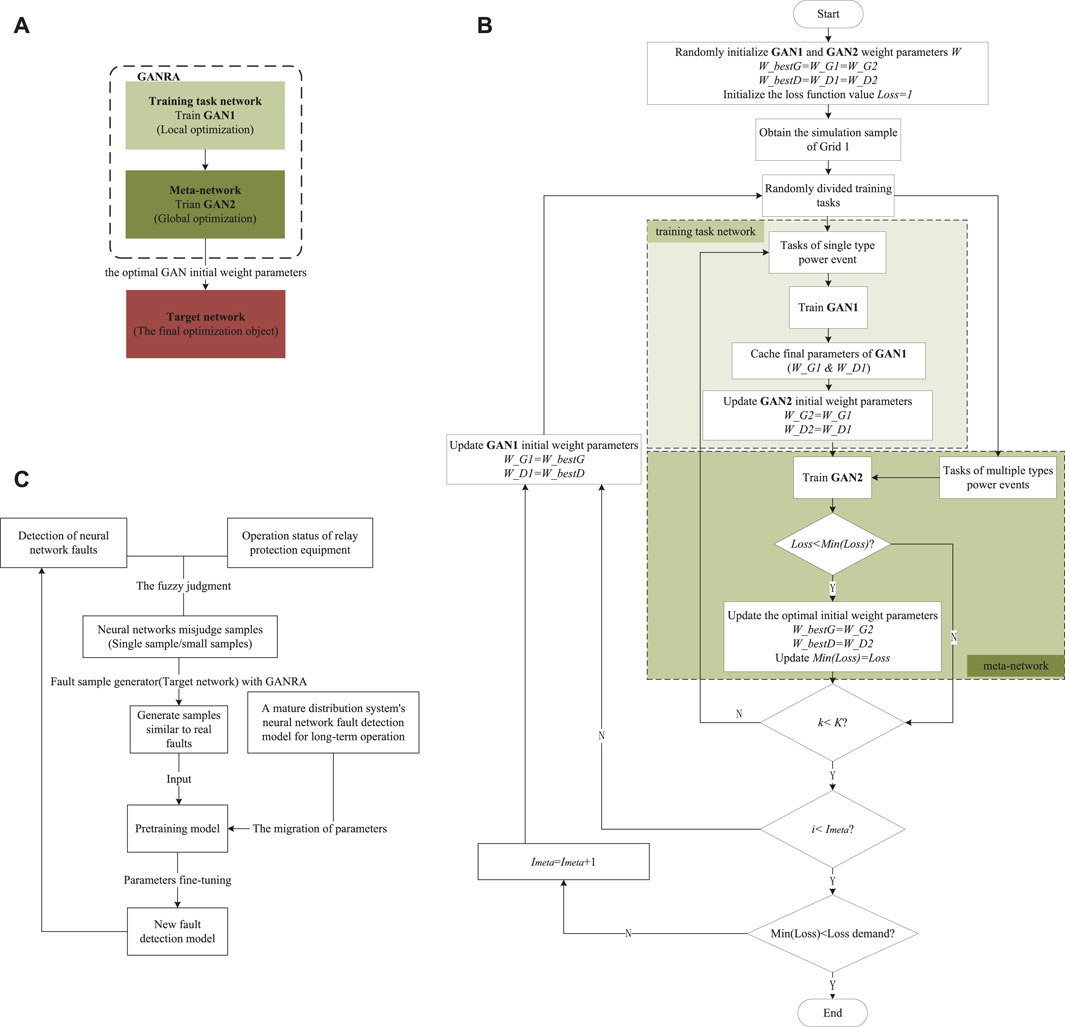
FIGURE 2. (A). The relationship between meta-network, training network, target network and GAN. (B). The algorithm process of GANRA to optimize the initial parameters of the target network. (C). The diagram of practical evolution strategy.

3.1 Meta-network

According to the updated parameters in the training task network, the search direction of initialization parameters with more potential for employment in the future training task is determined. Furthermore, meta-networks directly determine the specific value of the initialization parameters.

The meta-network learning rate ɛ (iteration step) is an adaptive value that changes with the iterations, as shown in Eq. 5.

$\epsilon =a\frac{i}{I_{meta}}+b\left(1-\frac{i}{I_{meta}}\right)(5)$

Where I_meta is the meta-network loop iteration, i is the current meta-network iteration, a and b are adjustable learning rate parameters. a and b decide the parameter update vector of the meta-network. Nichol et al. (2018) shows the learning curves for various loop gradient combinations. The improvement is more significant when using a sum of all gradients in Reptile rather than using just the final gradient in FOMAML. When a=b=1, the parameter update vector of the meta-network is the sum of all iterations’ gradients from the training task network. These two reasons suggest that a=b=1 can benefit from taking many meta-network loop steps.

When multiple training tasks are running in parallel, the weight updating formula of the meta-network layer is shown in Eq. 6.

$\varphi \leftarrow \varphi +\epsilon \frac{1}{N}\sum _{j=1}^N\left({\tilde{\varphi }}_j-\varphi \right)(6)$

Where ϕ are all layer weight parameters of the meta-network, ${\tilde{\varphi }}_j$ are all layer weight parameters obtained by network training of the jth training task in the current meta-network iteration round, N is the number of parallel training tasks used in a meta-network iteration, j is the task network’s number undergoing training in the current meta-network iteration.

Compared with MAML (Wang et al., 2021), First-order MAML (FOMAML), and other meta-learning optimization algorithms, without using gradient or Hesse matrix in the weight update of the meta-network, the Reptile algorithm is faster.

3.2 Training task network

In essence, the training task network is a GAN. And the parameters’ optimization reference direction of the meta-network is obtained through two aspects. One is randomly setting sample tasks with a specified number and categories, i.e., shot and ways, and the other is using the parameters obtained during the training task network after several iterations, i.e., k. Moreover, to ensure the generalization of the meta-network, the training task network uses multi-task parallel training. Finally, the parameters obtained by the training task network are averaged. The above steps are shown in Eq. 6 in section 3.1.

Since GAN is selected as the grid structure of the meta-network, training task network, and target network, the loss function L in the GANRA is defined as the approximate expression $\tilde{V}$ of Eq. 3, as shown in Eq. 7. It can obtain parameter updates and estimate loss values more concretely.

$L=-\tilde{V}=-\left(\frac{1}{m}\sum _{i=1}^m\log \mathrm{D}\left(x_i\right)+\frac{1}{m}\sum _{i=1}^m\log \left(1--\mathrm{D}\left({\tilde{x}}_i\right)\right)\right)(7)$

Where x_i is the ith point sampled in function P_data(x), $\widetilde{x_i}$ is the ith point sampled in function P_G(x), m is the total number of sampling points in the feature distribution of x.

3.3 Generalization and rapidity of initial parameter search

The study takes two rounds of SGD training task network iteration, i.e., K=2, in a meta-network training as an example of the parameter updating process. The initialization parameters of the training task network are shown in Eq. 8.

${\theta }_0=\varphi =\left\{{\theta }_{\text{G}},{\theta }_{\text{D}}\right\}(8)$

Parameters obtained in the next two training rounds are shown in Eqs 9, 10.

${\theta }_1={\theta }_0-\alpha L_0^{\prime }\left({\theta }_0\right)(9)$

${\theta }_2={\theta }_0-\alpha L_0^{\prime }\left({\theta }_0\right)-\alpha L_1^{\prime }\left({\theta }_1\right)(10)$

Where α is the learning rate of the training task network, L′(θ) is the derivative of the training task network’s loss function when the parameter is θ.

The simplified expressions of each function are shown in Eqs 11–14.

$g_k=L_k^{\prime }\left({\theta }_k\right)(11)$

${\theta }_{k+1}={\theta }_i-\alpha g_k(12)$

${\bar{g}}_k=L_k^{\prime }\left({\theta }_0\right)(13)$

${\bar{H}}_k=L_k^{\prime \prime }\left({\theta }_0\right)(14)$

According to Figure 1 in Section 2.1 and the Reptile principle, the parameter descent gradient of the meta-network can be obtained in Eq 15.

$g_{meta}=g_1+g_2={\bar{g}}_1+{\bar{g}}_2-\alpha {\bar{H}}_2{\bar{g}}_1+o\left({\alpha }^2\right)(15)$

According to the derivation of g_meta in Eq. 15, when θ₀ is the initialization parameter of the training task network, the overall average expectation (AvgGrad) of the loss function L’s gradient $\bar{g}$ from a training task network is defined in Eq 16.

$AvgGrad={\mathrm{E}}_{\tau ,i}\left[\bar{g}\right](16)$

The current training sequence of data leads to different training results in the training tasks. Still, due to the random selection of data, the average expectation of θ₀ on the gradient in L is consistent in Eq 17.

$AvgGrad={\mathrm{E}}_{\tau ,1}\left[{\bar{g}}_1\right]={\mathrm{E}}_{\tau ,2}\left[{\bar{g}}_2\right](17)$

Similarly, the expected value of the other part of g_meta is shown in Eq 18.

$AvgGradInner={\mathrm{E}}_{\tau ,\mathrm{1,2}}\left[{\bar{H}}_2{\bar{g}}_1\right]={\mathrm{E}}_{\tau ,\mathrm{1,2}}\left[{\bar{H}}_1{\bar{g}}_2\right](18)$

Then we obtain

$\begin{array}{c}AvgGradInner=\frac{1}{2}{\mathrm{E}}_{\tau ,\mathrm{1,2}}\left[{\bar{H}}_2{\bar{g}}_1+{\bar{H}}_1{\bar{g}}_2\right]\hfill \\ =\frac{1}{2}{\mathrm{E}}_{\tau ,\mathrm{1,2}}\left[\frac{\partial }{\partial {\varphi }_1}\left({\bar{g}}_1\cdot {\bar{g}}_2\right)\right]\hfill \end{array}(19)$

The expected value of g_meta can be obtained as shown in Eq 20.

$\begin{array}{c}\mathrm{E}\left[g_{meta}\right]=2\times AvgGrad\hfill \\ -\alpha \times AvgGradInner+o\left({\alpha }^2\right)\hfill \end{array}(20)$

It shows that the meta-network wants to obtain the same gradient in each training task network’s iteration. This target requires that the initial parameters have generalization. At the same time, the smaller the gradient difference in each iteration of the training task network, the more consistent the search direction of the meta-network to seek the optimal initial parameters and the shortest search path.

3.4 Algorithm implementation

The algorithm process of GANRA to optimize the initial parameters of the target network is shown in Algorithm 1; Figure 2B.

Algorithm 1. GANRA

1) Initialize the weights of the meta-network ϕ₀,

2) Set each hyper-parameter in GANRA,

3) for meta-network iteration rounds i=1,2,…,I_meta do:

4) N tasks of T are sampled,

5) for j=1,2,…,N do:%Train N parallel tasks in the training task network

6) Initialize the network weights of training tasks θ_j=ϕ_i−1,

7) for train task network iteration rounds k=1,2,…,K do:

8) Perform GAN training on task T_j,

9)Obtain the training task network weight θ_j of task T_j,

10) end for

11) end for

12) Update the weights of the meta-network ${\varphi }_i\leftarrow {\varphi }_{i-1}+1/K*\epsilon {\mathrm{\Sigma }}_{j=1}^N({\theta }_j-{\varphi }_i)$

13) end for

The hyper-parameters set in the algorithm include the meta-network iterations I_meta, the number of parallel training tasks N, the training task network iteration rounds K, single task size shot, and task type (or fault type) ways.

4 A practical evolution strategy for neural networks applied to distribution system

4.1 Existing problems

When investigating the fault detection application of neural network in the distribution system, it is found that the transmission lines of the distribution system usually have the following characteristics not conducive to the fault detection application of neural network.

1. The distribution system grid structure is complex and frequently changes, so the training model without continual and timely updating is not applicable.

2. The number of lines in the distribution system is huge, and it is impossible to record fault samples for each branch by installing recording devices. And the types of fault samples recorded are few, mostly single-phase grounding faults. The above reasons result in a small number of recorded waves. In addition, because of low fault current and obscure waveform characteristics, the recorded waves of HIF identified and recorded by subsequent protection devices are rare.

3. The fault characteristics of the distribution system cannot be learned entirely by using samples generated by the simulation model. First, due to the randomness and time-varying nature of the weather and the terrain, it is difficult to determine the fault current and fault types on the line or completely restore the complex factors through modeling. These lead to a truncation error. Second, the neural network is a “black box”. It is unclear if the neural network misses the characteristics of the faults, making it challenging to generate new samples with corresponding tags.

Since the neural network directly learns fault features instead of grid operation rules, the mature fault detection model in the actual grid structure cannot be immediately used in the alternative or changed grid structure. The judgment accuracy of the changed grid structure would be significantly reduced.

4.2 Practical evolution strategy

For applying the neural network fault detection model to practical engineering, the evolution strategy armed with GANRA is designed as the following three stages.

1. Use the GANRA to generate optimal initialization parameters of the misjudgment sample generator.

2. The misclassification sample generator constructs samples with hidden features not learned by the neural network fault detection model. The hidden features are from a few actual misclassification fault samples.

3. The fault detection model trained with a large number of simulation samples or the model in the long-term operation of the distribution system is used as the pre-training model. Deep transfer learning (Bousmalis et al., 2016) is used to transfer the pre-training model to the training model. Then input the generated samples from Step (2) for the parameter fine-tuning training of the training model. A detailed description of the migration strategy is shown in Section 5.5.

The flow of the practical evolution strategy is roughly shown in Figure 2C.

5 Simulation experiment and result analysis

This section analyzes the effect of GANRA on generating HIF samples based on simulation data. Section 5.2 proves the effectiveness of GANRA in the study of initial training parameters with generalization. Moreover, this section observes the learning speed of sample generation and the quality of generated samples. The generated samples are made with the initial parameters obtained by GANRA and tested in the target network. Section 5.3 compares several sample generation algorithms to get their effect on the fault discrimination model generated by CNN under different sample mixing ratios. The algorithms include the conventional GAN with random initial parameters, the conventional GAN with GANRA initial parameters, and Variational Auto-encoders (VAE) (Zhai et al., 2019). It is worth noting that the GANRA in this section optimizes initial parameters from the CNN. Section 5.4 conducts experiments under the influence of different proportions of generated samples on the training accuracy of neural networks. Section 5.5 uses GANRA to find a group of initial parameters based on grid structure 1, then generates samples of grid structure 2 with these parameters and random initial parameters. Finally, Section 5.5 tests the effect of the fault detection model with these training samples. The specific structure composition of the grids can be found in Section 5.1, and the hyper-parameter values used by the GANRA to generate the initial parameters are given in Section 5.3.

5.1 Simulation grid structure and sample composition

A distribution system simulation model is constructed for flexibility in data acquisition, processing and analysis. The simulation sample is taken as the actual sample.

The grid structure of the 10 kV distribution system is shown in Figure 3. The simulation diagram can refer to Supplementary Figure S1. In Figure 3; Figure 4, the symbol “F (⋅)” represents the location of the failure point, the solid line means the overhead line, the dotted line represents the cable line, and every “Load” can be adjusted.

FIGURE 3

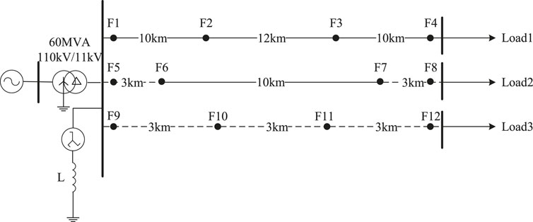
FIGURE 3. Schematic diagram of distribution system grid structure 1.

FIGURE 4

FIGURE 4. Schematic diagram of ring network grid structure 2.

The actual samples used for neural network training and verification, including waveform samples of various faults and normal distribution system conditions, are collected from the fault occurrence point F1. Fifteen thousand nine hundred ninety three fault data are generated for training task extraction and neural network training and testing. This paper mainly studies the situations of HIF. Most of the fault data are HIF data, with a total of 13,438 items. The account of each fault type is shown inTable 1.

TABLE 1

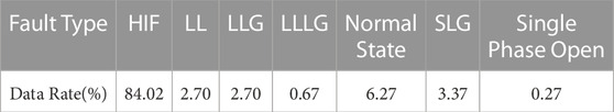
TABLE 1. Proportion of each failure type in grid structure 1.

Where LL represents line-to-line fault (or phase fault), LLG represents line-to-line ground fault (or two-phase ground fault), LLLG represents three lines ground fault (or three-phase ground fault), and SLG represents single-line ground fault (or Normal Single Phase). The common working conditions include load switching, line reclosing, and capacitor switching at the load terminal.

Grid structure 2 is used to verify the generality of the initial parameters generated in Section 5.4. And it is shown in Figure 4, where the classical IEEE 9 node structure model is adopted. The simulation diagram can refer to Supplementary Figure S2. In the experiment, grid structure 2 runs in a way of open loop. Similarly, the collection point of waveform samples for various faults is F1. To simulate the lack of fault detection experience in a new grid structure or system operation mode, it is designed to generate and collect only 4,200 fault data for training task extraction, neural network training, and neural network testing. And among these 4,200 fault data, only 1,440 are high impedance fault data. The account of each fault type is shown in Table 2.

TABLE 2

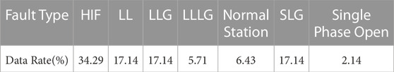
TABLE 2. Proportion of each failure type in grid structure 2.

The use of such a large difference between the ring network and the radial network as a control experiment is mainly to emphasize that even in the case of huge changes in the grid structure, the initial parameters generated by GANRA under the original grid structure still have the ability to assist the new grid structure to generate accurate samples.

The study collects the waveforms of three-phase voltage, three-phase current, zero-sequence voltage, and zero-sequence current in the above simulations and decomposes the signals, respectively. The wavelet decomposition method with a 6 dB parent wavelet extracts the relevant characteristic quantities of wavelet coefficients. Four wavelet coefficients are obtained by three wavelet decomposition. It consists of a three-layer complex wavelet coefficient and one-layer neighboring wavelet coefficient, and thirty-two lines of information can be obtained. Then, by summarizing the high-resolution waveform data in detail and getting the sum of the multiple sampling points, it receives waveform information with thirty-two columns. The formula (Pan, 2019) for the energy relationship between the time domain and frequency domain is shown in Eq 21.

$e_m^n=\sum _{x=1}^X|a_m^2\left(x\right)\cdot \mathrm{\Delta }t|(21)$

Where $e_m^n$ represents the nth pixel block containing time-frequency information of the wavelet coefficient of the corresponding waveform in the mth line of the actual input image sample, a_m(x) represents the sampling amplitude of the xth sampling point of the wavelet coefficient of the corresponding waveform in the mth row, △t is the sampling step, X means that the pixel block contains X sampling points, and each row of 32-pixel blocks contains 32*X amount of sampling point (waveform) information. Figure 5 shows the sample composition of the simulated waveform data obtained by sample processing.

FIGURE 5

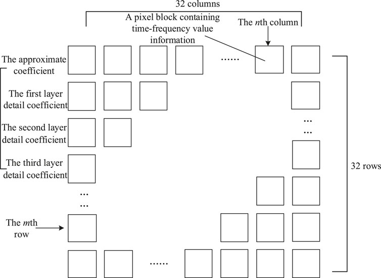
FIGURE 5. Image sample composition schematic diagram.

5.2 Sample generation experiment

A single training task is extracted to conduct GAN training with 1,000 iteration rounds gan_epoch, and the loss values of G and D are obtained respectively, as shown in Figure 6.

FIGURE 6

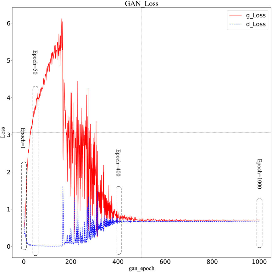
FIGURE 6. Loss chart for a single training mission.

Compare the lines of Figure 6 with the broken line graphs of G and D loss values from the GAN training tasks (Task1, Task2, Task3, and Task4). These tasks use initialization parameters obtained from four different I_meta training of GANRA (as shown in Figure 7). In Figure 7, the training task network’s iteration limit K of the four tasks is 10, and the learning rate of G and D is 0.002. It is found that the G and D loss (g_Loss and d_Loss) of each training task roughly corresponds to the loss trend within the corresponding interval of GAN training rounds in a single training task. Wherein the meta-network iterations I_meta={ 1, 50, 400, 1,000}.

FIGURE 7

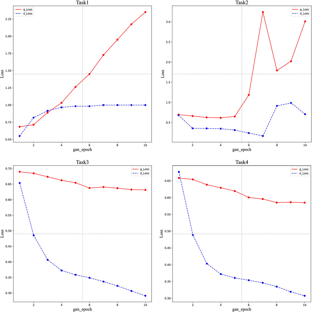
FIGURE 7. Diagram of training task loss under different I_meta.

The hyper-parameter settings of GANRA to the four training tasks in Figure 7 are shown as follows: the number of parallel training tasks N=4, iterations of training task network K=10, adjustable parameters of learning rate of meta-network a =1, b=1, single task size shot =5, and task type ways=7.

The actual samples, the samples generated by the conventional GAN with random initial parameters and the samples generated by the conventional GAN with the optimized initial parameters are compared to study the influence of the initial parameters, the GANRA’s meta-network iterations, and the GAN’s iterations on specific GAN’s generated samples. GANRA generates all the defined initial parameters. The comparison between the actual sample image and the generated sample image is shown in Figure 8. Figures 8A,B compare the sample pictures of HIF generated by the GAN network with and without the optimized initialization parameters. Both are trained for 400 rounds. It can be found that the GAN with the optimized initialization parameters can preliminarily generate images with actual image sample features. This result is obtained with the GAN iterations epoch=400 and 50 rounds of meta-network training. And it reflects that GANRA can accelerate GAN’s collection of image features. Figures 8C, D compare the results of more rounds of GAN training based on Figures 8A, B. In this case, the GAN assisted by GANRA can generate a noiseless image sample, while some of the image samples generated by general GAN still have high noise. This phenomenon indicates that GANRA can reduce the noise of the generated samples. Figures 8E, F provide a comparison diagram between 950 GAN epochs generation sample with 1000 GANRA meta-network iterations and the original sample. The generated sample is almost consistent with the actual one, and the research results show this method is promising. However, contrasting the GANRA-assisted sample generation in Figures 8C, D with Figures 8E, F, the initialization parameters generated by multiple iterations of the meta-network have a specific “saturation value”. In other words, the GAN’s iterations for a particular task will not be further reduced. The quality of the generated samples and the GAN’s iterations to generate quality-compliant samples will not change significantly in the case of a sharp increase in I_meta. The above experimental results are limited by the expectation of GANRA parameters’ generalizability. The detail of Figure 8 can refer to the Supplementary Material S1

FIGURE 8

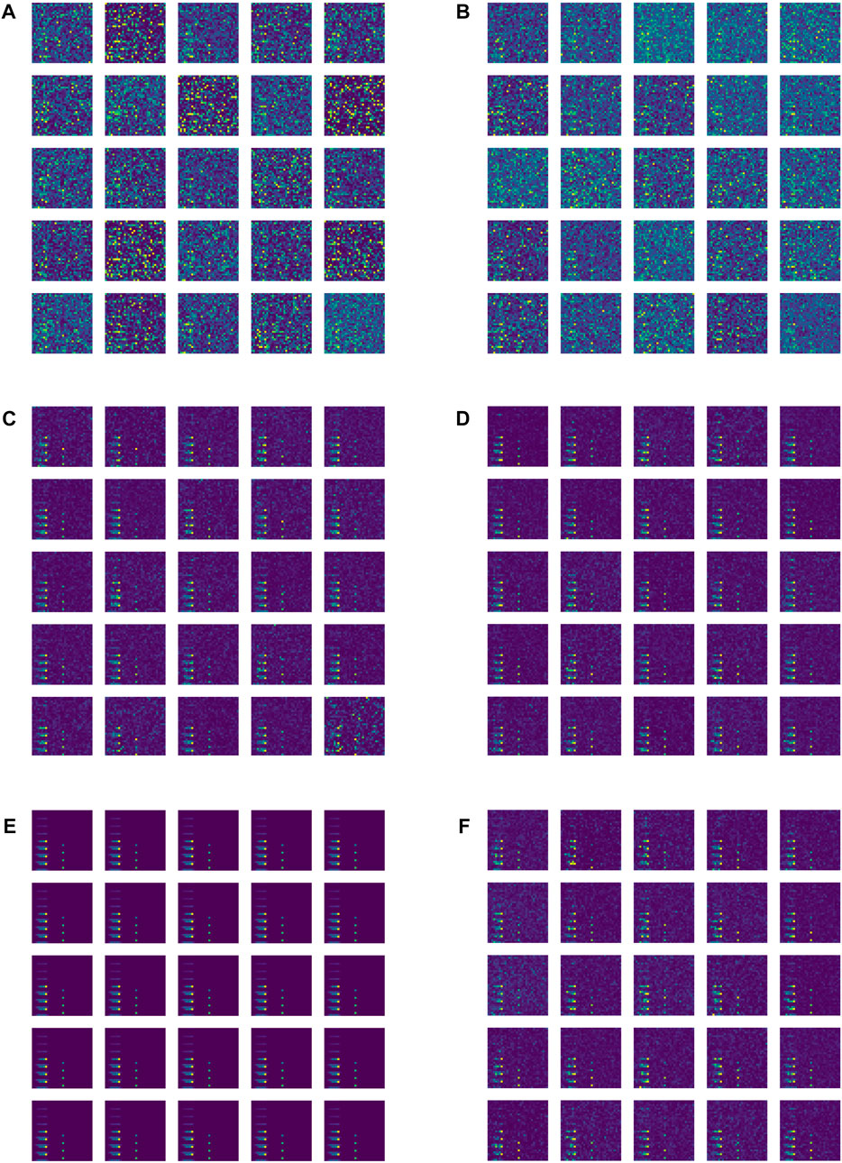
FIGURE 8. The actual sample of high resistance ground fault and the generated sample diagram under different experimental conditions. (A) GAN, epoch=400 (B) GANRA, I_meta=50, epoch=400. (C) GAN, epoch=960. (D) GANRA, I_meta=50, epoch=950. (E) Original samples. (F) GANRA, I_meta=1,000, epoch=950.

5.3 Experiments on the similarity between samples generated by several generation methods and the actual samples

The settings of GANRA’s hyper-parameters and the base model used in fault detection in Sections 4.3, 4.4, and 4.5 are the same. The hyper-parameters of GANRA are set as follows: the meta-network iteration rounds I_meta=1,000, the number of parallel training tasks N=4, the training task network iteration rounds K=10, the meta-network learning rates a =1, b=1, the single task size shot=35, and the task type ways=1. Only the binary classification of the HIF and non-HIF faults is performed in this study. And the HIF recognition accuracy in this study is used to reflect the similarity between the generated HIF samples and the actual samples. The training set comprises the generated samples from different generation methods of grid structure 1, and the testing set contains the simulated samples (called actual samples) of grid structure 1.

A CNN consisted of three convolutional layers and two fully connected layers is selected for the basic model settings used in fault detection. The Relu function is used as the activation function. The learning rate α=0.001, iteration epoch=20, and single training scale batch_size=66. In this section, the iterations of GAN with initial parameters generated by the GANRA and with random initial parameters are 500 rounds. The VAE sample generation model in the study refers to the classical model (Pan, 2019).

It can be seen from Table 3 that the samples generated by GANRA and the samples generated by conventional GAN both have a high degree of similarity with the actual sample. And several experimental phenomena show that the recognition accuracy does not fluctuate much with different GAN initial parameters. At the same time, the recognition accuracy of VAE-generated samples jumps between 55% and 100% during the experiment. The study indicates that VAE learns some features of actual samples accurately but lacks robustness in other areas. By contrast, GANRA knows these features of samples in a stable and satisfactorily precise way. However, compared with the network that only uses GAN to learn and generate HIF samples, the generated HIF samples are slightly less reductive than the actual samples because it emphasizes the generalization of all fault initialization parameters instead of the optimum of current parameters.

TABLE 3

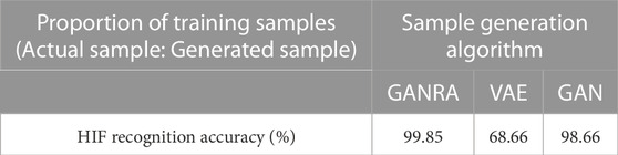
TABLE 3. The similarity between the samples generated by different methods and the actual samples of grid 1.

5.4 Influence experiment of sample proportion on training accuracy

The testing set includes 2,100 actual samples from grid structure 2, and the training set includes both the actual and the samples generated by GANRA. The proportions of mixed samples are shown in Table 4. In addition, the data from the training set and testing set are not coincidental, and the proportions between the training set and testing set are always kept at a 1:1 ratio. The effect of different sample structures on the fault detection accuracy of grid structure 2 is shown in Table 4.

TABLE 4

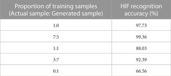
TABLE 4. Influence of different sample composition on fault detection accuracy of grid 2.

As seen from Table 4, the generated samples supported by GANRA achieve optimal performance in the experiments. Its HIF recognition accuracy is 99.36% when the proportion of training samples (actual sample: generated sample) is 7:3.

5.5 Fault detection experiments under changing conditions of the grid structure

According to the practical evolution strategy proposed in Section 4.2, relevant simulation experiments are carried out on the grid structure 2 with several samples. In the simulation experiment setting, the initial GAN parameters generated by GANRA through grid structure 1 are applied to the generation of small samples of grid structure 2 to show whether the GANRA focuses on predicting initialized parameters on future tasks.

The fault pre-training model adopted is the basic CNN model mentioned in Section 5.2. The migration parameters used in the new neural network are obtained after training the actual sample from grid 1. On this basis, a mixture of samples is used to prepare the fine-tuned parameters of the new fault detection model. The mixed samples include generated samples and a small number of actual samples. The specific transfer learning strategies are as follows: first, the top-level 1 of the actual model is turned into the top-level 2 of the new model, and this new model is more suitable for the current training data; second, freeze the parameter training of the bottom and middle layers of the new model, and train only the top layer 2; third, the parameter training of the bottom layer and middle layer 1 of the new model is frozen, and then the top layer 2 and middle layer 2 are trained simultaneously. The corresponding transfer learning strategy is shown in Figure 9. The box is filled with grey layers for the parameters to be trained in the specified step.

FIGURE 9

FIGURE 9. Transfer learning strategy.

The proportion of mixed training samples is 7:3 based on Section 5.4, which can make the recognition of HIF relatively more accurate. The specific experimental control group is set as follows.

1. Train the new neural network with the actual sample of grid 2.

2. The actual sample of grid 2 is used to fine-tune the parameters from the neural network of grid 1.

3. The generated sample are mixed with fine-tuning the parameters from the neural network of grid 1 and the actual sample of grid 2.

4. The generated samples of grid 2 are used to fine-tune the parameters from the neural network of grid 1.

5. The neural network of grid 1 detects test samples of grid 2.

The influence of the different proportions of models’ fine-tuning and training samples on HIF recognition accuracy of grid structure 2 is shown in Table 5.

TABLE 5

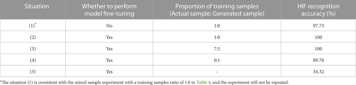
TABLE 5. HIF recognition accuracy in grid structure 2 under different training conditions.

The comparison between situations (1) and (2) shows that neural network transfer learning can effectively improve the identification accuracy of HIF. By the comparison of (2), 3, and 4, it is easy to find that using appropriate mixed samples to increase the training sample size is feasible when there are few fault samples in the new grid structure. This method will not decrease the fault identification accuracy. However, a large proportion of generated samples will decrease the identification accuracy. The comparison between cases (2) and (5) shows that the parameter fine-tuning in the new grid structure is feasible. It can significantly improve fault identification accuracy. Therefore, the practical evolution strategy of neural networks for distribution systems is effective. It can optimize the utilization of neural networks in power system fault detection.

6 Conclusion

This paper proposes a GAN evolution strategy based on the Reptile algorithm to solve practical problems such as small HIF samples and network structure changes in distribution systems. The validity, generalization, and speed of GANRA are verified by mathematics and simulation. The sample generated by the neural network evolution strategy helps solve some problems (like a shortage of reliable training data and faults with obscure characteristics) existing in practical applications through the auxiliary neural network fault detection model. Furthermore, GANRA generates the initial parameters of GAN through indirect gradient calculation and completes a general optimization of initial parameters. GANRA can generate samples with better quality faster than GAN, but when the number of iterations tends to a certain upper limit, the quality of samples generated by GAN is better than that of GANRA because of GANRA parameters’ generalizability. And the quality of samples generated by GANRA is usually better than that of VAE. This algorithm effectively reduces the computing time, sample size and the number of learning iterations required to generate samples in different tasks and grid structures in the future.

For the electrical field, considering the requirements of timeliness and stability of fault judgment in engineering practice, such a study can be done by presenting the process of GANRA optimization of initial parameters in a dynamic and online way. In addition, the influence of other GAN algorithm variants on parameter iteration can be explored. For example, a tagged grid structure emphasizing classification ability can be considered. That is for enhancing the training ability in the category of samples with significant differences. Then, the research can extend this ability to other categories of fault identification.

Data availability statement

The raw data supporting the conclusion of this article will be made available by the authors, without undue reservation.

Author contributions

HB and WJ were responsible for providing the study idea, experiment design, experiment execution, result analyses, and manuscript draft. ZD were responsible for supervision, review, and funding acquisition. WZ, XL, and HL were responsible for providing part of experiment execution. All authors contributed to the article and approved the submitted version.

Funding

This work was supported by the Science and Technology Project of the China Southern Power Grid (GDKJXM20198281). The funder was not involved in the study design, collection, analysis, interpretation of data, the writing of this article, or the decision to submit it for publication.

Conflict of interest

Author HB was employed by China Southern Power Grid. XL was employed by the Zunyi Power Supply Company of Guizhou Power Grid.

The remaining authors declare that the research was conducted in the absence of any commercial or financial relationships that could be construed as a potential conflict of interest.

Publisher’s note

All claims expressed in this article are solely those of the authors and do not necessarily represent those of their affiliated organizations, or those of the publisher, the editors and the reviewers. Any product that may be evaluated in this article, or claim that may be made by its manufacturer, is not guaranteed or endorsed by the publisher.

Supplementary material

The Supplementary Material for this article can be found online at: https://www.frontiersin.org/articles/10.3389/fenrg.2023.1180555/full#supplementary-material

References

Amir, H., and Gandomi, L. M. P. Z. (2022). Reptile search algorithm (rsa): A nature-inspired meta-heuristic optimizer. Expert Syst. Appl. 191, 116158. doi:10.1016/j.eswa.2021.116158

CrossRef Full Text | Google Scholar

Bousmalis, K., Trigeorgis, G., Silberman, N., Krishnan, D., and Erhan, D. (2016). “Domain separation networks,” in Annual Conference on Neural Information Processing Systems 2016, Barcelona, Spain, December 5-10, 2016, 343–351.

Google Scholar

Finn, C., Abbeel, P., and Levine, S. (2017). “Model-agnostic meta-learning for fast adaptation of deep networks,” in Proceedings of the 34th International Conference on Machine Learning, Sydney, August 6 - 11, 2017, 1126–1135.

Google Scholar

Flauzino, R. A., Ziolkowski, V., and Silva, I. N. D. (2006). “Using neural network techniques for identification of high-impedance faults in distribution systems,” in 2006 IEEE/PES Transmission and Distribution Conference and Exposition: Latin America, Caracas, August, 15-18, 2006, 1–5.

CrossRef Full Text | Google Scholar

Geng, J., Wang, B., Dong, X., and Dominik, B. (2013). Analysis and detection of high resistance grounding fault in neutral effective grounding distribution network. Power Syst. autom. 37, 85–91.

Google Scholar

Goodfellow, I. J., Pouget-Abadie, J., Mirza, M., Xu, B., Warde-Farley, D., Ozair, S., et al. (2014). “Generative adversarial nets,” in Advances in Neural Information Processing Systems 27: Annual Conference on Neural Information Processing Systems 2014, Montreal, Quebec, Canada, December 8-13 2014, 2672–2680.

Google Scholar

Li, Y., Zhang, S., Hu, R., and Lu, N. (2020). A meta-learning based distribution system load forecasting model selection framework. Appl. Energy 294, 116991. doi:10.1016/j.apenergy.2021.116991

CrossRef Full Text | Google Scholar

Mo, S., Cho, M., and Shin, J. (2020). Freeze discriminator: A simple baseline for fine-tuning gans. Available at: https://arxiv.org/abs/2002.10964 (Accessed February 25, 2020).

Google Scholar

Nichol, A., Achiam, J., and Schulman, J. (2018). On first-order meta-learning algorithms. Available at: https://arxiv.org/abs/1803.02999 (Accessed March 8, 2018).

Google Scholar

Pan, X. (2019). “Research on high resistance grounding fault detection of distribution lines,”. Thesis (Changsha: Hunan university).

Google Scholar

Salomonsson, D., Söder, L., and Sannino, A. (2007). “An adaptive control system for a dc microgrid for data centers,” in Conference Record of the 2007 IEEE Industry Applications Conference Forty-Second IAS Annual Meeting, New Orleans, LA, USA, September 23-27, 2007 (IEEE), 2414–2421. doi:10.1109/07IAS.2007.364

CrossRef Full Text | Google Scholar

Wan, Q., and Zhao, L. (2018). “A novel fault section location method for small current grounding fault based on hilbert-huang transform with wavelet packet transform preprocessing,” in 2018 11th International Conference on Intelligent Computation Technology and Automation (ICICTA), Changsha, September 22-23, 2018, 365–370. doi:10.1109/ICICTA.2018.00089

CrossRef Full Text | Google Scholar

Wang, F., Chai, G., Li, Q., and Wang, C. (2022). Small sample malware classification method based on parameter optimization meta-learning and difficulty sample mining. J. Wuhan Univ. Nat. Sci. 68, 17–25. doi:10.14188/j.1671-8836.2021.2008

CrossRef Full Text | Google Scholar

Wang, J. (2020). “Research on cloud fault diagnosis method of Service robot based on mixed samples,”. Thesis (Jinan: Shandong university).

Google Scholar

Wang, X., Yu, Z., Shi, B., Bao, Z., Qian, H., and Zhao, Y. (2021). Small sample data generation algorithm based on meta-learning. Comput. Syst. Appl. 30, 161–170. doi:10.15888/j.cnki.csa.008063

CrossRef Full Text | Google Scholar

Wang, Z., and Zhang, B. (2021). A review of generative adversarial networks. J. Netw. Inf. Secur. 7, 68–85.

Google Scholar

Xi, J., Pei, X., Song, W., Xiang, B., Liu, Z., and Zeng, X. (2021). Experimental tests of dc sfcl under low impedance and high impedance fault conditions. IEEE Trans. Appl. Supercond. 31, 1–5. doi:10.1109/TASC.2021.3065886

CrossRef Full Text | Google Scholar

Xie, J. (2019). “Modeling and debugging of PSCAD for the main grid of power transmission from west to East of China Southern Power Grid,”. Thesis. Guangzhou, China: (South China University of Technology).

Google Scholar

Xu, R., Liu, B., Zhang, K., and Liu, W. (2022). Model independent element learning algorithm based on bayesian weight function. Comput. Appl., 1–5. doi:10.11772/j.issn.1001-9081.2021040758

CrossRef Full Text | Google Scholar

Ye, J., Chu, F., and Wu, Y. (2016). Fault type identification of distribution network based on wavelet packet and improved neural network. Sci. Technol. innovation Appl. 1, 18–19.

Google Scholar

Zhai, Z., Liang, Z., Zhou, W., and Sun, X. (2019). A review of variational autoencoder models. Comput. Eng. Appl. 55, 1–9.

Google Scholar

Zhang, H., and Su, L. (2022). Zero-sample image recognition for variational autoencoder combined with knowledge graph. Comput. Eng. Appl., 1–10. doi:10.3778/j.issn.1002-8331.2106-0430

CrossRef Full Text | Google Scholar

Zhang, J. (2018). “Research on intelligent identification method of high resistance grounding fault in distribution network,”. Thesis (Fuzhou: Fuzhou university).

Google Scholar