Overload capacity analysis of extra high voltage AC XLPE submarine cable

When submarine cable line fails or other lines need load transfer, it often suffers from emergency ampacity that exceeds the steady-state ampacity. The layout environment of the submarine cable is always complex and changeable, and the overload capacity of the submarine cable in different layout environments is also different. Therefore, it is necessary to analyze the overload capacity of the submarine cable. In this paper, a coupled multi-physical field model by finite element method is established for AC 500 kV XLPE extra high voltage submarine cable in landing section, which is the ampacity bottleneck section of the whole line. The overload capacity of submarine cable in two typical layout environments which are direct buried and within pipeline is analyzed. The results show that the overload capacity of submarine cable in the direct buried environment is much higher than that in the pipeline environment. The allowable emergency time in the direct buried environment is 2–3 times that of the pipeline environment under the same condition. In the two typical layout environments, when the emergency current are 2500 A and 3500 A, the ratio of the emergency time allowed to run in the direct buried environment to that in the pipeline environment is about 5 times under the same initial capacity. The proposed model can provide a reference for dynamic capacity control of the extra high voltage submarine cable.

1 Introduction

For extra high voltage (EHV) submarine cable transmission project is a key component of island power supply, offshore wind power new energy grid connection and other cross-sea interconnection projects. How to ensure the economic and rational operation of EHV submarine cable line is the key problem to be solved urgently for the stable operation of offshore electrical engineering (Lv et al., 2014; Liang et al., 2019; Guo et al., 2020).

Conductor temperature and ampacity are the two most important operating parameters of submarine cable. The maximum allowable operating temperature of EHV submarine cable conductor is 90°C (Bian et al., 2019; Hu et al., 2019). The cable core temperature determines the ampacity of the submarine cable, and the ampacity in the case of the cable core temperature reaches 90°C is called the steady-state ampacity of the submarine cable. In practice, submarine cables rarely operate under a constant load for a long time, but respond dynamically according to the actual load changes (Lei et al., 2012; Duraisamy et al., 2018). Therefore, during the operation of the submarine cable line, it is not only necessary to accurately calculate the steady-state ampacity of the submarine cable, but also to conduct analysis on the emergency ampacity (Lin et al., 2021).

At present, the main methods to calculate the ampacity of submarine cables are the thermal circuit method (TCM) based on IEC 60287 standard and the multi-physical field coupling simulation method based on finite element method (FEM) (Hu et al., 2019). References (Lu et al., 2020) and (Zhang et al., 2020) analyzed the ampacity of a 220 kV three-core cross-linked polyethylene (XLPE) submarine cable in different layout environments by establishing the finite element simulation model. Reference (Hu et al., 2019) used a three-dimensional multi-physical field coupling simulation model to analyze the improvement of the ampacity of a 500 kV XLPE submarine cable by different cooling methods. The transient thermal circuit model of 500 kV oil-filled submarine cable is constructed to analyze the overload capacity of submarine cable in different layout environments in (Chen et al., 2021).

When the submarine cable line fails or other lines need to transfer load, it often needs to suffer from the emergency load current that exceeding the steady-state ampacity of the submarine cable. Therefore, it is of great significance to calculate and analyze the overload capacity of submarine cables in engineering (Lin et al., 2021). Previous studies mainly focus on the calculation and analysis of the steady-state ampacity of submarine cables, but lack of research on the overload capacity.

The submarine cable landing section is the ampacity bottleneck section of the whole line. In this paper, the overload capacity of 500 kV AC XLPE EHV submarine cable landing section in the typical layout environment is studied (Duraisamy et al., 2018). Firstly, the electromagnetic-thermal-fluid field coupling simulation model by FEM for the EHV submarine cable is established. Then the steady-state temperature of the EHV submarine cable in different layout environments and operating ampacities is studied, and the overload capacity of submarine cable is further calculated and analyzed. Finally, the maximum allowable emergency time of different emergency ampacity imposed on the submarine cable is determined.

2 Finite element simulation model

In this paper, a 500 kV AC XLPE submarine cable model already in operation in China is taken as the main research object. The submarine cable structure is shown in Figure 1, and the specific material parameters are given in Table 1. The main structure of the 500 kV AC XLPE submarine cable contains copper conductor, conductor shield, insulation layer, shielding layer, metal sheath and outer sheath (Liu et al., 2020).

FIGURE 1

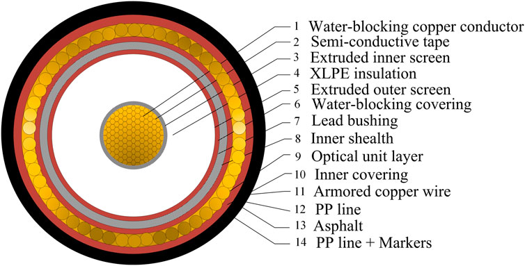
FIGURE 1. Structure of the submarine cable.

TABLE 1

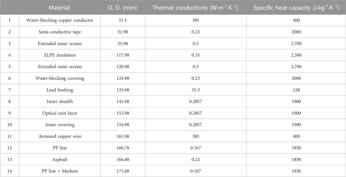
TABLE 1. Material parameters of the submarine cable.

The finite element model of EHV submarine cable mainly includes magnetic field module and heat transfer module. The governing equations of the electromagnetic-thermal physical fields can be written as

${\rho }_{\mathrm{v}}{C}_{\mathrm{p}}\frac{\partial T}{\partial t}+{\rho }_{\mathrm{p}}{C}_{\mathrm{p}}v\cdot \nabla T+\nabla \cdot \left(-k\nabla T\right)=\mathit{J}\cdot \mathit{E}(1)$

where ρ_v is the material density, C_p is the material specific heat capacity, T is the temperature, t is the time, k is the heat transfer coefficient, v is the flow rate, J is the current density, and E is the electric field intensity.

In the finite element model, the copper conductor is set as a single-core coil, and the current through the conductor is set as I. For copper material, the resistivity is not a fixed value, and its resistivity is positively correlated with the temperature. When the temperature is increased, the value of the resistivity is also increased. The linear resistivity model can better reflect the various of the resistance with temperature, and the bidirectional coupling between electromagnetic field and heat transfer field can be realized in the finite element model of EHV submarine cable. Its expression can be written as (Zhang et al., 2016)

$\sigma \left(T\right)=\frac{1}{{\rho }_0\left(1+\alpha \left(T-T_{\text{ref}}\right)\right)}(2)$

where σ is the conductivity, ρ₀ is the reference resistivity, α is the temperature coefficient of resistivity, and T_ref is the reference temperature.

The governing equation of the heat transfer physical field is

${\rho }_v{C}_p\left(\frac{\partial T}{\partial t}+v\cdot \nabla T\right)+\nabla \cdot \left(-k\nabla T\right)=Q(3)$

where Q is the electromagnetic loss.

The boundary conditions of the submarine cable for heat transfer can be classified into three types. The lower boundary of the model is far away from the cable, and the influence of cable heating on the temperature of the lower boundary can be ignored. In the finite element model of the landing section, the lower boundary temperature is taken as 281.15 K. Its expression can be written as (Liang et al., 2007; Duan et al., 2014; Hao et al., 2017).

$T\left(x,y\right){|}_{\mathrm{\Gamma }}=f\left(x,y\right){|}_{\mathrm{\Gamma }}=281.15\mathrm{K}(4)$

The left and right boundaries of the model are set to be thermally insulated, and the expression can be written as

$-k\frac{\partial T}{\partial n}{|}_{\mathrm{\Gamma }}=f\left(x,y\right){|}_{\mathrm{\Gamma }}=0(5)$

The upper boundary of the model is the convective heat transfer boundary with the air, and the expression can be written as

$-k\frac{\partial T}{\partial n}{|}_{\mathrm{\Gamma }}=h\left(T-T_{\mathrm{f}}\right){|}_{\mathrm{\Gamma }}(6)$

The air convection heat transfer coefficient h is generally in the range of 5–25 W‧m⁻²‧K⁻¹, and 8 W‧m⁻²‧K⁻¹ is taken in the model (Liu et al., 2020). The external boundary temperature T_f is taken as 26°C, and the soil thermal conductivity of the landing section k of 0.8 W‧m⁻²‧K⁻¹ is taken in the model (Chen et al., 2021).

There are two main layout methods of submarine cable in the landing section: direct burial in soil and pipeline laying. According to the cable design standard for power engineering GB 50217-2018, the burying depth of the electrical cable should be deeper than 0.7 m (Cable design standard for power, 2018). Therefore, in the model, the burying depth of the submarine cable in the landing section is set as 2 m for these two layout methods. Since the cable spacing in the landing section should not be too long, the horizontal spacing and longitudinal spacing of the cables are both taken as 0.4 m. In order to simulate the layout environment of landing section, the soil area should be as large as possible to avoid the influence of boundary conditions on the simulation results. The lower boundary of the model is 20 m away from the lower submarine cable, and the left and right boundaries of the model are 15 m away from the submarine cable. The environmental parameters of the landing section of the submarine cable are shown in Table 2 (Qiu, 2013; Zhang et al., 2016).

TABLE 2

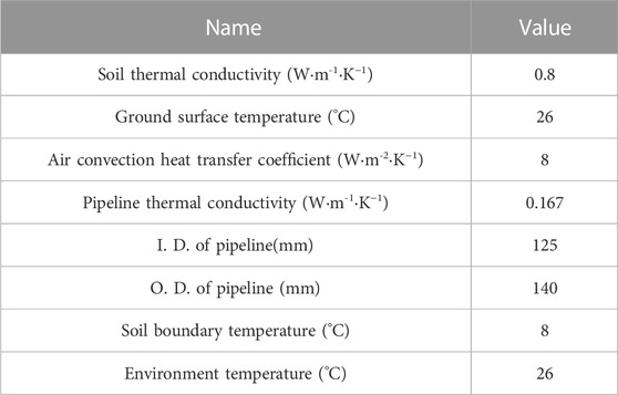
TABLE 2. Landing environment parameters.

It should be noted that the narrow space between the surface of the submarine cable and the inner surface of the pipeline is air, in which the heat transfer mode also includes thermal convection and thermal radiation. However, due to the limited volume of fluid in the narrow space of the pipeline environment, the heat transfer mode of the pipeline is assumed to be closer to heat conduction in this model. The material of the pipeline is PVC.

The topological structure of submarine cable in two different layout environments is shown in Figure 2. In the two layout environments, the geometric model of the landing section of the submarine cable is regular. Therefore, the adaptive triangular grid with strong adaptability and fast division is selected.

FIGURE 2

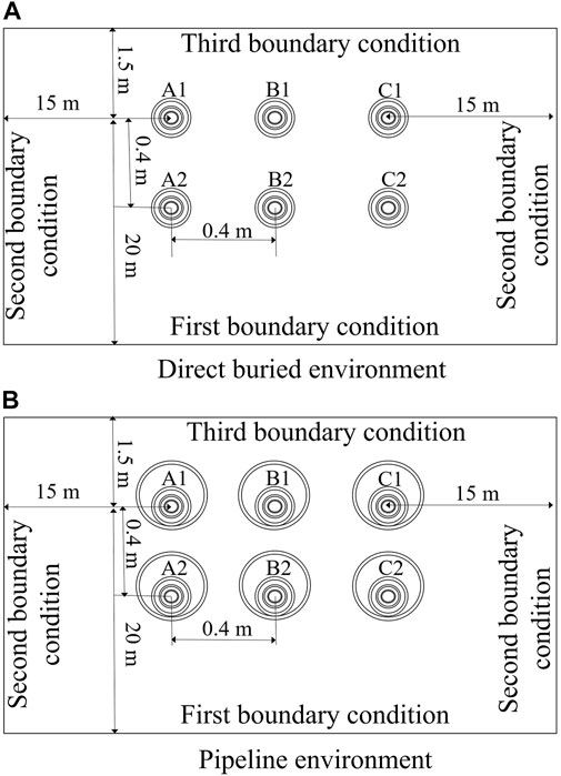
FIGURE 2. Simulation topological structure of landing section of the submarine cable: (A) Direct buried environment, (B) Pipeline environment.

The grid division result of the submarine cable is shown in Figure 3. More accurate solution always can be achieved with smaller meshes, but it will slow down the calculation speed. The part of the submarine cable has a relatively small structure size and a large temperature gradient, so the grid division is fine. The area of the soil part is large and the overall change of the temperature gradient is small, so the grid division is coarse.

FIGURE 3

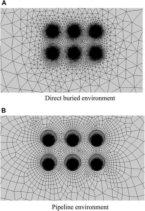
FIGURE 3. Local grid quality map of landing section of the submarine cable: (A) Direct buried environment, (B) Pipeline environment.

3 Results and discussion

3.1 Calculation of the steady-state ampacity

In the two layout environments, when the working temperature of the cable core at the landing section of the submarine cable reaches 90°C, the temperature distribution of the submarine cable and the surrounding soil is shown in Figure 4. It can be seen that the temperature of the mesophase submarine cable conductor is the highest, followed by the left and right phases, and the temperature change is more obvious in the area near the submarine cable. In the direct buried environment, the cable core temperature of phase A and phase C is 3.86°C lower than that of phase B. In the pipeline environment, the temperature of phase A and phase C cable core is 5.4°C lower than that of phase B cable core. Therefore, in the subsequent study, the temperature of the phase B submarine cable core is selected as the research object.

FIGURE 4

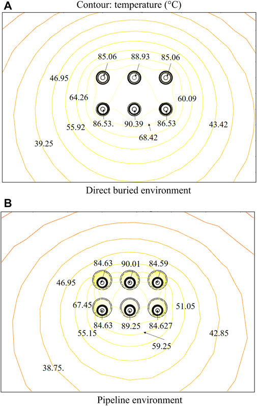
FIGURE 4. Temperature distribution of landing section of the submarine cable: (A) Direct buried environment, (B) Pipeline environment.

The validity of the FEM model is estimated by the TCM. The equivalent thermal circuit model of submarine cable is shown in Figure 5 (Liu, 2020). θ_c is the working temperature of the cable core; θ₀ is the environment temperature, which is taken as 26°C in the model; T₀, T₁, T₂, T₃, and T₄ respectively represent the thermal resistance of the inner shield, insulation layer, inner lining layer, outer coating layer and outer medium layer of the submarine cable per unit length. λ₁ is the ratio of metal sheath loss to conductor loss, λ₂ is the ratio of armor loss to conductor loss, W_c is the conductor loss per unit length of cable, and W_d is the dielectric loss per unit length of cable.

FIGURE 5

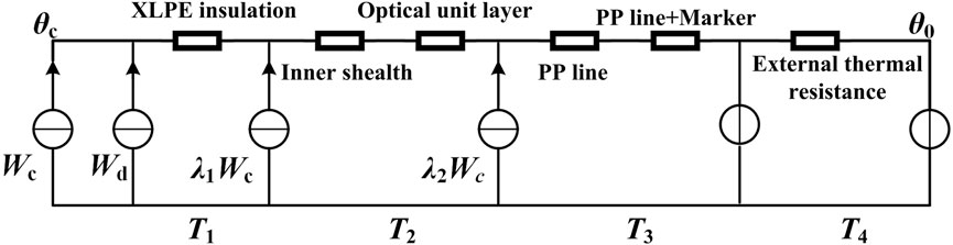
FIGURE 5. Schematic diagram of equivalent thermal circuit model of the submarine cable.

The formula for calculating the steady-state ampacity of the submarine cable can be written as (IEC 60287-1-1, 1994; IEC 60287-1-2, 1994).

$I=\sqrt{\frac{\Delta {\theta }_{\mathrm{c}}-W_{\mathrm{d}}\left[0.5T_1+n\left(T_2+T_3+T_4\right)\right]}{R\cdot T_1+nR\left(1+{\lambda }_1\right)T_2+nR\left(1+{\lambda }_1+{\lambda }_2\right)\left(T_3+T_4\right)}}(7)$

where I is the ampacity the submarine cable, n is the number of submarine cable cores, taking 1 in this paper, R is the resistance of the copper conductor of the submarine cable core, Δθ_c is the difference between the temperature of the copper conductor of the cable core and the environment temperature.

The steady-state ampacity of the bottleneck section of the submarine cable in different layout environments is calculated by the FEM and TCM, and the results are shown in Table 3. It can be seen that when the submarine cable in the landing section is laid in the pipeline environment, the steady-state ampacity is about 100 A lower than that of the direct buried environment. The ampacity of submarine cable in landing section is 1276 A calculated by the FEM and 1,399.5 A calculated by the TCM, with a relative error of 8.82%. The ampacity of submarine cable in landing section is 1170 A calculated by the FEM and 1,219.2 A by the TCM, with a relative error of 4.04%. The results of the two models are in good agreement, indicating that the calculation result of FEM model has a good accuracy. It can be seen that the ampacity calculated by the TCM is always lower than that calculated by the FEM. This is mainly because that in the calculation of TCM, we have considered the dielectric loss caused by the heating of the wire core, the loss caused by the metal sheath and armor part. However, in the calculation of FEM, we only considered the heating of the cable core.

TABLE 3

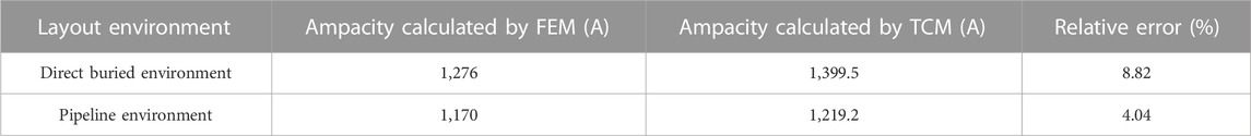
TABLE 3. Comparison of the calculation results of steady state ampacity.

3.2 Calculation of the emergency ampacity

During normal operation, the submarine cable is not always in a steady-state ampacity. When the temperature of the cable core does not reach the upper limit value, the ampacity that exceeding the steady-state ampacity of submarine cable can be applied for a short time (Wang et al., 2013; Zhuang et al., 2014; Lin et al., 2018; Niu et al., 2018). Based on this, combined with the actual operation situation of the submarine cable, the maximum overload operation time is analyzed by using the established finite element multi-physical field coupling simulation model of the submarine cable under different initial ampacity and different emergency ampacity.

When the initial ampacity of the submarine cable is 1000 A, 1050 A and 1100 A respectively, the temperature of the submarine cable core is shown in Table 4. It can be seen that when the initial ampacity is the same, the temperature of the submarine cable core in direct buried environment is about 5°C lower than that of the pipeline environment.

TABLE 4

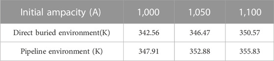
TABLE 4. Steady-state temperature of the cable core under different initial ampacities

When the landing section of the submarine cable is in the direct buried environment, and the initial ampacities are 1000 A, 1050 A and 1100 A respectively, the temperature change of the cable core under different emergency ampacities is shown in Figure 6. It can be seen that when the emergency ampacity is the same, the emergency time decreases with the initial ampacity. With the increase of the emergency ampacity, the allowed emergency time for the cable core to reach the limited temperature (363.15 K) decreases gradually under the three different initial ampacities.

FIGURE 6

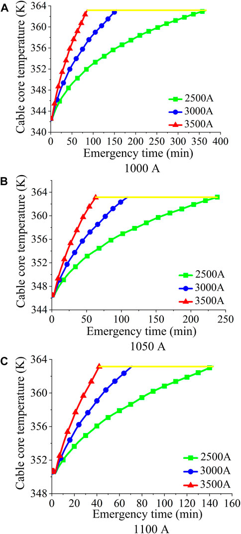
FIGURE 6. Emergency time for different initial ampacities in direct buried environment: (A) 1000 A, (B) 1050 A, (C) 1100 A.

When the landing section of the submarine cable is in the pipeline environment, and the initial ampacities are 1000 A, 1050 A and 1100 A respectively, the temperature change of the cable core under different emergency ampacities is shown in Figure 7. It can be seen that when the emergency ampacity is the same, the emergency time decreases with the initial ampacity. With the increase of the emergency ampacity, the allowed emergency time for the cable core to reach the limited temperature (363.15 K) decreases gradually under the three different initial ampacities.

FIGURE 7

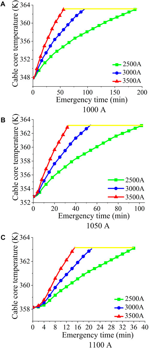
FIGURE 7. Emergency time for different initial ampacities in pipeline environment: (A) 1000 A, (B) 1050 A, (C) 1100 A.

For the two different layout environments, the calculated emergency time is shown in Table 5. When the initial ampacities are 1000 A and 1050 A, the emergency time in the case of direct buried environment is about 2 times that of pipeline environment. When the initial ampacity is 1100 A, the emergency time in the case of direct buried environment is about 3 times that of pipeline environment. When the initial ampacity is 1000 A, the temperature of the submarine cable core reaches the maximum allowable temperature after 366, 156, and 86 min respectively at the emergency ampacities of 2500 A, 3000 A and 3500 A in the direct buried environment. The cable core temperature reaches the maximum allowable working temperature after 190, 95, and 57 min at the emergency ampacities of 2500 A, 3000 A, and 3500 A in the pipeline environment.

TABLE 5

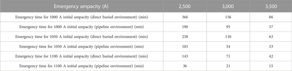
TABLE 5. Comparison of the emergency time for the submarine cable in direct buried environment and pipeline environment.

When the initial ampacity is 1050 A, the working temperatures of the submarine cable core are 346.47 K and 352.88 K respectively in the direct buried environment and the pipeline environment when reaches the thermal equilibrium steady state. When the emergency ampacities of 2500 A, 3000 A and 3500 A are applied, the submarine cable core temperature rises from 346.47 to 363.15 K in 238, 110, and 63 min in the direct buried environment; while in the pipeline environment, the submarine core temperature reaches the maximum allowable temperature after 103, 54, and 33 min.

When the initial ampacity is 1100 A, the working temperatures of the submarine cable core are 350.57 and 355.88 K respectively in the direct buried environment and the pipeline environment when reaches the thermal equilibrium steady state. When the emergency ampacities of 2500 A, 3000 A and 3500 A are applied, the submarine cable core temperature rises to 363.15 K in 143, 71, and 42 min in the direct buried environment; while in the pipeline environment, the submarine core temperature reaches the maximum allowable temperature after 36, 21, and 15 min.

Before applying the emergency ampacity, the submarine core temperature in the direct buried environment is lower than that of the pipeline environment, and hence there is more margin for the submarine core temperature to rise to the maximum allowable temperature. On the other hand, in the landing section of submarine cable, when the environmental factors are the same, the heat dissipation in the pipeline environment is worse than that of the direct buried environment due to the poor thermal conductivity of air in the pipeline. Therefore, when the same emergency ampacity is applied, the submarine core temperature in the pipeline environment will reach the limit value faster.

4 Conclusion

A multi-physical field coupling simulation model by FEM for the landing section of 500 kV AC XLPE EHV submarine cable is established, which is also verified by the TCM. The overload capacity in two typical layout environments is analyzed. The results show that.

(1) When the submarine cable is in direct buried environment, the temperature of B1 phase cable core is the highest, which is 3.86°C higher than that of phase A and phase C cable core. When the submarine cable is in pipeline environment, the temperature of B2 phase cable core is the highest, which is 5.4°C higher than that of phase A and phase C cable core.

(2) When the emergency ampacity is the same, the emergency time decreases with the initial ampacity increased. When the submarine cable is in direct buried environment, the allowed emergency time with the initial ampacity of 1000 A is about 2 times of that with the initial ampacity of 1100 A. When the submarine cable is in pipeline environment, the allowed emergency time with the initial ampacity of 1000 A is about 4 times of that with the initial ampacity of 1100 A.

(3) When the initial ampacity is the same, the emergency time decreases with the emergency ampacity increased. When the emergency ampacity is 2500 A, the allowed emergency time is the longest. When the emergency ampacity is 3500 A, the allowed emergency time is the shortest. The allowed emergency time with the emergency ampacity of 2500 A is about 4 times that with the emergency ampacity of 3500 A.

(4) When the initial ampacity and emergency ampacity are the same, the maximum allowable emergency time in direct buried environment is about 2–3 times of that in pipeline environment.

The results show that the 500 kV AC XLPE submarine cable has a certain overload capacity and can withstand a certain emergency ampacity in a short period. The proposed model can provide a reference for dynamic capacity control of the extra high voltage submarine cable.

Data availability statement

The original contributions presented in the study are included in the article/supplementary material, further inquiries can be directed to the corresponding author.

Author contributions

All authors listed have made a substantial, direct, and intellectual contribution to the work and approved it for publication.

Funding

This work was supported by the Science and Technology Project of State Grid Corporation of China (Grant No. 52060021006H).

Conflict of interest

Authors HZ, GM and PL were employed by State Grid Shandong Electric Power Research Institute. Author YH was employed by 2State Grid Fujian Electric Power Research Institute. The remaining authors declare that the research was conducted in the absence of any commercial or financial relationships that could be construed as a potential conflict of interest.

The authors declare that this study received funding from State Grid Corporation of China. The funder had the following involvement in the study: data collection and analysis.

Publisher’s note

All claims expressed in this article are solely those of the authors and do not necessarily represent those of their affiliated organizations, or those of the publisher, the editors and the reviewers. Any product that may be evaluated in this article, or claim that may be made by its manufacturer, is not guaranteed or endorsed by the publisher.

References

Bian, J., Li, Y., and Shan, L. (2019). Analysis of steady-state heat path model and calculation of current carrying capacity for 500 kV power cable[J]. J. Insulation Mater. 52 (9), 96–101. doi:10.16790/j.cnki.1009-9239.im.2019.09.017

CrossRef Full Text | Google Scholar

Cable design standard for power engineering: GB 50217-2018[S]. Beijing: China Planning Press, 2018.

Google Scholar

Chen, Y., Li, H., and Yao, K. (2021). Analysis on overload capacity of 500kV oil-filled submarine cable[J]. Adv. Technol. Electr. Eng. Energy 40 (10), 1–9. doi:10.12067/ATEEE2104001

CrossRef Full Text | Google Scholar

Duan, J., Yin, C., and Lv, A. (2014). Analysis method for temperature of high voltage submarine cable based on IEC60287 and finite element[J]. High. Volt. Appar. 50 (1), 1–6.

Google Scholar

Duraisamy, N., Gooi, H. B., and Ukil, A. (2018). “Ampacity estimation for HV submarine power cables installed in saturated seabed,” in IEEE international conference on power electronics, Chennai, India (IEEE).

CrossRef Full Text | Google Scholar

Guo, Y., Wei, X., and Yu, Q. (2020). Electrical parameters calculation of 220 kV optical fiber composited three-core submarine cable[J]. Shandong Electr. Power 47 (11), 28–33. doi:10.3969/j.issn.1007-9904.2020.11.006

CrossRef Full Text | Google Scholar

Hao, Y., Chen, Y., and Yang, L. (2017). Coupled simulation on electro-thermal-fluid multiple physical fields of HVDC submarine cable[J]. High. Volt. Eng. 43 (11), 3534–3542. doi:10.13336/j.1003-6520.hve.20171031007

CrossRef Full Text | Google Scholar

Hu, L., Ouyang, B., and Liu, Z. (2019). Improvement in current carrying capacity of landing section of AC 500 kV submarine cable [J]. High. Volt. Eng. 45 (11), 3421–3428. doi:10.13336/j.1003-6520.hve.20191031003

CrossRef Full Text | Google Scholar

IEC 60287-1-1 (1994). Calculation of the current rating of electric cables, part1: Current rating equations (100% load factor) and calculation of losses. IEC 60287-1-1.

Google Scholar

IEC 60287-1-2 (1994). Calculation of current rating of electric cables, part1: Current rating equations (100% load factor) and calculation of losses, section 2: Sheath eddy current loss factor for two circuits in flat formation. IEC 60287-1-2.

Google Scholar

Lei, C., Liu, G., and Ruan, B. (2012). Experimental research of dynamic capacity based on conductor temperature-rise characteristic of HV single-core cable[J]. High. Volt. Eng. 38 (6), 1397–1402. doi:10.3969/j.issn.1003-6520.2012.06.017

CrossRef Full Text | Google Scholar

Liang, Y., Li, Y., and Chai, J. (2007). A new method to calculate the steady-state temperature field and ampacity of underground cable system[J]. Trans. China Electro Tech. Soc. 22 (8), 185–190. doi:10.3321/j.issn:1000-6753.2007.08.034

CrossRef Full Text | Google Scholar

Liang, Z., Xu, M., and Chen, F. (2019). Thermal characteristics of EHV submarine cable in typical layout environments[J]. High. Volt. Eng. 45 (11), 3452–3458. doi:10.13336/j.1003-6520.hve.20191031007

CrossRef Full Text | Google Scholar

Lin, X., He, X., Chen, G., and Xu, C. (2018). RNA-binding protein LIN28B inhibits apoptosis through regulation of the AKT2/FOXO3A/BIM axis in ovarian cancer cells. Study Opt. Commun. 205 (1), 23–26. doi:10.1038/s41392-018-0026-5

CrossRef Full Text | Google Scholar

Lin, Y., Hu, Y., Li, Q., and Cingolani, E. (2021). Pathogenesis of arrhythmogenic cardiomyopathy: Role of inflammation. J. Electron. Meas. Instrum. 35 (11), 39–46. doi:10.1007/s00395-021-00877-5

CrossRef Full Text | Google Scholar

Liu, W. (2020). Research on the carrying capacity of 500 kV high voltage cable in tunnel[D]. Guangzhou: South China University of Technology.

Google Scholar

Liu, Y., Zhang, S., and Cao, J. (2020). Simulation on thermal and electric field of 500 kV HVDC XLPE submarine cable[J]. High. Volt. Appar. 56 (12), 7–15. doi:10.13296/j.1001-1609.hva.2020.12.002

CrossRef Full Text | Google Scholar

Lu, Y., Fan, M., Zheng, M., Scott, M. P., and Evans, M. M. S. (2020). Insights into the molecular control of cross-incompatibility in Zea mays. Guangdong Electr. Power 33 (5), 117–128. doi:10.1007/s00497-020-00394-w

CrossRef Full Text | Google Scholar

Lv, A., Li, Y., and Li, J. (2014). Strain and temperature monitoring of 110 kV optical fiber composite submarine power cable based on brillouin optical time domain reflectometer[J]. High. Volt. Eng. 40 (2), 533–539. doi:10.13336/j.1003-6520.hve.2014.02.028

CrossRef Full Text | Google Scholar

Niu, H., Guo, S., and Yu, J. (2018). Time-space characteristics of current-carrying capacity bottleneck of complicatedly laid transmission cable line[J]. South. Power 12 (5), 44–50. doi:10.13648/j.cnki.issn1674-0629.2018.05.007

CrossRef Full Text | Google Scholar

Qiu, C. (2013). Calculation of temperature field and ampacity of dual-circuit single core power cable with different laying modes and arrangement modes[D]. Guangzhou: South China University of Technology.

Google Scholar

Wang, Q., Lin, Q., Gong, Y., Sun, Y., Feng, J., Guo, R., et al. (2013). Naturally derived anti-inflammatory compounds from Chinese medicinal plants. Shandong Electr. Power 191 (1), 9–39. doi:10.1016/j.jep.2012.12.013

CrossRef Full Text | Google Scholar

Zhang, L., Xuan, Y., and Yue, Y. (2016b). Ampacity calculation, temperature simulation and thermal cycling experiment for 110 kV submarine cable[J]. High. Volt. Appar. 52 (6), 135–140. doi:10.13296/j.1001-1609.hva.2016.06.022

CrossRef Full Text | Google Scholar

Zhang, W., Xiang, Y., Lu, C., Ou, C., and Deng, Q. (2020). Numerical modeling of particle deposition in the conducting airways of asthmatic children. Ship Electr. Technol. 40 (10), 40–46. doi:10.1016/j.medengphy.2019.10.014

CrossRef Full Text | Google Scholar

Zhang, X., Hu, M., and Deng, H. (2016a). Calculation of temperature distribution and ampacity for irregularly arranged power cables based on electromagnetic-thermal-fluid coupled model[J]. J. Insulation Mater. 49 (7), 44–48. doi:10.16790/j.cnki.1009-9239.im.2016.07.009

CrossRef Full Text | Google Scholar

Zhuang, X., Yu, Z., and Niu, H. (2014). Experimental research of relationship between daily load factor and cyclic ampacity of 10 kV XLPE cable[J]. Electr. Power Autom. Equip. 34 (4), 168–172. doi:10.3969/j.issn.1006-6047.2014.04.028

CrossRef Full Text | Google Scholar