 Isaac Hoppman
 Jun Wang
- Department of Engineering Physics, University of Wisconsin, Madison, WI, United States
Fire is one of the most important hazards that must be considered in advanced nuclear power plant safety assessments. The Nuclear Regulatory Commission (NRC) has developed a large collection of experimental data and associated analyses related to the study of fire safety. In fact, computational fire models are based on quantitative comparisons to those experimental data. During the modeling process, it is important to develop diagnostic health management systems to check the equipment status in fire processes. For example, a fire sensor does not directly provide accurate and complex information that nuclear power plants (NPPs) require. With the assistance of the machine learning method, NPP operators can directly get information on local, ignition, fire material of an NPP fire, instead of temperature, smoke obscuration, gas concentration, and alarm signals. In order to improve the predictive capabilities, this work demonstrates how the deep learning classification method can be used as a diagnostic tool in a specific set of fire experiments. Through a single input from a sensor, the deep learning tool can predict the location and type of fire. This tool also has the capability to provide automatic signals to potential passive fire safety systems. In this work, test data are taken from a specific set of the National Institute of Standards and Technology (NIST) fire experiments in a residential home and analyzed by using the machine learning classification models. The networks chosen for comparison and evaluation are the dense neural networks, convolutional neural networks, long short-term memory networks, and decision trees. The dense neural network and long short-term memory network produce similar levels of accuracy, but the convolutional neural network produces the highest accuracy.
1 Introduction and background
1.1 Fire history of nuclear power plant
The United States (U.S.) National Fire Protection Association (NFPA) publishes a “Fire Protection Standard for the LWR reactors” every year. The first edition was released in 2001. The U.S. Nuclear Regulatory Commission (NRC) changes some of the NFPA fire protection rules to let reactor operators take different fire protection measures. Meanwhile, the NRC treats the NFPA rule as an alternative rule. A key part of the approach to adopt these new requirements is an estimation of fire hazards using mathematical models that estimate the potential fire risk. The whole process includes experimental research, measurement uncertainty analyses, fire modeling developments, and the probabilistic risk assessment (PRA) of fire hazards. This reported work mainly summarizes the development of a diagnostic health management classification model that can decide the type and location of a fire. The details include the deep learning classification model sensitivity analysis and data source sensitivity analysis. The work in this research is expected to help advance reactors’ fire safety.
1.2 Fire experimental data for nuclear power plant fire risk analyses
The U.S. Electric Power Research Institute (EPRI) worked with the NRC to develop a database for real fire cases in U.S. nuclear power plants. It is one of the most important databases for fire risk analysis. At the same time, a global fire cases database was developed by the Organization for Economic Co-operation and Development (OECD) Nuclear Energy Agency (NEA) (Beilmann et al., 2019). The NRC’s report NUREG-2169 provides the assumption of ignition frequency and non-suppression probability by using the EPRI’s database (Power Research Institute, 2015). In a separate report, the EPRI updated its Fire Events Database (FEDB) for the period of 1990–2014 (Baranowsky and Facemire, 2013; Lindeman, 2016). Researchers have used these data to validate fire models to help improve their accuracy and effectiveness. A separate database from the Central Research Institute of Electric Power Industry (CRIEPI) was used to find the fire ignition frequency distribution in fire risk analyses for Japanese NPPs (Nagata et al., 2020). This database was used in conjunction with NUREG-2169 to determine whether more than 70% of fire events was related to electrical cabinets, pumps, and transients.
It is important to understand better the ignition mechanism for most common fire events in an NPP. To facilitate this, many researchers have assessed historical fire records. Keski-Rahkonen and Mangs (2002) established the most common electrical ignition mechanism by studying several different databases. They found that the most common cause of electrical ignition was short circuits, ground shorts, and loose connections that led to overheating from the affected cables. They also studied the databases from 1965 to 1989 to catalog the failed components in these fires. Their work found that wiring, cables, or bus connections contribute to 21% of the overall failed components (Keski-Rahkonen et al., 1999). The OECD corroborates this in their findings that electrical equipment causes most of the in-building fires and the most popular fire load is the cable (Angner et al., 2007). Cables increasingly wear off with time, and the fire risk also increases along with this process. However, U.S. and South Korean tests have shown inconsistent cable wearing off patterns and, consequently, inconsistent fire risks (Lee et al., 2017).
Since most of the data are old and some pieces may be missing, new technologies are required to understand and check these data for quality. To facilitate this, we are developing uncertainty quantification, diagnostics, and classification methods.
1.3 Fire experimental description
The National Institute of Standards and Technology (NIST) had conducted a set of experiments to measure the response times of photoelectric and ionization smoke alarms. These tests were located in a home setting (Bukowski, 2007). The NIST smoke alarm experimental data in this work is selected by the U.S. Nuclear Regulatory Commission, in the report NUREG-1824 supplement 1 and EPRI 3002002182 as the “Verification and Validation of Selected Fire Models for Nuclear Power Plant Applications” (Salley and Lindeman, 2016).
The experiments were conducted in real homes using actual furniture and household items as fire sources. The tests were conducted in two different homes. One was a one-story house, and the other a two-story house. Twenty-seven experiments were carried out in the one-story house and eight experiments were carried out in the two-story house, totaling to thirty-six experiments in all. Five different types of fires were considered, namely, smoldering and ignition of chairs in the living room, smoldering mattresses, ignition of beds in the bedroom, and burning cooking oil in the kitchen.
The drawing of the house is shown in Figures 1, 2. Its maximum height is 2.4 m (7.9 ft). The outer walls are 2.1 m (6.9 ft) tall. The ceiling is sloped to 8.4°. The doors of the bathroom and Bedroom 3 are closed during every experiment.
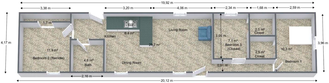
FIGURE 1. Geometry of the experimental facility (Bukowski, 2007).
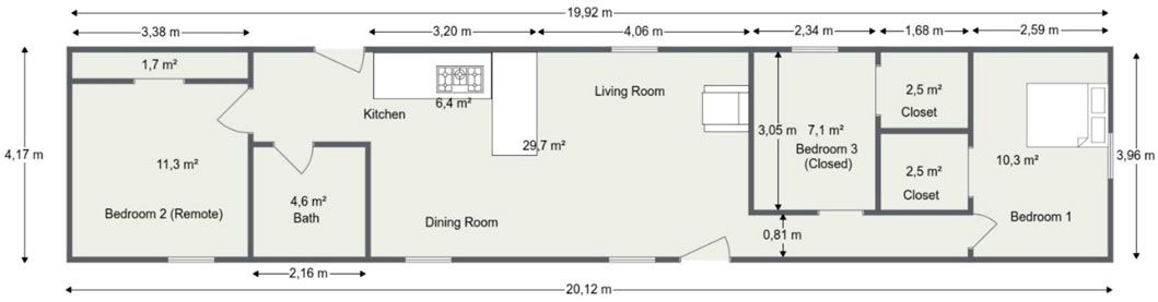
FIGURE 2. Sectional view of the experimental facility (Bukowski, 2007).
The main focus of the experiments was on the smoke alarms. However, other types of alarms were also included. Smoke alarms were placed in the middle of at least one bedroom, in the same room where the fire was started, and located on the ceiling. Along with these, there were temperature sensors, smoke obscuration sensors, and gas concentration sensors.
1.4 Structure of article
The main steps of this work are summarized in Figure 3.
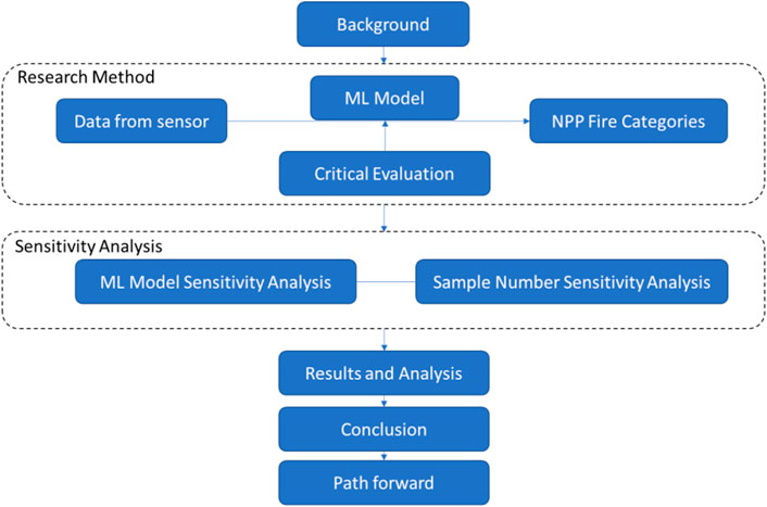
FIGURE 3. Main steps of this work.
2 Research methodology
This study provides a technology to accurately predict the categories (location, ignition, and fire material) of NPP fires depending on the sensor data from temperature sensors, smoke obscuration sensors, gas concentration sensors, and alarms. With the assistance of this technology, operators of nuclear power plants can get more accurate information about NPP fires and take the required actions.
2.1 Classification (output) of this research
In this experiment, we separate the fire location and fire type into five categories, as shown in Table 1.
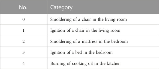
TABLE 1. Category matrix (Bukowski et al., 2003).
The locations in the experiment include the living room, bedroom, and kitchen (Figures 1, 2). The fire types include smoldering, ignition, and burning. With deep learning modeling, we can decide the location and type of fire.
2.2 Fire sensor data (input) types and their data preprocessing technology
Four types of inputs from different sensors were used, which included temperature sensors, smoke obscuration sensors, gas concentration sensors, and alarms (Table 2). The details of each are summarized as follows:
(a) Temperature sensors: in separate rooms, there are seven temperature sensors placed at differing heights from the ceiling. The heights are 20, 300, 610, 900, 1,220, 1,520, and 1,820 mm from the ceiling. These sensors measure the temperature with a thermocouple.
(b) Smoke obscuration sensors: in each room, there are three smoke obscuration sensors placed at varying heights from the ceiling of the rooms. These heights are 20, 610, and 900 mm from the ceiling. These sensors measure the optical density in the room caused by smoke. The data are measured in absorbance units per meter.
(c) Gas concentration sensors: in each room, there are three gas concentration sensors. These sensors measure the concentrations of carbon monoxide, oxygen, and carbon dioxide. They measure the volume of each gas in the air as a percentage of the total volume of the room.
(d) Alarms: inside the alarm sensors, there are two parallel plates that record the voltage between them. The data from the alarms are the voltages from ionization, photoelectric smoke alarms, and CO alarms. When the gasses from the fire come between the plates, they act as a resistor and thus the voltage drops. When this voltage drops low enough, the alarm is set off.
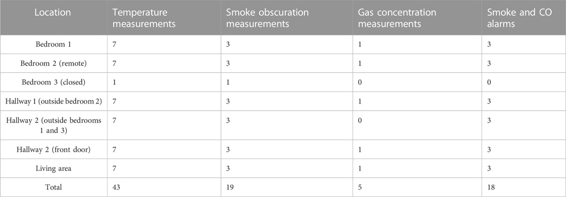
TABLE 2. Number of each sensor type in each location (Bukowski et al., 2003).
There are seven temperature sensors, three smoke obscuration sensors, three gas concentration sensors, and eight types of alarm sensors per room. Since there are six rooms in which there are temperature and smoke obscuration sensors, there are totally 42 temperature sensors and 18 smoke obscuration sensors. Furthermore, there are four rooms that contain gas concentration sensors, that is, there are totally 12 of these sensors. Lastly, there are five rooms that contain alarm sensors, so there are totally 40 alarm sensors. Twenty-five experiments were performed using these same sensors, that is, over the course of the whole database, there are 1,050 temperature time history measurements, 450 smoke obscuration measurements, 300 gas concentration measurements, and 1,000 alarm sensor measurements. All these data are collected in a CSV file, making it very easy to separate the data into its own python arrays to be further utilized.
2.3 Machine learning diagnosis technology, advantages of ML, and models
Different patterns of behavior can be observed for different locations/types of fire accidents. As a result, with a priori knowledge about the specific accident class associated with the measured signal, fire accidents can be identified by the patterns of classification. In this work, four machine learning models, namely, dense neural networks, convolutional neural networks, long short-term memory networks, and decision trees are selected to learn this prior knowledge from the selected database.
Dense neural networks (DNNs) (Figure 4) are a kind of neural network with multiple hidden layers. In theory, the DNN has a stronger data handling capacity with a larger number of hidden layers (Bhardwaj et al., 2018; Bouwmans et al., 2019).
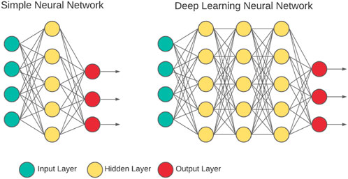
FIGURE 4. Deep learning neural network (Bhardwaj et al., 2018).
Convolutional neural networks (CNNs) (Figure 5) are deep learning networks that are used to solve many types of complex problems, while also overcoming the limitations of traditional machine learning methods. CNNs can efficiently learn the relevant characteristics from many samples and avoid the long and complete process of learning characteristics of the conventional methods (Indolia et al., 2018). The CNN solves problems by imitating how the brain’s visual cortex processes images (Kim, 2017). CNNs are a class of feedforward neural networks that include convolutional computation and have a deep structure and are one of the representative algorithms of deep learning. A typical CNN usually includes four types of layers. These layers are convolution layers, pooling, flattening, and dense layers (Albawi et al., 2017; Bouwmans et al., 2019).
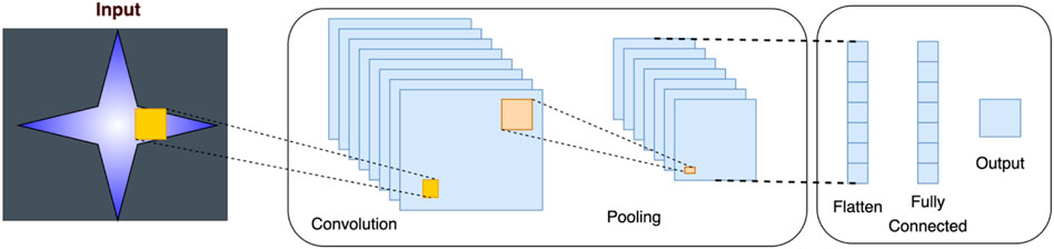
FIGURE 5. Convolutional neural network (Bhardwaj et al., 2018).
Long short-term memory (LSTM) (Figure 6) networks are a kind of optimized recurrent neural network (RNN). The LSTM considers both short-term and long-term dependent relationships (Sherstinsky, 2020; van Houdt et al., 2020). It has a response connection, and can therefore not only model a single data point but also model data sequences. Usually, the LSTM network is made of a cell, an input, an output, and a forget gate. It can deal with the grant extinction problem and is not sensitive to the length of the time gap. Thereby, LSTM networks work well with both short-term and long-term dependent relationships. When constructed, the LSTM model also follows a similar pattern as the CNN model. Instead of repeating convolutional and max-pooling layers, there are repeating LSTM layers followed by flattening and dense layers (Hua et al., 2019).
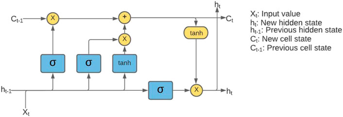
FIGURE 6. Long short-term memory model (Bhardwaj et al., 2018).
Decision trees (DTs) (Figure 7) are a popular data-mining method used to develop the classification system based on multiple variables. This method separates the group into branches like an upside-down tree. These branches include boot notes, internal notes, and leaf notes. This method can deal with large-scale, complete databases without being parameterized (Song and Ying, 2015).
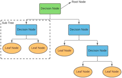
FIGURE 7. Decision tree model (Suthaharan, 2016).
2.4 Accuracy, confusion matrix, precision, recall, and F1 score
There are a few important terms that have to be known to better understand the performance indicators. These terms are true positive, true negative, false positive, and false negative. A true-positive result happens when the true output is correctly predicted as being true.
Accuracy is commonly assessed by the comparison of the prediction and validation results. When simplified, accuracy is basically the ratio of correctly predicted observations to total observations. The classification problem decides the sample classification due to some existing features.
Confusion matrix is a summary of the prediction results in a classification problem (v Stehman, 1997). It summarizes the correct and incorrect results and shows them in a matrix. This is the key to the confusion matrix. The data are arranged into a matrix of outputs. In the example here (Table 1), this is a five-by-five matrix. This indicates that there are five output classes in the model. The data in the columns are the classes predicted by the model. The data in the rows are the actual class of the data (Table 7).
Precision is the ratio of true positives to the total number of true and false positives (Melamed et al., 2003); in other words, the ratio of predicted positives to the total amount of actual positives. Precision is the fraction of how many selected items are relevant. High rates of precision relate to low false-positive rates.
Recall is the ratio of true positives to the total number of true positives and false negatives (Melamed et al., 2003); in other words, the ratio of predicted trues to actual trues. Recall is the percentage of finding relevant cases. Thereby, accuracy and recall are all based on the relevant cases. High rates of recall relate to low rates of false negatives (Figure 8).
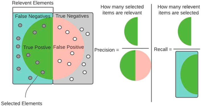
FIGURE 8. Precision and recall (Powers, 2020).
The F score or F measure is a measure of a test’s accuracy. It is based on the calculation’s accuracy or recall. The F score could also be called the harmonic mean (Sasaki, 2007), calculated as follows:
2.5 How to deal with database to make it available for ML model
(a) Select specific data from the database, such as only the temperatures from columns 2–37.
The original databases from the 25 experiments are separated into 25 different CSV files. In each of these files, the data from each type of sensor are ordered sequentially in columns. The temperature sensors are placed first, followed by smoke obscuration, gas concentration, and alarm sensors, in that order. Within these columns, the data are further subdivided into data specifically from sensors in each room. The data from these groups start with data from the remote bedroom, followed by the main bedroom, hallway outside the remote bedroom, hallway outside the main bedroom, living room, and front hallway, in that order.
(b) Gather all the temperature data into a CSV file, then get columns for the 1,050 measurements and rows for the various tables.
Once all the data are in the 25 different CSV files, the required data must be compiled into one singular database. The Pandas and NumPy libraries of python are used to extract the requested data from the CSV files and place them into a list.
(c) Expand and modify the various rows for uniformity.
The machine learning models included in TensorFlow require that all the training data used must be of the same shape and size, that is, every sample must include the same number of data points. Since the data from the original databases are not of the same shape and size throughout all the experiments, some modifications are required. This allows the databases to be effectively reshaped into the required sizes.
3 Case study
Section 3 summarizes the cases that have been studied. The DNN has four layers, the CNN has nine layers, the LSTM network has ten layers, and DTs auto-create the layers. The hyper-parameters of the DNN, CNN, and LSTM network are decided by experience, and a DT is automatically created by itself. There are three groups of data in this work: training, validation, and testing. The validation group is used to avoid over-fitting. We do not set the number of branches in the DT, and it is determined by the machine learning package. For activation, in neural network models (DNN and CNN), this work uses ReLU, and in the LSTM network, tanh is used. The cost function uses cross-entropy for all neural network models (DNN, CNN, and LSTM).
3.1 Sensitivity analysis of machine learning models
This work performed several machine learning model sensitivity analyses and selected the largest sample that we can get from the database and then tested the four selected models. This work reads different data sources, such as temperature data, and then uses the deep learning methods to decide the type and location of the fire. This work compares the experimental results of the categories in Table 1 and summarizes the accuracy results in Table 3.
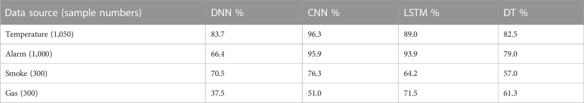
TABLE 3. Prediction accuracy results of the machine leaning model sensitivity analysis.
To make the results easy to compare, we use Figure 9. The y-axis is the percentage of prediction accuracy. As we can see, the convolutional neural network provides the best prediction results. Meanwhile, the predictions based on temperature sensors and alarms are much better, using the advantage of higher sample numbers.

FIGURE 9. Machine leaning model sensitivity analysis.
3.2 Sample number sensitivity analysis
In this section, the research team selects the sample from different numbers of rooms to test the effects of the sample number. First, we assign a letter to each of the rooms. Room A, remote bedroom; room B, main bedroom; room C, hallway outside the remote bedroom; room D, hallway outside the main bedroom; room E, living room; and room F, front door hallway. We list the rooms in each case in Tables 4–6.
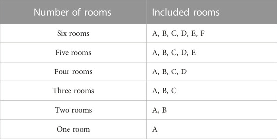
TABLE 4. Rooms included in each case.
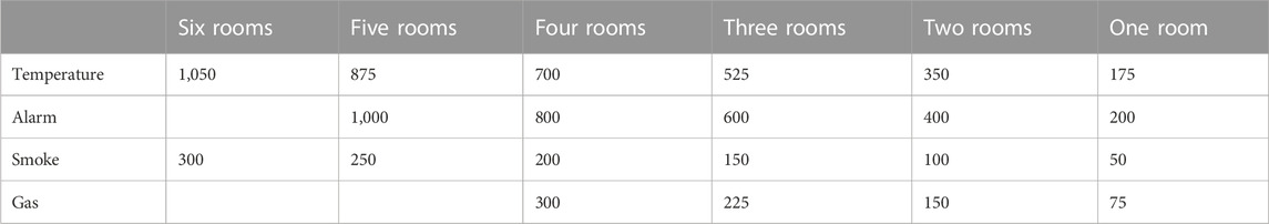
TABLE 5. Sample numbers of each calculation.

TABLE 6. Predicted accuracy of each calculation (%).
To make the results clearer, we also made a figure to show the comparison; the y-axis is the prediction accuracy given in percentage. Figure 10 uses data from Tables 4, 5. As we can see from this figure, evidently, the higher sample number leads to higher prediction accuracy. Meanwhile, the transfer point of the sample number is 500. The temperature data usually provide the best prediction result.
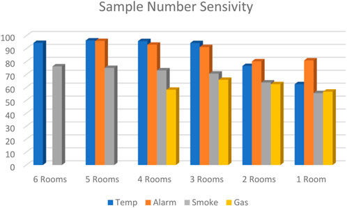
FIGURE 10. Accuracy results of the sensitivity analysis.
3.3 Other results besides the accuracy
The confusion matrix in Table 7 comes from the result of 1,000 temperature sample predictions measured by the conventional neural network. The columns (from left to right) and rows (from top to bottom) are classes 0–4, as described in Table 1. The first column shows that 200 samples belong to class 0 as the experimental data. Meanwhile, the prediction makes some mistakes and some of them are predicted to the other class. This confusion matrix is to explain the mistakes from the deep learning prediction. For example, in the first column, class 0 was predicted correctly as class 0, 195 times. Class 1 was incorrectly predicted as class 0, three times, and class 4 was incorrectly predicted as class 0, two times.

TABLE 7. Confusion matrix.
As we mentioned in the previous sections, we can predict the results of the confusion matrix, accuracy, recall, and F1 score. Due to most of these values being quite similar to the accuracy, we only select the results of the temperature sensor and the 1,050 sample number case as the example to discuss the results. As shown in Table 8, they are quite similar to each other. Thereby, it is reasonable to only use accuracy as the evaluation critical to check the sensitivity analysis result.
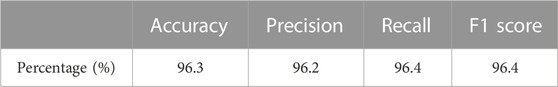
TABLE 8. Precision, recall, and F1-score results.
4 Results and discussion
Four different machine learning models were used on the data to see which model produced the best results. The models used were DNNs, CNNs, LSTM networks, and DTs. These four models were then ranked based on the resultant performance indicators. These indicators were accuracy, confusion matrix, precision, and recall. Accuracy was used as the main indicator. For all four models, the data from the temperature sensors and alarm sensors generally produced the best and most accurate models. There could be a few reasons for this. One reason is that the values for smoke obscuration and gas concentration do not change significantly enough throughout the experiment to accurately predict the type and location of the fire. This may especially be affected by the sensors that are behind closed doors, so smoke and gas exchange between rooms is hindered.
The CNN provided the best overall results. The CNN had the highest accuracy for temperature, alarm, and smoke obscuration data. According to Figure 9, the temperature and alarm data lie in the mid-90s and smoke obscuration in the mid-70s. Within the CNN, the temperature produces the results with the highest accuracy. Accuracy is a good metric to use here because high recall and precision scores show low rates of false positives and false negatives. After the full data set, the data was split into the data received from each of the separate rooms. When the data from at least three of the rooms were taken, the model still produced an accuracy in the mid-90s percentage. Using any fewer rooms than that drops the accuracy to below 75%. For the alarm data, we found the same pattern emerge. This indicates that there was just not enough data to properly train the model when less than three rooms were used.
The next best model was the LSTM model. This is interesting because it is generally regarded to be better at regression than classification. However, LSTM models also work very well with time-based or sequence-based data. Since the data used are organized sequentially with time, this makes it suitable for LSTM models and can thus overcome the deficiencies created when using it for classification. The data type that produced the highest accuracy for this model was the alarm data. Since the model produces better results for data with time dependence, it may be that the alarm data correlates much more strongly with time than does the temperature data. If that is the case, it makes a lot of sense that the alarm data would produce the most accurate results. The LSTM network also follows the same trend as the CNN in the sense that smoke obscuration and gas concentration are still not reliable data types and do not produce good accuracy.
The two data types that produce the lowest accuracy are the DNN and decision tree. Even though they could be strong tools, their capabilities are limited due to the specific conditions in this work. They are ranked equally because overall they produce about the same results. Each model may be better at different data types, but overall they are roughly the same. A DNN is the simplest form of a neural network and the decision tree is one of the simplest forms of tree-based models. Given all this, it is not a surprise that these are the models that produced the lowest accuracies. While each model may produce results that are better than the other, it is mostly meaningless in the sense that neither model produces accuracies high enough to be practically usable (Chen et al., 2018; Chen et al., 2019; Chen et al., 2020a; Chen et al., 2020b; Li et al., 2022).
In Table 8, the CNN shows that all the different classes provide very similar results, with the differences being very minor. For example, the difference between the highest and lowest precision score is 0.2, between the recall scores is 0.3, and between the F1 scores is 0.2. These results help illustrate the fact that the CNN is easily the model that produces the best results.
Another metric that provided highly variable results was the number of rooms the data were taken from. When the data are taken from all the available rooms, the best results are produced, and this is supported by Table 6; when all the rooms were used, the temperature sensor and alarm data were at their highest, in the mid-90s. Smoke obscuration sensors were also at their highest, in the high 70s. The gas concentration is an outlier in this case because it is not at its highest when all rooms are used, but rather it is at its highest when one room is removed. For temperature, alarm, and smoke obscuration sensors, the removal of one room’s worth of data was not too damaging to the accuracy of the model. Temperature and alarm sensors only dropped by about 3% and smoke obscuration only dropped by 4%. The gas concentration was different, as the accuracy increased from the high 50s to the mid60s. The overall temperature sensor data requires the removal of four rooms’ worth of data before the accuracy drops significantly. It dropped from the mid-90s to the mid-70s. The alarm data requires the removal of three rooms for the accuracy to drop from the low 90s to the low 80s. Smoke obscuration sensor data also requires the data of four rooms for the accuracy to drop from the low 70s to the low 60s. In general, it can be said that data from two rooms are not enough to get the maximum accuracy out of the model. However, the jump to three rooms worth of data results in a significant jump in accuracy, getting much closer to the acceptable levels. The main steps of this work have been revised due to these references (Ranjbarzadeh et al., 2021; Anari et al., 2022; Ranjbarzadeh et al., 2022; Saadi et al., 2022; Ranjbarzadeh et al., 2023a; Ranjbarzadeh et al., 2023b).
5 Conclusion
In this work, the authors tried to apply machine learning technology to research fire diagnosis of nuclear power plants. The classification models (DNN, CNN, LSTM network, and DT) were studied and compared to find the model that provides the highest accuracy value. The team also checked differences in accuracy from the models with different amounts of data points. Finally, the team reached the following conclusions:
V.A The conventional neural network (CNN) is the best tool to solve the selected problems.
V.B The sample number in the database can affect the prediction results. The prediction results are better when the number is over 500.
V.C This technology can help to automatically recognize the fire location and type to provide an inlet signal to the potential passive fire protection equipment.
6 Path forward
In the current stage of this work, the accuracy is limited to a maximum of 95%, and it is very hard to improve it further. In addition, not all the necessary data may have been included, and thus a more complete situation is required. The multi-source sensor data fusion provides us with an option to significantly improve the prediction accuracy by completely considering the full inputs from multi-source sensor data. It is not as simple as adding each of the data from multiple sensors. It requires new technology to provide a better analysis method. In the future, the research team will focus on multi-source sensor data to improve the prediction accuracy to a better value. Ultimately, the multi-source data fusion allows us to combine the data from multiple types of sensors to get a complete picture of the events that are happening, rather than just relying on one type of data.
Data availability statement
The original contributions presented in the study are included in the article/Supplementary Material; further inquiries can be directed to the corresponding authors.
Author contributions
IH is the main contributor. IH is the assistant and JW is the mentor.
Funding
This work is supported by the Department of Energy NEUP funding (CFA-20-19671). This work is also supported by the team at Virginia Tech, Prof. Juliana Duarte and Prof. Brian Lattimer.
Conflict of interest
The authors declare that the research was conducted in the absence of any commercial or financial relationships that could be construed as a potential conflict of interest.
Publisher’s note
All claims expressed in this article are solely those of the authors and do not necessarily represent those of their affiliated organizations, or those of the publisher, editors, and reviewers. Any product that may be evaluated in this article, or claim that may be made by its manufacturer, is not guaranteed or endorsed by the publisher.
References
Albawi, S., Mohammed, T. A., and Al-Zawi, S., "Understanding of a convolutional neural network," in 2017 Proceedings of the International Conference on Engineering and Technology, August 21–23, 2017. (Antalya, Turkey: ICET), pp. 1–6.
Anari, S., Sarshar, N. T., Mahjoori, N., Dorosti, S., and Rezaie, A. (2022). Review of deep learning approaches for thyroid cancer diagnosis. Math. Problems Eng. 2022, 1–8. doi:10.1155/2022/5052435
Angner, A., Berg, H. P., Rowekamp, M., Werner, W., and Gauvain, J. (2007). The OECD FIRE project-objectives. Toronto: Status, Applications.
Baranowsky, P., and Facemire, J. (2013). The updated fire events database: Description of content and fire event classification guidance. Palo Alto, CA: Electric Power Research Institute.
Beilmann, M., Bounagui, A., Cayla, J-P., Fourneau, C., Haggstrom, A., Hermann, D., et al. (2019). “Fire safety at nuclear sites: Challenges for the future–an international perspective,” in FSEP 2019 and SMiRT 16th International Post-Conference Seminar on “FIRE SAFETY IN NUCLEAR POWER PLANTS AND INSTALLATIONS, Ottawa, ONT, Canada, October 27-30, 2019.
Bhardwaj, A., Di, W., and Wei, J. (2018). Deep Learning Essentials: Your hands-on guide to the fundamentals of deep learning and neural network modeling. Birmingham, United Kingdom: Packt Publishing Ltd.
Bouwmans, T., Javed, S., Sultana, M., and Jung, S. K. (2019). Deep neural network concepts for background subtraction: A systematic review and comparative evaluation. Neural Netw. 117, 8–66. doi:10.1016/j.neunet.2019.04.024
Bukowski, R. (2007). “Performance of home smoke alarms analysis of the response of several available technologies in residential fire settings (NIST TN 1455-1),” in Technical note (NIST TN) (Gaithersburg, MD: National Institute of Standards and Technology). doi:10.6028/NIST.tn.1455-1r2007
Bukowski, R. W., Peacock, R. D., Averill, J. D., Cleary, T. G., Bryner, N. P., and Reneke, P. A. (2003). Performance of home smoke alarms, analysis of the response of several available technologies in residential fire settings.
Chen, R., Cai, Q., Zhang, P., Li, Y., Guo, K., Tian, W., et al. (2019). Three-dimensional numerical simulation of the HECLA-4 transient MCCI experiment by improved MPS method. Nucl. Eng. Des. 347, 95–107. doi:10.1016/j.nucengdes.2019.03.024
Chen, R., Dong, C., Guo, K., Tian, W., Qiu, S., and Su, G. H. (2020). Current achievements on bubble dynamics analysis using MPS method. Prog. Nucl. Energy 118, 103057. doi:10.1016/j.pnucene.2019.103057
Chen, R., Guo, K., Zhang, Y., Tian, W., Qiu, S., and Su, G. H. (2018). Numerical analysis of the granular flow and heat transfer in the ADS granular spallation target. Nucl. Eng. Des. 330, 59–71. doi:10.1016/j.nucengdes.2018.01.019
Chen, R., Zhang, P., Ma, P., Tan, B., Wang, Z., Zhang, D., et al. (2020). Experimental investigation of steam-air condensation on containment vessel. Ann. Nucl. Energy 136, 107030. doi:10.1016/j.anucene.2019.107030
Powers, D. M. W., "Evaluation: From precision, recall and F-measure to ROC, informedness, markedness and correlation," arXiv preprint arXiv:2010.16061, 2020.
Hua, Y., Zhao, Z., Li, R., Chen, X., Liu, Z., and Zhang, H. (2019). Deep learning with long short-term memory for time series prediction. IEEE Commun. Mag. 57 (6), 114–119. doi:10.1109/mcom.2019.1800155
Indolia, S., Goswami, A. K., Mishra, S. P., and Asopa, P. (2018). Conceptual understanding of convolutional neural network-a deep learning approach. Procedia Comput. Sci. 132, 679–688. doi:10.1016/j.procs.2018.05.069
Keski-Rahkonen, O., and Mangs, J. (2002). Electrical ignition sources in nuclear power plants: Statistical, modelling and experimental studies. Nucl. Eng. Des. 213 (2–3), 209–221. doi:10.1016/s0029-5493(01)00510-6
Keski-Rahkonen, O., Mangs, J., and Turtola, A. (1999). Ignition of and fire spread on cables and electronic components. Tech. Res. Centre Finl. VTT Publ. 387.
Kim, P. (2017). “Convolutional neural network,” in MATLAB deep learning (Berlin, Germany: Springer), 121–147.
Lee, S. K., Moon, Y. S., and Yoo, S. Y. (2017). A study on validation methodology of fire retardant performance for cables in nuclear power plants. J. Korean Soc. Saf. 32 (1), 140–144.
Li, Y., Tian, W., Chen, R., Feng, T., Qiu, S., and Su, G. H. (2022). Research on the nuclear fuel rods melting behaviors by alternative material experiments. J. Nucl. Mater. 559, 153415. doi:10.1016/j.jnucmat.2021.153415
Lindeman, A. (2016). Fire events database update for the period 2010–2014: Revision 1. Palo Alto, Ca: EPRI.
Melamed, I. D., Green, R., and Turian, J. (2003). “Precision and recall of machine translation,” in Companion volume of the proceedings of HLT-NAACL 2003-short papers, 61–63.
Nagata, Y., Uchida, T., and Shirai, K. (2020). The fire event analysis for fire frequency estimation on Japanese nuclear power plant. Int. Conf. Nucl. Eng. 83778, V002T10A004.
Power Research Institute, E. (2015). NUREG-2169 nuclear power plant fire ignition frequency and non-suppression probability estimation using the updated fire events database. Maryland, United States: United States Nuclear Regulatory Commission.
Ranjbarzadeh, R., Caputo, A., Tirkolaee, E. B., Ghoushchi, S. J., and Bendechache, M. (2023). Brain tumor segmentation of mri images: A comprehensive review on the application of artificial intelligence tools. Comput. Biol. Med. 152, 106405. doi:10.1016/j.compbiomed.2022.106405
Ranjbarzadeh, R., Dorosti, S., Ghoushchi, S. J., Caputo, A., Tirkolaee, E. B., Ali, S. S., et al. (2023). Breast tumor localization and segmentation using machine learning techniques: Overview of datasets, findings, and methods. Comput. Biol. Med. 152, 106443. doi:10.1016/j.compbiomed.2022.106443
Ranjbarzadeh, R., Ghoushchi, S. J., Anari, S., Safavi, S., Sarshar, N. T., Tirkolaee, E. B., et al. (2022). “A deep learning approach for robust, multi-oriented, and curved text detection,” in Cognitive computation (Berlin, Germany: Springer).
Ranjbarzadeh, R., Kasgari, A. B., Ghoushchi, S. J., Anari, S., Naseri, M., and Bendechache, M. (2021). Brain tumor segmentation based on deep learning and an attention mechanism using MRI multi-modalities brain images. Sci. Rep. 11, 10930. doi:10.1038/s41598-021-90428-8
Saadi, S. B., Sarshar, N. T., Sadeghi, S., Ranjbarzadeh, R., Forooshani, M. K., and Bendechache, M. (2022). Investigation of effectiveness of shuffled frog-leaping optimizer in training a convolution neural network. J. Healthc. Eng. 2022, 2022.
Salley, M. H., and Lindeman, A. (2016). Nuclear regulatory commission. United States: D.C.Verification and validation of selected fire models for nuclear power plant applications
Sasaki, Y. (2007). The truth of the f-measure. 2007. Available at: https://www.cs.odu.edu/∼mukka/cs795sum11dm/Lecturenotes/Day3/F-measure-YS-26Oct07.pdf (Accessed 05 26, 2021).
Sherstinsky, A. (2020). Fundamentals of recurrent neural network (RNN) and long short-term memory (LSTM) network. Phys. D. Nonlinear Phenom. 404, 132306. doi:10.1016/j.physd.2019.132306
Song, Y.-Y., and Ying, L. U. (2015). Decision tree methods: Applications for classification and prediction. Shanghai archives psychiatry 27 (2), 130–135. doi:10.11919/j.issn.1002-0829.215044
Suthaharan, S. (2016). “Decision tree learning,” in Machine learning models and algorithms for big data classification (Berlin, Germany: Springer), 237–269.
v Stehman, S. (1997). Selecting and interpreting measures of thematic classification accuracy. Remote Sens. Environ. 62 (1), 77–89. doi:10.1016/s0034-4257(97)00083-7
Keywords: fire, nuclear power plants, deep learning, classification, long short-term memory
Citation: Hoppman I, Alhadhrami S and Wang J (2023) Deep learning health management diagnostics applied to the NIST smoke experiments. Front. Energy Res. 11:1175102. doi: 10.3389/fenrg.2023.1175102
Received: 27 February 2023; Accepted: 05 April 2023;
Published: 20 April 2023.
Edited by:
Muhammad Zubair, University of Sharjah, United Arab EmiratesReviewed by:
Ramin Ranjbarzadeh, Dublin City University, IrelandAndaç Batur Çolak, Niğde Ömer Halisdemir University, Türkiye
Copyright © 2023 Hoppman, Alhadhrami and Wang. This is an open-access article distributed under the terms of the Creative Commons Attribution License (CC BY). The use, distribution or reproduction in other forums is permitted, provided the original author(s) and the copyright owner(s) are credited and that the original publication in this journal is cited, in accordance with accepted academic practice. No use, distribution or reproduction is permitted which does not comply with these terms.
*Correspondence: Saeed Alhadhrami, YWxoYWRocmFtaUB3aXNjLmVkdQ==; Jun Wang, anV3YW5nOTgyOTRAb3V0bG9vay5jb20=