POD-based reduced-order modeling study for thermal analysis of gas-cooled microreactor core

Small modular reactors require multi-physics coupling calculations to balance economy and stability, due to their compact structures. Traditional tools used for light water reactors are not effective in addressing the several modeling challenges posed by these calculations. The lumped parameter method is commonly used in the thermal analysis for its high computational speed, but it lacks accuracy due to the thermal model is one-dimensional. While computational fluid dynamics software (CFD) can provide high-precision and high-resolution thermal analysis, its low calculation efficiency making it challenging to be coupled with other programs. Proper Orthogonal Decomposition (POD) is one of the Reduced Order Model (ROM) methods employed in this study to reduce the dimensionality of sample data and to improve the thermal modelling of gas-cooled microreactors. In this work, a non-inclusive POD with neural network method is proposed and verified using a transient heat conduction model for a two-dimensional plate. The method is then applied to build a reduced order model of the gas-cooled micro-reactor core for rapid thermal analysis. The results show that the root mean square error of the reactor core temperature is less than 1.02% and the absolute error is less than 8.2°C while the computational cost is reduced by several orders of magnitude, shortening the calculation time from 1.5-hour to real-time display. These findings proved the feasibility of using POD and neural network in the development of ROMs for gas-cooled microreactor, providing a novel approach for achieving precise thermal calculation with minimized computational costs.

1 Introduction

Advanced small modular reactors (SMRs) have attracted extensive research due to their diverse applications, which were initially motivated by military needs and have been gradually expanded to many civilian fields. Due to their compact structures, SMRs require multi-physics coupling calculations to balance economy and stability during reactor designing, which presents several modeling challenges that cannot be addressed effectively by the traditional tools used for light-water reactors. Taking the integrated design of a gas-cooled microreactor as the example, the lumped-parameter method, which is based on one-dimensional models of physical transport phenomena, is typically used in the thermal-hydraulic analysis. Such a method has high computational efficiency but at the cost of accuracy and resolution. The computational fluid dynamics (CFD) software, on the other hand, is widely used to accurately simulate reactor cores and handle complex geometries, but the enormous computational cost makes it difficult to be coupled with other programs. Therefore, this work focuses on developing a highly accurate thermal model with largely reduced computational cost to serve as a better alternative to the coarse thermal model currently used in integrated simulation.

Reduced-order modeling (ROM) is a powerful modeling technique that can significantly reduce the computational cost while maintaining accuracy. It works by creating a low-dimensional subspace, which is based on the dominant features extracted from the sample data, to approximate the full-state system. This leads to faster calculations from the reduced number of degrees of freedom in the subspace.

An efficient method for creating ROM is the proper orthogonal decomposition (POD)—also known as the Karhunen–Loève expansion, principal component analysis, or empirical orthogonal function (Lorenz, 1956). The POD was first proposed by Pearson (1901) for extracting the main components of big data. Sirovich (1987) used “snapshot” to reduce the dimensionality of the eigenvalue problem, making the POD more efficient and practical for use in various engineering problems, such as in signal analysis, pattern recognition, and fluid dynamics (Liang et al., 2002).

The POD-based ROM can be categorized into two methods: the inclusive and non-inclusive on the basis of whether they require the governing equation of the original system. ROM based on the POD and Galerkin projection is a representative intrusive method which projects the equation onto the subspace basis vector generated by the POD (Hazenberg et al., 2015; Zhang and Xiang, 2015; Gao et al., 2016; Stabile et al., 2017; German and Ragusa, 2019; Star et al., 2019; Sun et al., 2020). By contrast, the non-intrusive ROM is constructed by combining the POD with interpolation methods such as the RBF (Xiao et al., 2015b), Kriging (Chen et al., 2015), and Smolyak (Xiao et al., 2015a). With the rapid development of deep learning, the construction of non-intrusive reduced-order models using neural networks has become a research frontier in recent years. Although the intrusive method offers greater interpretability, its application is limited due to its requirement for accessing the full state equation, as well as instability and non-linear efficiency issues (Amsallem and Farhat, 2012; Washabaugh et al., 2012; Yu et al., 2018). Given the complexity of microreactors, the non-inclusive method based on neural networks is selected to build a reduced-order model in this study. Next is a brief overview of the research status of POD with neural networks.

Wang et al. (2018) applied the POD and long short-term memory (LSTM) to build a reduced-order model for ocean circulation and flow around a cylinder. The results showed that ROM provides high accuracy in numerical prediction, and the CPU time is greatly reduced. Similarly, Ooi et al. (2021) and Wu et al. (2020) used the convolutional neural network to study the flow around a cylinder and compared it with other machine learning methods, such as the regression tree, k-nearest neighbor, etc., which also proved the computational advantages. Unlike the inclusive method, the non-inclusive method can utilize the solution domain as an input parameter as well. For instance, Hasegawa et al. (2020) employed the POD and machine learning to study the unsteady flow around bluff bodies of variable cross sections and proved that these could predict the flow patterns of unknown shapes. To address the challenge of physical constraints in black box models, Swischuk et al. (2019) proposed combining a “particular solution” to modify the results obtained from machine learning to provide a new idea to improve the interpretability of the surrogate model.

In the nuclear industry, the application of ROM based on the POD can be divided into three categories: design and calculation, control optimization, and sensitivity analysis. In the design and calculation field, Sartori et al. (2016) used ROM to perform physical and thermal coupling calculations for a single channel of lead-cooled fast reactor. Star et al. (2021) coupled the RELAP code and ROM to conduct three-dimensional thermal coupling calculations for open and closed pipelines. Kang et al. (2022) used non-inclusive ROM to predict the flow field between reactor rod bundles. In control optimization, Lorenzi et al. (2017) utilized ROM to model the coolant pool of the lead-cooled fast reactor to demonstrate the application of ROM in system-level simulation code. Sensitivity analysis requires many repeated calculations that make it a suitable application for the low-cost calculation capabilities of ROM. For example, Alsayyari et al. (2020) used ROM to perform sensitivity analysis on a simplified molten salt reactor reference model to successfully obtain the relationship between various neutronics and thermal parameters of the system.

In the past three decades, the application of ROM in the nuclear industry has continued to improve with advancements in the model reduction theory and research on the applicability of the POD in heat transfer, Navier–Stokes equation, and neutron transport equations. However, most of the reduced-order models are still at the verification stage to demonstrate their great potential but with limited practical use, especially in the reactor core field. In light of this, this work aims to explore ROM for the gas-cooled microreactor core which balances accuracy and computational efficiency. This new approach could provide valuable insights and serve as the basis for reactor coupling calculations, simulation control, and intelligent operation and maintenance of nuclear power plants.

This article first briefly introduces the research background and previous progress. Section 2 covers the theory of ROM, which includes the calculation of basis and coefficients when using POD and neural network. The following two parts verify and apply ROM using a two-dimensional (2D) plate transient heat conduction problem and thermal analysis of a gas-cooled microreactor. The final part is the conclusion about this work.

2 Method of ROM based on POD

POD aims to find a set of optimal orthogonal basis vectors ${\phi }_1\left(x\right),{\phi }_2\left(x\right),\dots ,{\phi }_k\left(x\right)$ (where ${\phi }_i\left(x\right)$ is a column vector) in the least squares sense, such that the value to be solved of the original system at any time on any node can be expressed as a linear combination of this basis set (Chatterjee, 2000). For instance, considering the node temperature at the domain $x$, the representation is given as

$\mathit{T}\left(\mathit{x},\mathit{t}\right)={\mathit{\alpha }}_{\mathbf{1}}\left(\mathit{t}\right){\mathit{\phi }}_{\mathbf{1}}\left(\mathit{x}\right)+{\mathit{\alpha }}_{\mathbf{2}}\left(\mathit{t}\right){\mathit{\phi }}_{\mathbf{2}}\left(\mathit{x}\right)+\cdots +{\mathit{\alpha }}_{\mathit{k}}\left(\mathit{t}\right){\mathit{\phi }}_{\mathit{k}}\left(\mathit{x}\right),(1)$

where ${\phi }_i\left(x\right)$ is the POD basis and ${\mathrm{\alpha }}_{\mathrm{i}}\left(\mathrm{t}\right),\mathrm{i}=\mathrm{1,2},\cdots ,\mathrm{k}$ are the corresponding coefficients.

In fact, the representation of Eq. 1 is not unique, as the function ${\phi }_i\left(x\right)$ can be represented using different sets of basis functions, such as Legendre polynomials, Chebyshev polynomials, Fourier series, and so on. The sequence of time-functions ${\mathrm{\alpha }}_{\mathrm{i}}\left(\mathrm{t}\right)$ is different for each kind of basis. For the POD, the basis vectors are especially orthogonal, which means this set of basis satisfies

${\mathbf{\phi }}_{{\mathit{k}}_{\mathbf{1}}}\left(\mathit{x}\right)\cdot {\mathbf{\phi }}_{{\mathit{k}}_{\mathbf{2}}}\left(\mathit{x}\right)=\left\{\begin{array}{c}\mathbf{1}\mathrm{i}\mathrm{f}{\mathit{k}}_{\mathbf{1}}={\mathit{k}}_{\mathbf{2}}\\ \mathbf{0}\end{array}\right.,(2)$

${\mathit{a}}_{\mathit{k}}\left(\mathit{t}\right)=\mathit{T}\left(\mathit{x},\mathit{t}\right)\cdot {\mathit{\phi }}_{\mathit{k}}\left(\mathit{x}\right).(3)$

Another characteristic of POD basis is that it consists of a set of ordered column vectors, which makes the approximate accuracy increase as more bases are selected.

Consider a physical field of interest $q$ that is controlled by a mapping function: $\mathrm{q}:\mathcal{X}\times \mathcal{T}\times \mathcal{P}\to \mathbb{R}$, where $\mathcal{X}$ represents the spatial domain, $\mathcal{T}$ represents the time domain, and $\mathcal{P}$ is the input parameter domain. Thus, field $q$ is dependent on the input parameter and varies with time and space conditions. The mapping relationship is generally determined by the physical laws and governing equations, which are often in the form of complicated partial differential equations. These governing equations are discretized into a series of separated points to approximate the solution fields by most traditional numerical solutions that result in large degrees of freedom, especially for three-dimensional and time-varying systems. This leads to high computational requirements. By reducing the dimensionality of the spatial domain, the POD can effectively reduce the computational cost. Next is a brief introduction of the calculation of POD basis ${\phi }_i\left(x\right)$ and coefficients ${\mathrm{\alpha }}_{\mathrm{i}}\left(\mathrm{t}\right)$.

2.1 Calculation of POD basis

The calculation of POD basis relies on a method known as “snapshot,” proposed by Sirovich (1987), which is only dependent on sample data. Consider a distribution $q\left(\cdot ,t; \mathbf{p}\right)$ of field $q$ at time $t\in \mathcal{T}$ and parameter $\mathbf{p}\in \mathcal{P}$. $\mathbf{q}\left(t; \mathbf{p}\right)\in {\mathbb{R}}^{n_x}$, also known as “snapshot,” is a finite dimensional approximation of $q\left(\cdot ,t; \mathbf{p}\right)$ with $n_x$ as the dimension of discretization of the spatial domain. Snapshot is viewed as the true value that can be obtained from experiments or numerical models. A set of snapshots is collected at different times $t_1,\cdots ,t_{n_t}\in \mathcal{T}$ and input parameters ${\mathbf{p}}_1,\cdots ,{\mathbf{p}}_{n_p}\in \mathcal{P}$ to make up a matrix $S\in {\mathbb{R}}^{n_x\times n_s}$, which contains the snapshots as its columns, where $n_s=n_t{n}_p$ (Swischuk et al., 2019). Thus, each row of the matrix represents the value of each discrete point at different times or input parameters, while each column corresponds to the field distribution of all discrete points under the same condition, that is, the snapshot.

According to the theory of POD, the matrix can be written as

$\mathit{S}=\mathit{U}\mathbf{\Sigma }{\mathit{V}}^{\mathbf{T}},(4)$

where

$\mathit{U}{\mathit{U}}^{\mathit{T}}=\mathit{I}\mathit{V}{\mathit{V}}^{\mathit{T}}=\mathit{I}\mathbf{\Sigma }=\mathit{d}\mathit{i}\mathit{a}\mathit{g}\left({\mathit{\sigma }}_{\mathbf{1}},{\mathit{\sigma }}_{\mathbf{2}},\cdots ,{\mathit{\sigma }}_{\mathit{p}}\right),(5)$

with ${\mathrm{\sigma }}_1\ge \mathrm{\sigma }\ge \cdots \ge {\mathrm{\sigma }}_p\ge 0$ and $p=\min \left(n_x,n_s\right)$. $U$ and $V$ are the left and right singular vectors of $S$, respectively, and ${\mathrm{\sigma }}_i$ represents the singular values of $S$. The dimension of $S$ will be reduced by selecting partial columns of $U$ as basis vectors to form a new subspace to approximate $S$. The selection is determined by the value of the corresponding $\mathrm{\sigma }$, which represents the contribution degree of the vector. Since the values of ${\mathrm{\sigma }}_i$ are arranged in the descending order, the first few vectors already contain the main features of the sample data. For example, by extracting the first $k$ columns of $U$ and the first rows of $V$, and retaining the corresponding $\sigma$, we can obtain an optimal approximation of $S$ in the sense of square error, which is expressed as

$\mathit{S}\approx {\mathit{S}}_{\mathit{k}}={\mathit{U}}_{\mathit{k}}{\left(\mathbf{\Sigma }{\mathit{V}}^{\mathbf{T}}\right)}_{\mathit{k}}(6)$

where $U_k=\left({\mathrm{\phi }}_1,{\mathrm{\phi }}_2,\cdots ,{\mathrm{\phi }}_k\right)\in R^{n_x\times \mathrm{k}}$, which is called the POD basis. A typical approach (Holmes et al., 2012; JinXiu et al., 1998) to determine $k$ is

$\frac{{\displaystyle \sum _{\mathit{i}=\mathbf{1}}^{\mathit{k}}}{\mathit{\sigma }}_{\mathit{i}}}{{\displaystyle \sum _{\mathit{j}=\mathbf{1}}^{\mathit{r}}}{\mathit{\sigma }}_{\mathit{j}}}>\mathbf{99.9}\%,(7)$

where $r$ is the rank of matrix $S$. The value is also called energy of the eigenvalue. Eq. 6 can also be written as

$\mathit{A}={\left(\mathbf{\Sigma }{\mathit{V}}^{\mathbf{T}}\right)}_{\mathit{k}}={\mathit{U}}_{\mathit{k}}^{\mathbf{T}}\mathit{S}.(8)$

Matrix $A\in {\mathbb{R}}^{\mathrm{k}\times \mathrm{n}}$ is the projection coefficient of the sample data on the POD basis, then the original problem is transferred from solving $q\left(x,t,p\right)$ to $A\left(t,p\right)$. Since $U_k$ is known, one can obtain the discretization results of $S$ at the spatial domain if $A$ with different times and input parameters is computed. The dimensionality or degree of freedom of $A\left(t,\mathit{p}\right)$ is $k$, which is much smaller than that of $q\left(x,t,\mathit{p}\right)$ (which is $n_x$), making it possible to realize rapid computation.

When the input conditions remain invariant, the field $\left\{\mathbf{q}\left(t_i\right)|i=1,\dots ,n_t\right\}$ becomes a typical transient problem, which is only dependent on time. $U_k$ represents the spatial mode of the sample while $A$ contains time variations. The original system can be predicted by extrapolating the column vector of $A$. On the contrary, the problem becomes stable if the time variable remains invariant, which allows for quick calculation of results for different inputs.

2.2 Calculation of POD coefficients

The non-inclusive method is used to establish a surrogate model that maps input parameters, such as time, pressure, or power, to the coefficients of the POD basis through fitting, interpolation, or other methods, to avoid the need to access and discretize of the governing equation. In fact, Eq. 8 is used to project $S$ onto the basis $U_k$, which gives a set of coefficients for the sample conditions. Thus, a map from the input to coefficients already exists. The coefficients for different parameters can be obtained by fitting this relationship, which is the main idea behind all kinds of non-inclusive methods, such as neural networks.

The artificial neural network, also called neural network in short, is a mathematical model in machine learning that imitates the structure of biological neural networks and can be used for function approximation or estimation. Neurons, which are the computing nodes in a neural network, are interconnected to form a network structure that enables non-linear, parallel, or local computation. A typical neural network comprises three parts:

1 Architecture. It refers to the variables and their topological relationships, which include excitation values and weights of neurons. Figure 1 shows a typical architecture of a neural network.

2 Activation rule. It refers to the functional relationship between the input and output of hidden and output layer nodes, which provides the non-linear ability of the neural network.

3 Learning rules. The learning process involves changing the topological relationship and weight values to reduce the output error within an acceptable range. The rule for modifying the variables is called the learning rule or learning algorithm. The error back propagation (BP) algorithm proposed by Rumelhart et al. (1986) has had the most extensive influence on learning rules and is also used in this work.

FIGURE 1

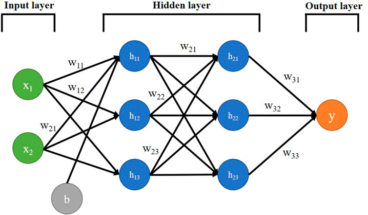
FIGURE 1. Neural network architecture.

The architecture depicted in Figure 1 represents a fully connected feedforward neural network, where every node in each of the layers of the network is connected to all the nodes in the next layer (for simplicity, bias $b$ is only connected to the first neuron of the first hidden layer). Information is transmitted from left to right in a feedforward network, with the input of each layer being the output of the previous layer. The green nodes make up the input layer, where the number of nodes equals the number of input parameters in the sample and is referred to as the input vector. The blue nodes represent the hidden layers, whose number of layers and nodes varies depending on the specific problem and is related to the non-linearity of the neural network. Typically, the number of hidden nodes is greater than the number of input nodes, such as 1.2 to 1.5 times the number of input nodes. Finally, the orange nodes form the output layer, where the number of nodes equals the number of output parameters in the model and is referred to as the output vector.

The data set is typically divided into three parts: the training set, validation set, and test set. The training set is used to train the algorithm, while the validation set is used to calculate the network’s accuracy or error in order to optimize the model parameters. The final model is then evaluated on the test set to measure its error under real conditions.

In this work, a simple neural network and the long short-term memory (LSTM) network architecture are used to model stable and transient fields, respectively. The LSTM is a type of recurrent neural network that is specifically designed to prevent the output of the network for a given input from either decaying or exploding as it cycles through feedback loops (Yu et al., 2019). This architecture is applicable to a number of sequence learning problems, such as language modeling and translation, speech recognition, and timing problems. The underlying algorithms for these types of neural networks have not been reiterated in this study for they have already been developed in many open-source frameworks.

In summary, the calculation process consists of the following steps:

1 Collecting sample data through observations, numerical models, or other methods to form a snapshot matrix $S$

2 Performing POD on $S$ using Eq. 4

3 Extracting the POD basis using principal Eq. 7

4 Calculating the coefficients using Eq. 8 to create a data set with input condition

5 Constructing a neural network model to learn from the data set and

6 Predicting results for different input conditions using Eq. 6.

The reduced order model is validated and analyzed by measuring its accuracy through deviation from the sample data and comparing its computational efficiency with the acquisition time of the sample data. Two methods are adopted in this work to measure the accuracy, one of which is the root-mean-square error (RMSE) of each snapshot, denoted as

$\mathbf{RMSE}\left(\mathit{n}\right)=\frac{\sqrt{\frac{\mathbf{1}}{{\mathit{n}}_{\mathit{x}}}{\displaystyle \sum _{\mathit{m}=\mathbf{1}}^{{\mathit{n}}_{\mathit{x}}}}{\left({\mathbf{q}}_{\mathit{m}}^{\mathit{R}\mathit{O}\mathit{M}}-{\mathbf{q}}_{\mathit{m}}\right)}^{\mathbf{2}}}}{\mathbf{max}\left(\mathbf{q}\right)-\mathbf{min}\left(\mathbf{q}\right)},\mathit{n}=\mathbf{1,2},\dots ,\mathit{N}.(9)$

Here, $q^{\mathrm{R}\mathrm{O}\mathrm{M}}$ is the result of ROM, $q$ is the true value of snapshot, and $n_x$ is the node number. $N$ is the number of snapshots extrapolated using ROM. The maximum and average of all predicted snapshot errors are compared in the following sections. The other criterion is the absolute error between ROM and the true value.

In terms of calculation cost, a speed ratio is defined in this work, which is represented as

$\mathit{r}=\frac{\mathit{t}}{{\mathit{t}}_{\mathit{R}\mathit{O}\mathit{M}}},(10)$

where $t$ refers to the computational time required for obtaining the true value and $t_{ROM}$ is the corresponding time for obtaining results using ROM. It should be noted that the time required for collecting the sample data and training the model is not considered in $t_{ROM}$, which means $t_{ROM}$ refers to the test time.

3 Verification for 2D transient heat conduction

The method described in Section 2 is validated using a typical 2D plate transient heat conduction problem. As shown in Figure 2, the plate has a length of 0.3 m and a width of 0.2 m and is made of a material with density $\mathrm{\rho }=1000\mathrm{k}\mathrm{g}/{\mathrm{m}}^3$, and the specific heat $c=1000\mathrm{J}/\left(\mathrm{k}\mathrm{g}\cdot \mathrm{K}\right)$ and thermal conductivity $k_x=k_y=100\mathrm{W}/\left(\mathrm{m}\cdot \mathrm{K}\right)$. The initial temperature of the plate is 300 K where its left boundary is adiabatic, bottom boundary has a heat flux of $q=1500\mathrm{W}/{\mathrm{m}}^2$, and right boundary has convection with a heat transfer coefficient $h=50\mathrm{W}/\left({\mathrm{m}}^2\cdot \mathrm{K}\right)$ and bulk temperature $T_f=20$°C. To verify the effectiveness of this method under different transient conditions, different top boundary conditions are employed in Case1 and Case2.

FIGURE 2

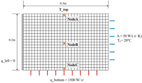
FIGURE 2. 2D plate geometric diagram.

The finite volume method (FVM) is used to obtain the numerical solution, which is regarded as the true value. The mesh model is illustrated in Figure 2, with 30 grids in length and 20 grids in width, resulting in a model with 600 grids and 704 nodes. While the additional source method is used to deal with the boundary conditions, reducing the number of nodes to 600 finally. The time step is 10 s. Nodes A, B, and C are three specific locations selected for comparison with the FVM.

3.1 Case 1: time-varying boundary

In case 1, the upper edge temperature is the time-varying boundary condition with the representation as

$\mathit{T}\_\mathbf{t}\mathbf{o}\mathbf{p}=\mathbf{400}\left(\mathbf{1}-\mathbf{0.5}\mathit{sin}\frac{\mathit{\pi }}{\mathbf{240}}\mathit{t}\right).(11)$

A total of 400 snapshots are obtained by the finite volume model with $t=\mathrm{10,20},\cdots ,4000$ to generate sufficient sample data and constitute the snapshot matrix $S$. The matrix $S$ is decomposed by Eq. 4, and the first four vectors are selected as the POD basis since they account for 99.9% of the energy, as listed in Table 1.

TABLE 1

TABLE 1. Energy ratio of first k eigenvalues of case 1.

The coefficients $\mathrm{\alpha }\left(t\right)\in {\mathbb{R}}^{400\times 4}$ are obtained by projecting the snapshot matrix onto the POD basis, which is used as the training data set for the neural network model. In this work, the LSTM is selected to combine with POD and build the ROM, as it can fit or predict models using historical data, which is especially applicable to time-related variables. The architecture of the proposed POD-LSTM model is shown in Figure 3, which is implemented using Python and Keras. The input of the model are coefficients from the previous four steps and the output is the coefficient at time $t$. The term “DENSE” represents the fully connected layers. Therefore, the relation between the input and the output can be represented as

$\mathit{\alpha }\left(\mathit{t}\right)=\mathit{f}\left(\mathit{\alpha }\left(\mathit{t}-\mathbf{1}\right),\mathit{\alpha }\left(\mathit{t}-\mathbf{2}\right),\mathit{\alpha }\left(\mathit{t}-\mathbf{3}\right),\mathit{\alpha }\left(\mathit{t}-\mathbf{4}\right)\right),(12)$

where $f\left(\cdot \right)$ is a mapping function.

FIGURE 3

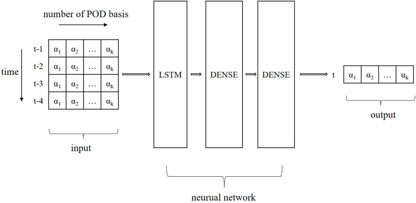
FIGURE 3. LSTM architecture for 2D plate heat conduction.

In this case, the first 60% of the data (0 s–2,400 s) is selected as the training set and the last 40% (2,400 s–4,000 s) as the test set, and then 20% of the data in the training set is divided to be the verification data. The shape of the input vector is (4,4) and the number of nodes in the three hidden layers are 64, 32, and 4, with activation functions of Tanh, Tanh, and Linear, respectively. A batch size of 16 and 50 epochs is used, with the mean square error serving as the loss function, ADAM as the optimizer, and a learning rate of 0.0005 during training.

The temperature distribution of the plate at t = 4,000 s calculated by the reduced-order model as shown in Figure 4A. The temperatures of nodes A, B, and C are shown in Figure 4B to compare the errors, which vary with time. The maximum RMSE is 0.73% and the maximum absolute error is 1.82°C, which indicates that the results obtained from the reduced-order model are in good agreement with those from the finite volume model. As for the computational speed, the FVM model consumes 83.98 s while the training time of the reduced-order model is 9.63 s and the prediction time is 0.02 s, resulting in the speed ratio of $r=4199$. It should be admitted that collecting the sample data is time-consuming and equivalent to the time required for the FVM model. However, once the reduced-order model is established, it can significantly reduce the computational cost.

FIGURE 4

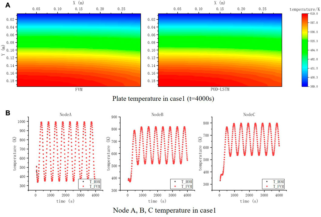
FIGURE 4. Temperature comparison in case 1. (A) Plate temperature in case 1 (t = 4,000 s). (B) Node A, B, and C temperature in case 1.

3.2 Case 2: multiple time-varying boundary

The upper boundary temperature in case 2 comprises nine different time-varying conditions, which can be expressed as

$\mathit{T}\_\mathbf{t}\mathbf{o}\mathbf{p}=\mathit{M}\left(\mathbf{1}-\mathbf{0.5}\mathit{sin}\frac{\mathit{\pi }}{\mathbf{240}}\mathit{t}\right),(13)$

with $M=200,300,\dots ,\mathrm{1,000}$. The snapshot mentioned in Section 2.1 is only related to time, while the temperature in this case has two parameters: time $t$ and amplitude $M$. Thus, the snapshot matrix is a combination of all sub-matrixes at the same $M$ in the row vector direction, which is shown in Eq. 14. Subscript $p$ represents different parameters, that is, different $M$ in case 2. Then, the POD basis can be obtained using Eq. 4 as in the previous case.

${\mathit{S}}_{{\mathit{p}}_{\mathbf{1}}}=\left(\begin{array}{ccc}{\mathit{T}}_{\mathbf{11}}\left({\mathit{t}}_{\mathbf{1}},{\mathit{p}}_{\mathbf{1}}\right)& \cdots & {\mathit{T}}_{\mathbf{11}}\left({\mathit{t}}_{\mathit{n}},{\mathit{p}}_{\mathbf{1}}\right)\\ ⋮& \ddots & ⋮\\ {\mathit{T}}_{\mathit{M}\mathit{N}}\left({\mathit{t}}_{\mathbf{1}},{\mathit{p}}_{\mathbf{1}}\right)& \cdots & {\mathit{T}}_{\mathit{M}\mathit{N}}\left({\mathit{t}}_{\mathit{n}},{\mathit{p}}_{\mathbf{1}}\right)\end{array}\right),$

$\mathit{S}=\left(\begin{array}{ccc}{\mathit{S}}_{{\mathit{p}}_{\mathbf{1}}}& \cdots & {\mathit{S}}_{{\mathit{p}}_{\mathrm{J}}}\end{array}\right)=\left(\begin{array}{ccc}{\mathit{T}}_{\mathbf{11}}\left({\mathit{t}}_{\mathbf{1}},{\mathit{p}}_{\mathbf{1}}\right)& \cdots & {\mathit{T}}_{\mathbf{11}}\left({\mathit{t}}_{\mathit{n}},{\mathit{p}}_{\mathit{J}}\right)\\ ⋮& \ddots & ⋮\\ {\mathit{T}}_{\mathit{M}\mathit{N}}\left({\mathit{t}}_{\mathbf{1}},{\mathit{p}}_{\mathbf{1}}\right)& \cdots & {\mathit{T}}_{\mathit{M}\mathit{N}}\left({\mathit{t}}_{\mathit{n}},{\mathit{p}}_{\mathit{J}}\right)\end{array}\right).(14)$

Unlike Eq. 12, the coefficients in case 2 include the influence of parameter $M$, thus the fitting relationship becomes

$\mathit{\alpha }\left(\mathit{t}\right)=\mathit{f}\left(\mathit{\alpha }\left(\mathit{t}-\mathbf{1}\right),\mathit{M},\mathit{t}\right),(15)$

where $f\left(\cdot \right)$ is a mapping function.

The sample data consist of 1,800 snapshots with $t=10,20,\cdots ,\mathrm{2,000}$ and $M=200,300,\dots ,\mathrm{1,000}$. The first five bases are retained for they meet principal Eq. 7 as shown in Table 2.

TABLE 2

TABLE 2. Energy ratio of first k eigenvalues of case 2.

In total, 80% of the data set is used for training, and the remaining 20% is the validation set. The test data is the temperature when M = 350 and 1,100, which are not included in the snapshot matrix. The shape of the input vector is (1,7) and the number of nodes in the three hidden layers are 100, 32, and 5 with activation functions of Tanh, Tanh, and Linear, respectively. The batch size is 8 and epoch is 100, loss function is the mean square error, optimizer is ADAM, and learning rate is 0.001. The temperature of the plate at t = 0–2,000 s is calculated using ROM and compared with the FVM results.

The temperature comparison is as shown in Figures 5A, B. The maximum RMSE is 5.63% and maximum absolute error is 4.07°C when M = 350, and the maximum RMSE is 5.50% and maximum absolute error is 12.72°C when M = 1,100. The accuracy of the temperature for M = 1,100 is slightly worse than that for M = 350, which indicates that the ability of extrapolation is not very satisfactory, as for all predictions are based on the known sample data. The computational cost comparison is represented in Table 3, which shows ROM can achieve fast calculations.

FIGURE 5

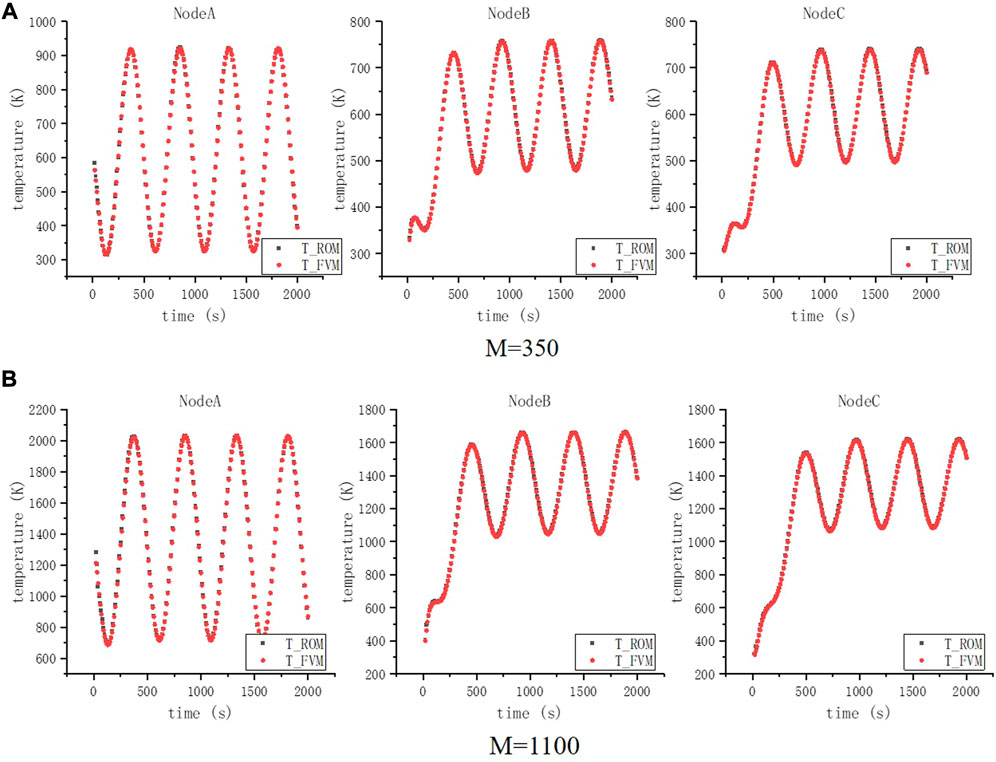
FIGURE 5. Node A, B, and C temperature in case 2. (A) M = 350 and (B) M = 1,100.

TABLE 3

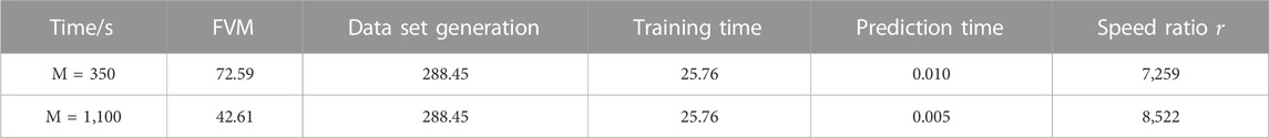
TABLE 3. Computational cost comparison in case 2.

3.3 Analysis

In summary, the reduced-order model has demonstrated excellent accuracy and computational efficiency in case 1, while there is still room for improvement in accuracy for the more complex transient problem in case 2. It is worth noting that the distinction between transient and stable states is not evident, as they merely represent different input parameters for the neural network. Extrapolation remains a significant challenge for this method, as the neural network can only provide reasonable predictions based on known sample data. Despite being appropriate for time-series problems, even the LSTM model has limitations in addressing this challenge, as errors may accumulate gradually over prediction time. It is worth noting that the reduced-order model constructed using the POD and neural network method does not involve any governing equations or physical laws. Instead, it relies on a vast amount of sample data and optimization algorithms. Therefore, using different samples and algorithms to construct a reduced-order model could lead to better results for the two cases. But the acceleration effect of the reduced-order model underscores its potential for efficient predictions, once the model has been optimized to meet the desired accuracy requirements.

4 ROM for gas-cooled microreactor thermal analysis

4.1 CFD model for gas-cooled microreactor core

4.1.1 Layout of reactor core

This work presents the detailed modeling of a horizontal compact high-temperature gas-cooled reactor with a designed thermal power of 5 MWth. The reactor is composed of fuel assembly, control rod assembly, reflector, boron carbon brick, and other components. The core layout and fuel assembly configuration are illustrated in Figures 6A, B, respectively. The active zone of the horizontal core comprises hexagonal fuel assemblies that are organized into four layers in the axial direction, with each containing 60 fuel assemblies. As such, the entire reactor contains 240 fuel assemblies, with varying degrees of enrichment at different positions. The core has a total radial diameter (to the outer edge of the reflector) of 210 cm and a total axial length of 220 cm. The active zone has an equivalent diameter of 131 cm and a length of 164 cm. The core side reflector consists of 12 groups of regulating control rods, while a single group of control rods is located at the center. The coolant is single-phase helium, which is not coupled with reactivity and does not undergo any chemical reactions with the cladding and fuel structural materials. The reflectors are made of graphite, which also acts as the neutron moderator and core structure material.

FIGURE 6

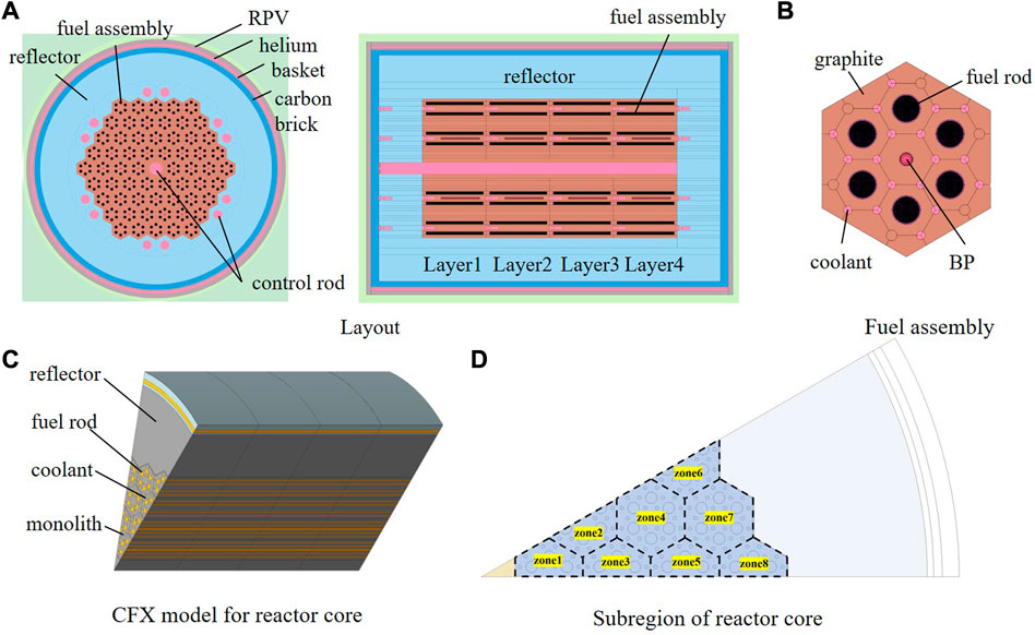
FIGURE 6. Layout and CFX model of reactor core. (A) Layout. (B) Fuel assembly. (C) CFX model for reactor core. (D) Subregion of reactor core.

4.1.2 Thermal analysis with CFX

A three-dimensional thermal modeling of the active zone in the reactor core is conducted using ANSYS CFX 2020. This model includes 1/12 of the entire core to take advantage of the symmetrical characteristic, as depicted in Figure 6C, with a mesh number of 2.77 million. Two significant boundary conditions are considered in this model. The first condition is the power density of fuel rods, denoted as $S_{\mathrm{z}\mathrm{o}\mathrm{n}\mathrm{e}\mathrm{i}}$. The subscript “zone,” shown in Figure 6D, refers to the different parts of the core. As mentioned, each fuel rod consists of four fuel assemblies in the axial direction, and one fuel assembly contains 11 fuel pellets. Therefore, the power distribution of each fuel rod has 44 points, resulting in the expression of power density $S_{\mathrm{z}\mathrm{o}\mathrm{n}\mathrm{e}\mathrm{i}}\in {\mathbb{R}}^{8\times 44}$, that is,

${\mathit{S}}_{\mathbf{zonei}}=\mathbf{1.0014}{\mathit{P}}_{\mathbf{zonei}}\cdot \frac{{\mathit{P}}_{\mathbf{total}}}{\mathbf{60}\times {\mathit{V}}_{\mathbf{zonei}}}\mathit{i}=\mathbf{1,2},\dots ,\mathbf{8},(16)$

where 1.0014 is an empirical factor used in the thermal calculation of the CFX model to ensure energy conservation, $P_{\mathrm{z}\mathrm{o}\mathrm{n}\mathrm{e}\mathrm{i}}\in {\mathbb{R}}^{8\times 44}$ is the normalized power factor of each region, which is calculated by a neutronics model and is dependent on the lifetime of the reactor. $P_{\mathrm{t}\mathrm{o}\mathrm{t}\mathrm{a}\mathrm{l}}=5\mathrm{M}\mathrm{W}$ is the design thermal power, and $V_{\mathrm{z}\mathrm{o}\mathrm{n}\mathrm{e}\mathrm{i}}$ is the volume of fuel rods in each region, which is directly stored in the CFX model. The number 60 represents the division of the core into four layers in the axial direction, with each layer containing 60 fuel assemblies.

The other boundary is the flow of the coolant. The outlet of the reactor is at atmospheric pressure and outlet temperature is 750°C at load tracking operation. Therefore, the flow of the coolant can be represented as

$\mathit{Q}=\frac{\mathbf{1}}{\mathbf{12}}\cdot \frac{{\mathit{P}}_{\mathbf{total}}}{\left({\mathit{T}}_{\mathbf{reactorOutlet}}-{\mathit{T}}_{\mathbf{reactorInlet}}\right){\mathit{C}}_{\mathrm{p}}}\cdot \left(\mathbf{1}-{\mathit{Q}}_{\mathbf{bypass}}\right),(17)$

where $T_{\mathrm{r}\mathrm{e}\mathrm{a}\mathrm{c}\mathrm{t}\mathrm{o}\mathrm{r}\mathrm{O}\mathrm{u}\mathrm{t}\mathrm{l}\mathrm{e}\mathrm{t}}=750$°C, $C_{\mathrm{p}}=5195\mathrm{J}/\left(\mathrm{k}\mathrm{g}\cdot \mathrm{K}\right)$ is the specific heat of helium, $Q_{\mathrm{b}\mathrm{y}\mathrm{p}\mathrm{a}\mathrm{s}\mathrm{s}}=0.12$ is the portion of the bypass flow, and the number 1/12 refers that only 1/12 of the core is considered.

In summary, the state of the core is dependent on the normalized power factor $P_{\mathrm{z}\mathrm{o}\mathrm{n}\mathrm{e}\mathrm{i}}\in {\mathbb{R}}^{8\times 44}$ (which is relies on the lifetime) and temperature of the coolant upon entering the reactor $T_{\mathrm{r}\mathrm{e}\mathrm{a}\mathrm{c}\mathrm{t}\mathrm{o}\mathrm{r}\mathrm{I}\mathrm{n}\mathrm{l}\mathrm{e}\mathrm{t}}$ .For example, considering a lifetime of 1000 EFPD (effective full-power days) and a coolant temperature of 488.7°C, the temperature of the core and monolith is shown in Figure 7. The maximum temperature of the fuel and monolith are 981.2°C and 902.2°C, respectively. It is worth noting that the temperature increases along the flow of the coolant in the axial direction and zone 4 is the hot zone.

FIGURE 7

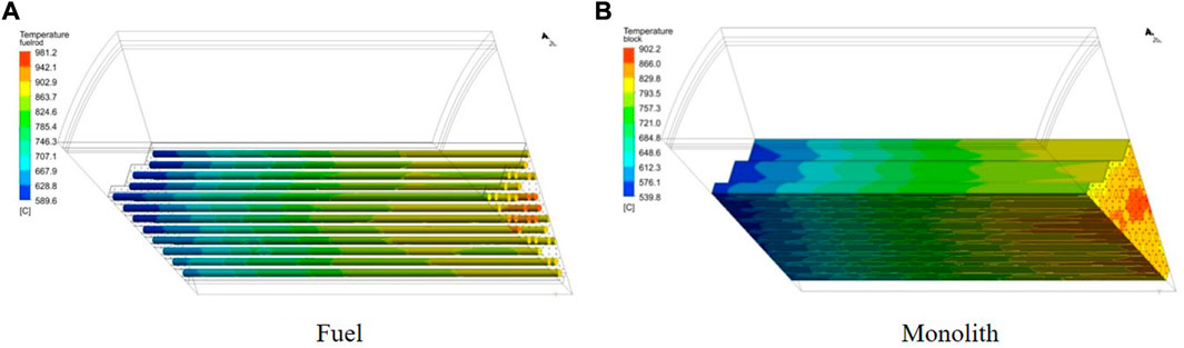
FIGURE 7. Temperature of core (1,000 EFPD, 488.7°C). (A) Fuel. (B) Monolith.

4.2 ROM for thermal analysis of reactor core

4.2.1 Generation of sample data

Zone 4 is selected to build a reduced-order model as this area is a typical region. The first step is to collect sufficient sample data accruing to the abovementioned steps.

4.2.1.1 Power density

There are only seven different power density distributions calculated using the neutronics model due to computational limitations, where $EFPD=0,3.3,250,550,650,750,\mathrm{a}\mathrm{n}\mathrm{d}\mathrm{1,000}$. To generate more input parameters, Hermite interpolation is adopted twice to the power factor, as it is a two-dimensional array. A small random variable is added to each power factor according to certain rules to ensure that the average power factor meets the normalization requirements. Finally, 100 different lifetimes, ranging from 5 EFPD–995 EFPD in iterations of 10 EFPD, are used as input parameters.

4.2.1.2 Temperature of inlet coolant

A trial calculation revealed that the effect of coolant temperature on the results is approximately linear, so it is not necessary to design too many different coolant temperatures. Considering the maximum temperature limit of 550°C for the 316H stainless steel used in the reactor pressure vessel and basket, the range of the coolant inlet temperature is fixed at 200–500°C, with 50°C iteration.

To sum up, in combination with the distribution of power factor and coolant temperature, a total of 700 sets of different input conditions for core temperature are computed, which are taken as the sample data for ROM after format processing. The number of sample data is 36,774 and 19,602 for the fuel rods and monolith, respectively, by extracting nodes coordinates and temperatures in zone 4 (the nodes of the monolith are after selection). The following sections discuss ROM for fuel and monolith, respectively.

4.2.2 ROM for fuel rods zone

Based on the collected sample data, the size of the snapshot matrix is 36,774 × 700 with 700 corresponding eigenvalues, and the first 12 eigenvalues meet the selection principle, accounting for 99.90% of the total. Therefore, the input shape for the neural network is (700,353) and the output shape is (700,12). The training set is composed of 80% of the data, the test set is composed of 20%, and then 20% of data in the training set is divided to be the verification data. The architecture of the model is depicted in Figure 8, with three hidden layers having 64, 32, and 12 nodes, respectively, and activation functions of Tanh, Tanh, and Linear. A batch size of 32 and 150 epochs are used, with the mean square error serving as the loss function, ADAM as the optimizer, with a learning rate of 0.0005 during training.

FIGURE 8

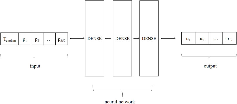
FIGURE 8. Neural network architecture for fuel rods zone.

To verify the accuracy of ROM, the results from six cases are compared with those obtained from the CFX model, as shown in Table 4. Figure 9 presents the temperature contour for the fuel rod in the case with maximum error. The results demonstrate that the average root-mean-square error is 1.02% and maximum absolute error is 8.2°C, indicating a good agreement between the ROM and CFX results. Furthermore, while CFX requires 1.5 h for a single computational core, the test time for the reduced-order model is less than 0.01 s, implying that ROM can achieve real-time display.

TABLE 4

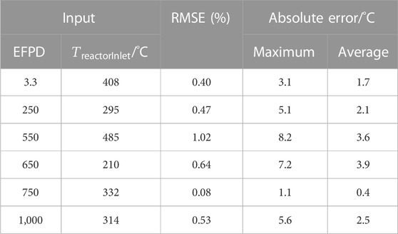
TABLE 4. Comparison between ROM and CFX (fuel rods zone).

FIGURE 9

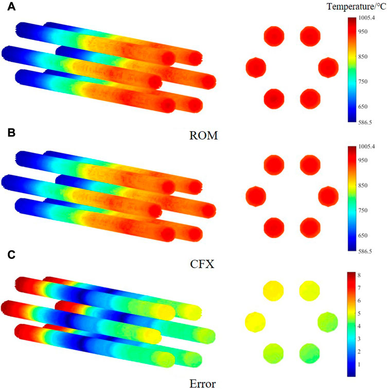
FIGURE 9. Temperature contour comparison for fuel rods zone. (A) ROM. (B) CFX. (C) Error.

4.2.3 ROM for monolith zone

The reduced-order model building process for the monolith zone is similar to that of the fuel rods zone and is therefore not repeated here. But the number of bases for this case is nine. All other parameters are the same as for the previous fuel case, except that the epoch for the monolith model is 200. As shown in Table 5 and Figure 10, the maximum of RMSE is 0.46% and the maximum absolute error is 5.1°C, which also meets the accuracy requirements. The test time in this case is also less than 0.01 s.

TABLE 5

TABLE 5. Comparison between ROM and CFX (monolith zone).

FIGURE 10

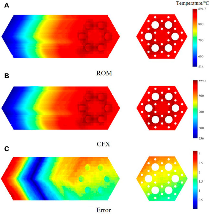
FIGURE 10. Temperature contour comparison for monolith zone. (A) ROM. (B) CFX. (C) Error.

5 Conclusion

This study introduces an approach to ROM that incorporates both POD and neural networks. The method is tested on a 2D transient heat conduction model, and the results demonstrate that ROM is effective in terms of both accuracy and computational speed, especially when dealing with time-varying boundaries. However, for more complex boundaries or problems that requires time-dependent predictions, the error rate increases due to the requirement for a large amount of historical data. Consequently, the model must be updated regularly to ensure accurate predictions. It is worth noting that the reduced-order model created using this approach does not distinguish between the time parameter in transient problems and other variables in steady-state problems. The key concept behind this approach is to reduce data dimensions by capturing the essential features of the sample data to enable fast calculations.

The Section 4 focuses on analyzing the thermal model of a gas-cooled microreactor core using load tracking operation as the reference condition, with future research aiming to consider more complex scenarios such as transient states and accidents. By employing a combination of POD and neural networks, a highly accurate reduced-order model is developed. The results demonstrate that ROM achieves a root-mean-square error of less than 1.02% and an absolute error of less than 8.2°C when predicting core temperature. Furthermore, the computational efficiency of the reduced-order model is greatly improved, reducing the calculation time from 1.5 h to real-time display. These findings provide compelling evidence for the feasibility of using POD and machine learning in the development of reduced-order models for gas-cooled microreactors, offering a novel approach to achieve precise thermal calculation while minimizing computational costs. The research thus holds significant implications for the intelligent operation and maintenance of nuclear power plants, as well as for the many coupled calculations involved in gas-cooled microreactors.

Data availability statement

The original contributions presented in the study are included in the article/Supplementary Material; further inquiries can be directed to the corresponding authors.

Author contributions

EC: methodology, calculation, and writing of the manuscript; HZ: resources and supervision; YY: project administration, resources, and supervision.

Conflict of interest

Authors EC, HZ, and YY were employed by China Nuclear Power Engineering Co., Ltd.

Publisher’s note

All claims expressed in this article are solely those of the authors and do not necessarily represent those of their affiliated organizations, or those of the publisher, editors, and reviewers. Any product that may be evaluated in this article, or claim that may be made by its manufacturer, is not guaranteed or endorsed by the publisher.

References

Alsayyari, F., Tiberga, M., Perkó, Z., Lathouwers, D., and Kloosterman, J. L. (2020). A nonintrusive adaptive reduced order modeling approach for a molten salt reactor system. Ann. Nucl. Energy 141, 107321. doi:10.1016/j.anucene.2020.107321

CrossRef Full Text | Google Scholar

Amsallem, D., and Farhat, C. (2012). Stabilization of projection-based reduced-order models. Int. J. Numer. Methods Eng. 91 (4), 358–377. doi:10.1002/nme.4274

CrossRef Full Text | Google Scholar

Chatterjee, A. (2000). An introduction to the proper orthogonal decomposition. Curr. Sci. Available at: https://www.jstor.org/stable/24103957 78, 808–817.

Google Scholar

Chen, X., Liu, L., and Yue, Z. (2015). Reduced order aerothermodynamic modeling research for hypersonic vehicles based on proper orthogonal decomposition and surrogate method. Acta Aeronaut. Astronaut. Sin. 36 (2), 462–472. doi:10.7527/S1000-6893.2014.0079

CrossRef Full Text | Google Scholar

Gao, X., Hu, J., and Huang, S. (2016). A proper orthogonal decomposition analysis method for multimedia heat conduction problems. J. Heat Transf. 138 (7). doi:10.1115/1.4033081

CrossRef Full Text | Google Scholar

German, P., and Ragusa, J. C. (2019). Reduced-order modeling of parameterized multi-group diffusion k-eigenvalue problems. Ann. Nucl. Energy 134, 144–157. doi:10.1016/j.anucene.2019.05.049

CrossRef Full Text | Google Scholar

Hasegawa, K., Kai, F., Murata, T., and Fukagata, K. (2020). Machine-learning-based reduced-order modeling for unsteady flows around bluff bodies of various shapes. Theor. Comput. Fluid Dyn. 34, 367–383. doi:10.1007/s00162-020-00528-w

CrossRef Full Text | Google Scholar

Hazenberg, M., Astrid, P., and Weiland, S. “Low order modeling and optimal control design of a heated plate,” in Proceedings of the European Control Conference), Cambridge, UK, September 2015. doi:10.23919/ECC.2003.7085130

CrossRef Full Text | Google Scholar

Kang, H., Tian, Z., Chen, G., Li, L., and Wang, T. (2022). Application of POD reduced-order algorithm on data-driven modeling of rod bundle. Nucl. Eng. Technol. 54 (1), 36–48. doi:10.1016/j.net.2021.07.010

CrossRef Full Text | Google Scholar

Liang, Y., Lee, H., Lim, S., Lin, W., Lee, K., and Wu, C. (2002). Proper orthogonal decomposition and its applications—Part I: Theory. J. Sound Vib. 252 (3), 527–544. doi:10.1006/jsvi.2001.4041

CrossRef Full Text | Google Scholar

Lorenz, E. N. (1956). Empirical orthogonal functions and statistical weather prediction. Cambridge, USA: Massachusetts Institute of Technology, Department of Meteorology.

Google Scholar

Lorenzi, S., Cammi, A., Luzzi, L., and Rozza, G. (2017). A reduced order model for investigating the dynamics of the Gen-IV LFR coolant pool. Appl. Math. Model. 46, 263–284. doi:10.1016/j.apm.2017.01.066

CrossRef Full Text | Google Scholar

Ooi, C., Le, Q. T., Dao, M. H., Nguyen, V. B., Nguyen, H. H., and Ba, T. (2021). Modeling transient fluid simulations with proper orthogonal decomposition and machine learning. Int. J. Numer. Methods Fluids 93 (2), 396–410. doi:10.1002/fld.4888

CrossRef Full Text | Google Scholar

Pearson, K. (1901). LIII. On lines and planes of closest fit to systems of points in space. Lond. Edinb. Dublin philosophical Mag. J. Sci. 2 (11), 559–572. doi:10.1080/14786440109462720

CrossRef Full Text | Google Scholar

Rumelhart, D. E., Hinton, G. E., and Williams, R. J. (1986). Learning representations by back-propagating errors. Nature 323, 533–536. doi:10.1038/323533a0

CrossRef Full Text | Google Scholar

Sartori, A., Cammi, A., Luzzi, L., and Rozza, G. (2016). A multi-physics reduced order model for the analysis of Lead Fast Reactor single channel. Ann. Nucl. Energy 87, 198–208. doi:10.1016/j.anucene.2015.09.002

CrossRef Full Text | Google Scholar

Sirovich, L. (1987). Turbulence and the dynamics of coherent structures. I. Coherent structures. Q. Appl. Math. 45 (3), 561–571. doi:10.1090/qam/910462

CrossRef Full Text | Google Scholar

Stabile, G., Hijazi, S., Mola, A., Lorenzi, S., and Rozza, G. (2017). POD-galerkin reduced order methods for CFD using finite volume discretisation: Vortex shedding around a circular cylinder. Commun. Appl. Industrial Math. 8 (1), 210–236. doi:10.1515/caim-2017-0011

CrossRef Full Text | Google Scholar

Star, S. K., Spina, G., Belloni, F., and Degroote, J. (2021). Development of a coupling between a system thermal–hydraulic code and a reduced order CFD model. Ann. Nucl. Energy 153, 108056. doi:10.1016/j.anucene.2020.108056

CrossRef Full Text | Google Scholar

Star, S. K., Stabile, G., Georgaka, S., Belloni, F., Rozza, G., and Degroote, J. “POD-Galerkin reduced order model of the Boussinesq approximation for buoyancy-driven enclosed flows,” in Proceedings of the International Conference on Mathematics and Computational Methods Applied to Nuclear Science and Engineering (M&C 2019), Portland, Oregon, August 2019 (American Nuclear Society (ANS).), 2452–2461.

Google Scholar

Sun, Y., Yang, J., Wang, Y., Li, Z., and Ma, Y. (2020). A POD reduced-order model for resolving the neutron transport problems of nuclear reactor. Ann. Nucl. Energy 149, 107799. doi:10.1016/j.anucene.2020.107799

CrossRef Full Text | Google Scholar

Swischuk, R., Mainini, L., Peherstorfer, B., and Willcox, K. (2019). Projection-based model reduction: Formulations for physics-based machine learning. Comput. Fluids 179, 704–717. doi:10.1016/j.compfluid.2018.07.021

CrossRef Full Text | Google Scholar

Wang, Z., Xiao, D., Fang, F., Govindan, R., Pain, C. C., and Guo, Y. (2018). Model identification of reduced order fluid dynamics systems using deep learning. Int. J. Numer. Methods Fluids 86 (4), 255–268. doi:10.1002/fld.4416

CrossRef Full Text | Google Scholar

Washabaugh, K., Amsallem, D., Zahr, M., and Farhat, C. (June 2012). “Nonlinear model reduction for CFD problems using local reduced-order bases,” in Proceedings of the 42nd AIAA fluid dynamics conference and exhibit, New Orleans, Louisiana doi:10.2514/6.2012-2686

CrossRef Full Text | Google Scholar

Wu, P., Sun, J., Chang, X., Zhang, W., Arcucci, R., Guo, Y., et al. (2020). Data-driven reduced order model with temporal convolutional neural network. Comput. Methods Appl. Mech. Eng. 360, 112766. doi:10.1016/j.cma.2019.112766

CrossRef Full Text | Google Scholar

Xiao, D., Fang, F., Buchan, A. G., Pain, C. C., Navon, I. M., and Muggeridge, A. (2015a). Non-intrusive reduced order modelling of the Navier–Stokes equations. Comput. Methods Appl. Mech. Eng. 293, 522–541. doi:10.1016/j.cma.2015.05.015

CrossRef Full Text | Google Scholar

Xiao, D., Fang, F., Pain, C., and Hu, G. (2015b). Non-intrusive reduced-order modelling of the Navier–Stokes equations based on RBF interpolation. Int. J. Numer. Methods Fluids 79 (11), 580–595. doi:10.1002/fld.4066

CrossRef Full Text | Google Scholar

Yu, L., Baojing, Z., Xiaowei, G., Zeyan, W. U., and Feng, W. (2018). Reduced order model analysis method via proper orthogonal decomposition for nonlinear transient heat conduction problems. Sci. Sinica(Physica,Mechanica Astronomica) 48, 124603. doi:10.1360/sspma2018-00199

CrossRef Full Text | Google Scholar

Yu, Y., Si, X., Hu, C., and Zhang, J. (2019). A review of recurrent neural networks: LSTM cells and network architectures. Neural Comput. 31 (7), 1235–1270. doi:10.1162/neco_a_01199

PubMed Abstract | CrossRef Full Text | Google Scholar

Zhang, X., and Xiang, H. (2015). A fast meshless method based on proper orthogonal decomposition for the transient heat conduction problems. Int. J. Heat Mass Transf. 84, 729–739. doi:10.1016/j.ijheatmasstransfer.2015.01.008

CrossRef Full Text | Google Scholar

Holmes, P., Lumley, J. L., Berkooz, G., and Rowley, C. W. (2012). Turbulence, Coherent Structures, Dynamical Systems and Symmetry. Cambridge: Cambridge University Press. doi:10.1017/CBO9780511919701

CrossRef Full Text | Google Scholar

JinXiu, H., BaoJing, Z., and XiaoWei, G. (2015). Reduced order model analysis method via proper orthogonal decomposition for transient heat conduction. Sci Sin-Phys Mech Astron 45(1), 014602. doi:10.1360/SSPMA2013-00041

CrossRef Full Text | Google Scholar