 Xiping Pei
 Songtao Han
- School of Electrical Engineering and Information Engineering, Lanzhou University of Technology, Lanzhou, China
When the winding of the power transformer is short-circuited, the winding will experience constant vibration, which will cause axial instability of the winding, and then lead to winding looseness, deformation, bulge, etc., therefore, a diagnosis method based on the Improved Pelican Optimization Algorithm and Convolutional Neural Network (IPOA-CNN) for short-circuit voiceprint signal of transformer windings is proposed. At the same time, considering the input parameter dimension of deep learning cannot be too high, a new feature parameter selection method is constructed for this model. Firstly, the frequency characteristics of winding acoustic vibration signals are analyzed, and then the characteristic parameters of transformer acoustic signals are extracted by Wavelet Packet Energy Spectrum (WPES) and Mel Frequency Cepstrum Coefficient (MFCC), respectively. Then, the two methods are combined to construct the WM feature extraction algorithm, and the Weighted Kernel Principal Component Analysis (WKPCA) is used to reduce the dimension of the feature to obtain the feature parameters with accurate feature information and low redundancy; Finally, combined with Sobol sequence to optimize the initial population of Pelican Optimization Algorithm (POA), the convolution kernel of Convolutional neural network (CNN) was optimized by IPOA, and the optimal convolution kernel was obtained. The transformer winding short-circuits voiceprint diagnosis models of WKPCA-WM and IPOA-CNN were constructed, which realized the accurate diagnosis of winding short-circuit voiceprint. The validity and feasibility of the method are verified by the acoustic signal data collected in the laboratory.
1 Introduction
According to statistics, when the power transformer winding is short-circuited, under the interaction of the suddenly increased short circuit current and the leakage magnetic field, a large electromagnetic force will be generated. This electromagnetic force will intensify the winding vibration, thus affecting the vibration acoustic signal of the power transformer. The vibration acceleration is more significant than the acceleration during regular operation. The winding will be impacted by the short circuit, and the winding will be slightly deformed. After several short circuit impacts, Due to the cumulative effect, the transformer winding will also be damaged due to instability. The mechanical state of transformer winding can be judged according to the acoustic signal generated by winding vibration. Therefore, the research on power transformer winding short circuit fault diagnosis based on acoustic signals has attracted much attention. Currently, the research on power transformer winding short circuits mainly focuses on the winding looseness and deformation caused by incorporating short circuits.
In the analysis of transformer winding short-circuit characteristics. Arivamudhan et al. (2014) applied the fusion of wavelet transform and Hilbert Huang transform to extract the feature of the transformer short circuits. Ahn et al. (2012) uses finite element simulation to study the physical characteristics of short circuits. Shi et al. (2019) analyzed the transient state of winding interphase short circuit using half frequency ratio of the acoustic spectrum, and characterized the process of quick current accumulation. Xian et al. (2021) established the “field circuit” coupling model of the transformer using ANSYS, and analyzed the transient characteristics of winding short circuits, including electromagnetic parameters, winding loss, and other parameters. Zhang et al. (2021) studied the physical aspects of inter-turn short circuits of windings and the causes of faults. Borucki, (2012) studied the characteristic quantity of transformer winding short-circuit fault by using the vibration acoustic signal analysis process. However, the above method only analyzes the characteristics of different short circuits of power transformer windings and the causes of winding deformation and looseness caused by short circuits.
In transformer winding short-circuit fault diagnosis. Abbasi and Gandhi (2022) used new hyperbolic fuzzy entropy metric to diagnose the internal mechanical structure when the winding is short-circuited. Bigdeli and Abu-side (2022) used K-means and GOA frequency response methods to diagnose internal mechanical deformation caused by winding short circuits. Bjelić et al. (2022) used the reverberation time method to diagnose the transformer winding short circuit, and got a suitable identification. Tarimoradi et al. (2022) analyzed the internal mechanical defects of transformer windings from four indexes using the frequency response method. However, the problem with the above methods is that the fuzzy entropy method is too dependent on the sample and cannot consider the horizontal impact between indicators; The frequency response method must check the winding after shutdown, and other operations, so it has certain limitations in diagnosis; The problem of K-means method is that K-value is challenging to determine and easy to fall into local optimum; Reverberation time method cannot predict the superposition of complex sound waves. Ezziane et al. (2022) used FRA and improved SVM to classify and identify transformer winding short circuit faults. Islam Abusiada et al. (2015) used improved FRA to diagnose transformer winding short circuit fault. SVM is difficult to implement large-scale training samples and solve the multi-classification problem. Tango et al. (2022) used regression analysis and frequency methods to diagnose transformer windings. Beckham et al. (2022) used the ANN network to analyze transformer winding short circuit faults. However, the results of regression analysis are easy to show an S-shape, resulting in no discrimination between the effects of many interval variables; the training speed of ANN is too slow, there are many parameters, and the calculation is too large.
In recent years, with the rise of deep learning, there has been a new idea for transformer fault diagnosis. Convolution Neural Networks (CNN) can also be applied to transformer voiceprint fault diagnosis. Compared with artificial neural network and traditional machine learning methods, deep learning can process massive data and compress data at the same time. Secondly, it does not need feature engineering, has strong adaptability, and does not need conversion. It is also widely used in image detection and recognition, target detection, speech recognition, semantic segmentation, fault classification and other fields. The advantages and disadvantages of transformer voiceprint feature are the basis of whether the transformer fault diagnosis and detection system can accurately identify the fault. Therefore, how to effectively extract the transformer voiceprint feature and reasonably select the transformer voiceprint feature are the key issues. This paper will discuss the feature extraction method and fault identification method applied to the transformer sound signal.
To solve the above problems, this paper proposes a method based on WKPCA-WM and IPOA-CNN to diagnose the short-circuit voiceprint of transformer windings. Firstly, WPES and MFCC extract the characteristic parameters of the transformer acoustic signals, respectively. Secondly, a comprehensive feature extraction method of WM is constructed. WKPCA is used to reduce the dimension of the fused features. The initial population of POA is optimized in combination with the Sobol sequence. Finally, IPOA is used to optimize the convolution kernel of CNN. WKPCA-WM and IPOA-CNN are used to build the transformer winding short-circuit voiceprint diagnosis models, realizing accurate diagnosis of transformer short-circuit fault; the validity and feasibility of the method are verified.
2 Analysis of acoustic vibration signal of transformer winding
2.1 Vibration and sound generation mechanism of power transformer winding
The magnetic field of transformer mainly includes main magnetic field and leakage magnetic field, which is the source of transformer winding vibration. When the current flows through the winding, the existence of alternating leakage magnetic field causes electromagnetic force on the winding. It is assumed that the current flowing through the winding under steady-state operation is:
Where,
When magnetic flux leakage flows through non-ferromagnetic materials, it mainly passes through the main air gap, winding, compression structure or oil tank closure, and is mainly the axial magnetic density component. Simplify the calculation formula of magnetic induction intensity. Under static conditions, the magnetic induction intensity can be expressed as:
Where,
The calculated electrodynamic force acting on the coil is:
According to Formula (3), the vibration angular frequency of winding coil is
The noise propagation of the transformer can be described by the Stokes equation of fluid mechanics, as shown in Eq. 4.
The relationship between vibration speed and sound pressure can be expressed by Formula (5):
In Eq. 5,
In order to characterize the correlation between vibration and acoustic signals, Pearson correlation coefficient is introduced in this paper. Pearson correlation coefficient, also known as correlation similarity, is a statistic that can reflect the degree of similarity between variables. Pearson correlation can be more stable when the data set is large and there are individual abnormal data. Its correlation is characterized by the similarity between variable data. The similarity is between −1∼1. When the value is positive, it is positive correlation. The greater the absolute value, the greater the range of positive correlation, and vice versa. Pearson correlation coefficient between normalized vibration displacement data and noise voiceprint data is defined as:
In Formula (6):
The control structure of the transformer adopts Dyn11 wiring mode. The voltage of the high-voltage side voltage source is 400 V, the frequency is 50 Hz, and the phase difference is 120°. The effective value of the induced current at the high voltage side is 11.5 A, and the effective value of the induced current at the low voltage side is 288.7 A. The topology of transformer control system is shown in Figure 1.
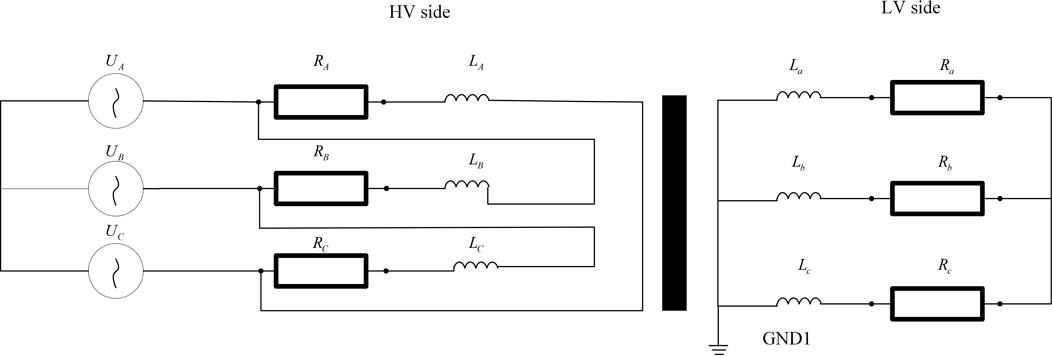
FIGURE 1. Power transformer circuit simulation topology.
2.2 Analysis of the influence factors of transformer acoustic signal under different voltage levels
The acoustic signal of transformer winding is generated under the action of electromagnetic force and transmitted to the surface of oil tank through fasteners and transformer oil. From the above analysis of the principle of winding vibration and sound generation, it can be seen that the main factors that affect the acoustic signal characteristics of transformers with different voltage levels are as follows:
1) The load current is different. When the voltage level is determined, it mainly depends on the capacity of the transformer. Obviously, the greater the load current flowing through the transformer during operation, the more significant the winding vibration signal.
2) Transformer winding structure. This is related to the inherent vibration characteristics of the transformer body. For a vibrating body, the magnitude of its vibration response actually depends on the excitation (voltage or current) and the inherent mechanical characteristics of its structure. Under the condition that the excitation is determined, the vibration response is closely related to its inherent mechanical characteristics, while the inherent mechanical characteristics of the transformer body are affected by its winding mechanical structure and fastening method and degree.
2.3 Analysis of signal characteristics of transformer winding during normal operation and short circuit
Through the analysis of the frequency domain data of the power transformer acoustic signal, it can be seen that the main component of the winding acoustic signal during the regular operation of the transformer is the even frequency multiplication component of 50 Hz. The odd frequency multiplication component is less, mainly based on the fundamental frequency of 100 Hz. As shown in Figure 2, the acoustic signal frequency of the winding during regular operation of the transformer is mainly 100 Hz, 200 Hz, etc.,
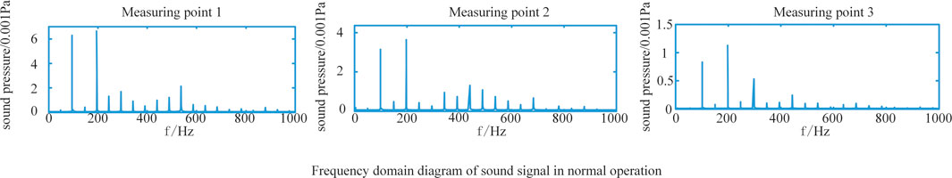
FIGURE 2. Frequency distribution of acoustic signal in normal operation of transformer winding.
When the transformer winding is a short circuit, because the acoustic vibration signal has a great relationship with the current flowing through the winding, when the current suddenly increases, it will generate greater electromagnetic force under the interaction with the leakage magnetic field. This electromagnetic force will aggravate the winding vibration and thus affect the acoustic signal of the transformer body. When a transformer in regular operation suddenly has a two-phase short circuit, its winding vibration acceleration is significantly higher than that in regular operation. At this time, the winding will be subject to quick circuit impact effect. When the transformer is subject to a short circuit impact, the winding will be slightly deformed. If it is not handled in time, fasten the pressing nails of the winding and the pull plates and pull rods of the iron yoke, and strengthen the clamping force of the leads. After several short circuit impacts, Due to the cumulative effect, the winding will still be unstable. Figure 3 shows the frequency domain diagram of the short circuit in phases ab, ac, and bc of windings.
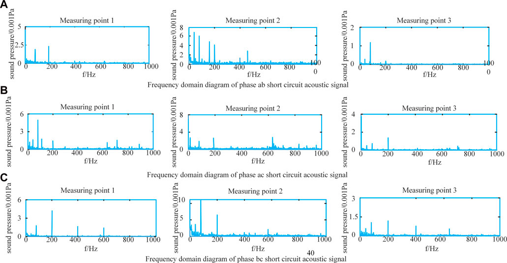
FIGURE 3. Frequency distribution of acoustic signal in two-phase short circuit of transformer winding.
It can be seen from the frequency domain analysis results in Figure 3 that when two phases of the winding are short-circuited, the frequency distribution of the acoustic signal of the winding is mainly within 1000 Hz. The amplitude size and frequency distribution of the acoustic signal displayed by the acoustic signals between different phases are not entirely the same. The frequency characteristics are relatively complex, and there is no definite change rule. The frequency is generally characterized by a high content of low-frequency components, and the frequency distribution is mainly below 1000 Hz.
3 Feature selection based on WKPCA-WM
3.1 Feature extraction of transformer acoustic signal based on WPES and MFCC
3.1.1 Acoustic signal feature extraction based on WPES
According to the theory of wavelet packets, there are generally three steps to decompose the transformer acoustic signal: Wavelet packet decomposition of the acoustic signal, calculation of interval energy of each frequency band, and construction of characteristic parameters (Saleh and Rahman, 2005).
Figure 4 below is a schematic diagram of three-level wavelet packet decomposition.
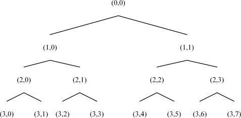
FIGURE 4. Three-layer wavelet packet decomposition diagram.
In the schematic diagram,
Step 1:. Perform three-layer wavelet packet decomposition on the transformer acoustic signal, extract the signal characteristics of eight frequency components in the third layer from low to high, and name the coefficients of the third layer as
Step 2:. Calculate the total energy of signals in each frequency band. If
Among them,
Step 3:. Construct the eigenvector and arrange the eigenvectors
Generally speaking, the value
The process of extracting characteristic parameters of wavelet packet energy spectrum of transformer sound signal is shown in Figure 5.Three-layer wavelet packet decomposition of the transformer sound signal can extract the energy characteristics in each frequency band. Assuming the frequency amplitude is 1000 Hz, for a more intuitive explanation, the frequency range of the third-layer reconstructed signal is given as shown in Table.1.
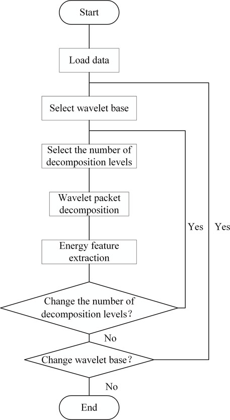
FIGURE 5. Flow chart for extracting characteristic parameters of wavelet packet energy spectrum of transformer sound signal.
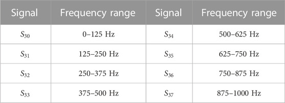
TABLE 1. Frequency range of the third layer reconstruction signal of transformer acoustic signal.
3.1.2 Acoustic signal feature extraction based on MFCC
The acoustic signal feature extraction MFCC algorithm based on MFCC has been widely used in speech recognition (Rieger et al., 2014) and fault diagnosis (Li et al., 2014). Therefore, this paper constructs the transformer voiceprint feature extraction method by referring to the MFCC feature extraction steps.
The specific MFCC parameter extraction process of the transformer acoustic signal is as follows:
3.1.2.1 Pretreatment
3.1.2.1.1 Preemphasis
The first-order high pass filter is generally used for pre-emphasis, and the transformer acoustic signal after pre-emphasis processing is set as
Where:
3.1.2.1.2 Endpoint detection
If a short-time acoustic signal is
The calculation formula of its short-time zero-crossing rate
Where
3.1.2.1.3 Framing
When processing a complete transformer sound signal, it is first divided into several frames, and then analyzed using the static process analysis method. To ensure continuity and smoothness between frames, the structure is moved for 10 ms to ensure the coincidence between boundaries.
3.1.2.1.4 Windowing
If the frame signal is
At present, Hamming Window is commonly used. Its formula is:
3.1.2.2 fast Fourier transform
Perform a fast Fourier transform on each frame of the transformer acoustic signal and calculate its spectral line energy:
3.1.2.3 Frequency filtering of transformer acoustic signal
To calculate the energy in the TSS filter when the spectrum of each frame passes through the TSS filter is actually to multiply and add the spectral line capacity
Where:
3.1.2.4 Discrete cosines transform (DCT)
The logarithm of the energy calculated in Step 3 is taken first, and the TSS spectral coefficients obtained are all real numbers. Then DCT is used to convert the TSS spectral coefficients to the domain, and the standard cepstrum coefficients based on the TSS frequency are finally obtained, with the formula as follows:
Where:
From the step of MFCC coefficient extraction, the most critical parameter is the number of transformer acoustic signal filters. Since the frequency of the transformer acoustic signal is mainly concentrated in the frequency doubling of 100 Hz, and the number of filters should not be too small, the number of filters selected is 40.
3.2 Feature extraction method based on WPES-MFCC
After wavelet packet energy spectrum decomposition, each frame of transformer sound signal can be expressed as a 32-dimensional feature vector, while each frame after MFCC extraction is a 40-dimensional feature vector. On the one hand, these two eigenvectors have relatively large dimensions and are more redundant when combined; On the other hand, studies have shown that the use of DCT in the calculation of MFCC parameters results in different contributions of each dimension of MFCC parameters to the recognition results (Ke et al., 2014). It is considered to combine the wavelet packet energy spectrum with the features in MFCC that have a large contribution to the fault diagnosis results to obtain the feature parameters with rich and accurate feature information and low redundancy, effectively improving the accuracy and speed of fault diagnosis and avoiding the disaster of dimensionality.
3.2.1 Feature dimension reduction based on WKPCA
KPCA (Shi et al., 2016) is a non-linear generalization of principal component analysis (PCA) (Aminullah et al., 2020). Through non-linear transformation
KPCA’s dimension reduction steps for the characteristics of transformer acoustic signals are as follows:
1) For the sample matrix
Where:
2) The eigenvalues and eigenvectors of the covariance matrix are
3) Define the matrix
Where:
WKPCA, an algorithm for feature dimensionality reduction of transformer acoustic signals, is obtained by introducing a weight factor. The eigenvalues are arranged in ascending order, and the feature vectors are also changed accordingly. According to the relationship between the principal components representing the original signal features, the first ten dimensional feature elements of the cumulative contribution rate are the critical feature parameters of transformer acoustic signals.
3.2.2 Feature selection based on WPES-MFCC
Firstly, calculate the cumulative contribution rate of wavelet packet energy spectrum and MFCC. The cumulative contribution rate of wavelet packet energy spectrum features is shown in Figure 6A, and the cumulative contribution rate of MFCC features is shown in Figure 6B.
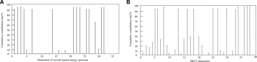
FIGURE 6. Cumulative contribution rate of wavelet packet energy spectrum and MFCC.
It can be seen from Figure 6 that although the cumulative contribution rates of wavelet packet energy spectrum and MFCC feature parameters are different, the existing problem is that the cumulative contribution rates of some important feature dimensions are the same, so it is difficult to separate their first 10 dimensional feature parameters.
The total cumulative contribution rate is obtained by weighting the cumulative contribution rate of WPES and MFCC. The ranking of characteristic parameters varies with the introduced weighting factors
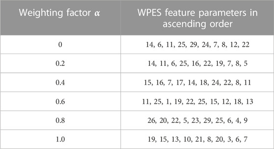
TABLE 2. The ascending order of WPES comprehensive characteristic parameters.
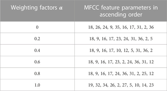
TABLE 3. Ascending ranking of MFCC comprehensive characteristic parameters.
It can be seen from Table.2 that the viscosity between WPES feature parameters is large, the importance of each feature parameter is not different, and the feature selection is greatly affected by the expected weight factor
The 10-dimensional WPES characteristic parameters
In this paper, the characteristics whose incremental contribution rate is higher than 95% are taken as the main parameters. It can be seen from Figure 7 that the cumulative contribution rate obtained by different weight factors is higher than 95%. However, when the weight factor
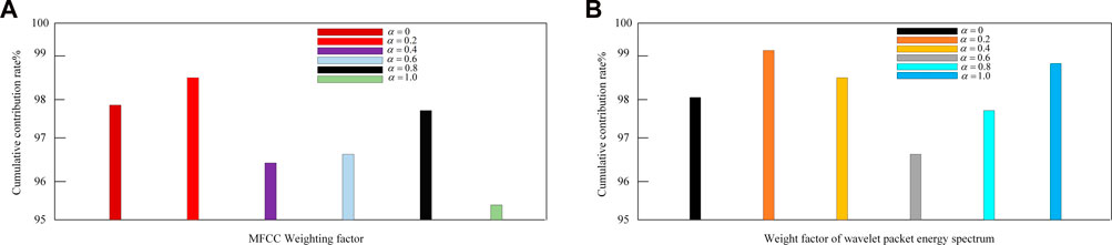
FIGURE 7. Cumulative contribution rate of WPES and MFCC comprehensive characteristic parameters with different weight factors.
When the weight factor value is 0.2, the complete feature parameters reach the optimal value, as shown in Figures 8A, B when the WPES comprehensive feature cumulative contribution rate and MFCC comprehensive feature cumulative contribution rate are, respectively.
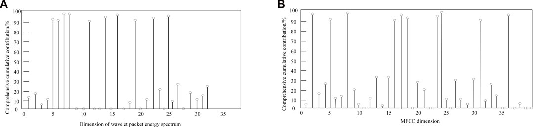
FIGURE 8. Cumulative contribution rate of comprehensive characteristic parameters of weight factor
4 Diagnosis model of transformer winding short circuit with voiceprint
Taking the optimal characteristic parameters as the input of the deep learning model can not only improve the network performance, but also significantly improve the computing speed. The convolution kernel of the convolution layer in the original CNN network is a standard convolution kernel, which cannot directly obtain the features of an extensive range, and lacks the adaptability to the changes in object shape and attitude; In addition, when the number of features channels becomes more extensive, the convolution kernel parameters become more prominent, which will increase a lot of computational overhead. Therefore, this paper proposes a new intelligent optimization algorithm for the convolution kernel of CNN. The Pelican optimization algorithm is used to train the convolution kernel of the convolution neural network to find the best convolution step size. The size of the optimized convolution kernel is prepared by the convolutional neural network to achieve multiple iterations of the CNN, so the diagnostic model gradually converges.
4.1 Basic unit model of convolutional neural networks
The convolutional neural network has strong adaptability, and is good at local mining data features, extracting global training features, and classification. CNN structure consists of the input layer, convolution layer, pooling layer, whole connection layer, and output layer.
The convolution operation is an integral part of a convolutional neural network. The convolution operation consists of two parts, one is the input parameter, and the other is the convolution kernel function. Output feature mapping is a parameter after convolution calculation. It can be seen from Figure 9 that the convolution calculation process and matrix multiplication have similar but different principles. This close connection between input and output is called a full connection. Still, the too dense a connection will lead to an increase in the amount of computation, which will cause specific difficulties in the training and learning of neural networks. The local sensing function of the convolutional neural network makes its input and output interact locally, which is a sparse connection. The schematic diagram is shown in Figure 9.
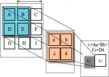
FIGURE 9. Schematic diagram of the convolution operation process.
In Figure 10, the gray line represents the whole connection of the traditional neural network, and the red line represents the sparse connection of the local perception of the convolutional neural network. The local perception function of the convolutional neural network can efficiently extract signal features from the noisy power transformer acoustic signals. Its meaningful features are only detected by smaller convolution kernels, which also make the stored parameters less, thus improving the computational efficiency of the model. As shown in Figure 10, when the convolutional neural network represented by the red and green lines is sparsely connected, the input parameters “B” and “C” are shared parameter sets. This feature is called parameter sharing. That is, the same convolution core shares the same convolution value and offset term. Parameter sharing eliminates the need to learn a set of individual parameters for each location, which makes the convolutional neural network more concise and efficient in model learning and parameter training.
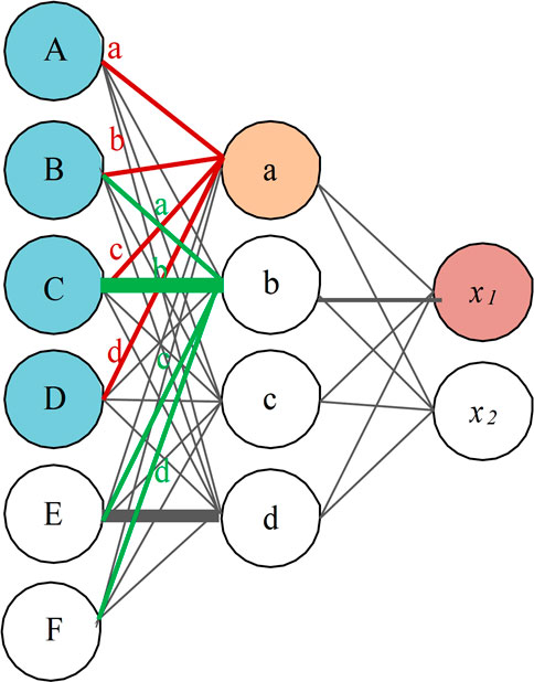
FIGURE 10. Schematic diagram of sparse connection in convolution process.
Pooling is also an essential level in convolutional neural networks. The pooling process mainly refers to the “secondary processing” of features extracted from the convolutional layer through the pooling function. The pooling process of a convolutional neural network has the advantages of feature extraction invariance, dimension reduction sampling characteristics, and effective prevention of overfitting. Based on convolution, the weak features of power transformer vibration signals can be further optimized, screened, and extracted. Commonly used pooling functions include the average pooling function and the maximum pooling function. The full pooling function used in this paper is shown in the following Eq. 24.
Where,
It can be seen from Formula (24) that the pooling operation is to divide the characteristics of the acoustic signal of the power transformer output from the convolution layer into pooling areas of size
The back-propagation algorithm in the convolutional neural network is one of the characteristics that convolutional neural network is superior to the traditional neural networks. The formal neural network training process is mostly a one-way forward transmission of “input parameters—raining and learning—classification processing—output results” one by one, which will make the output results have a significant deviation. At the same time, the back-propagation algorithm in the convolutional neural network is similar to the feedback link in the motion control system. When the input power transformer sound signal propagates forward in the convolutional neural network model, the back-propagation can allow the cost function to reverse propagate the error through the network structure, and update the gradient calculation. The back-propagation algorithm in a convolutional neural network can minimize the feature extraction error of the power transformer acoustic signal, and it can correct the error of the extracted feature, providing the maximum guarantee for better learning, training, and accurate identification of power transformer winding short circuit.
4.2 POA algorithm
The Pelican optimization algorithm (POA) (Trojovský and Dehghani, 2022) has high reliability and consistency, has strong optimal solution ability, and can be optimized with fast acceleration convergence and strong stability. Pelican optimization algorithm steps are as follows:
4.2.1 Initialize
The mathematical description of Pelican population initialization is as follows:
Where:
In the Pelican optimization algorithm, the pelican population can be represented by the matrix of Eq. 26:
Where:
Where:
4.2.2 Stage I: Approaching prey (exploration stage)
In the first stage, the pelican determines the location of its prey, and then moves to this determined area. Model it as follows:
Where:
In the POA algorithm, if the objective function value is improved at this part, the new position of the pelican is accepted. In this type of update, also known as an effective update, the algorithm cannot move to the non-optimal region. This process can be described by the following formula:
Where:
4.2.3 Phase II: Surface flight (development phase)
In the second stage, when the pelicans reach the water’s surface, they spread their wings on the water’s surface, move the fish up, and then put their prey in their throat bag. Modeling this behavior process of the pelican can make the POA algorithm converge to a better location in the hunting area, which increases the local search ability and development ability of the POA algorithm. This behavior of pelicans during hunting is mathematically modeled as follows:
Where:
When the development phase is over, the target function value of the new location will be updated. The updated formula as follows:
4.3 Sobol sequence initialization population
The distribution of initial solutions in the solution space of the swarm intelligence algorithm will significantly affect the convergence speed, and optimization accuracy of the algorithm, and the initial solutions with uniform distribution will help to improve the performance of the algorithm. The standard POA uses random numbers to initialize the population, and the distribution of the initial population is relatively uneven. In this paper, the Sobol sequence is used to initialize the population. To compare the spatial distribution of random numbers generated by random distribution and Sobol sequence (Duan and Liu, 2022), a random number distribution diagram of 500 population in two-dimensional space is generated within the range of [0,1]. From the comparison in Figure 11, it can be seen that the population distribution obtained by the Sobol sequence is more uniform and covers the solution space more thoroughly.
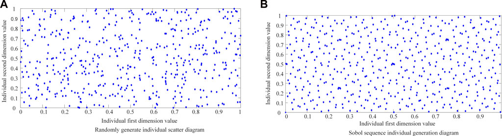
FIGURE 11. Distribution of individuals generated by random method and Sobol sequence.
This paper compares IPOA with POA, BOA, GWO, GSA, PSO, and ABC based on the same population size, maximum number of iterations and running times, as shown in Figure 12.
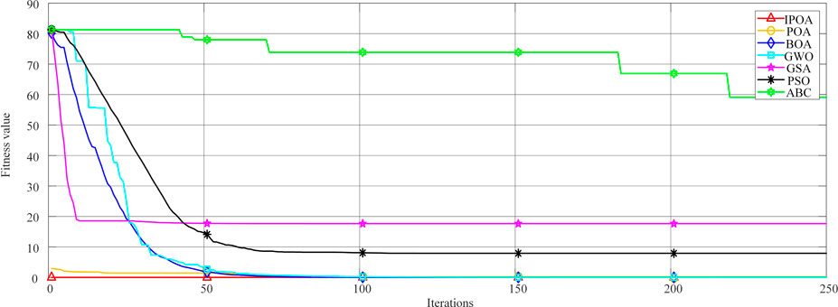
FIGURE 12. Comparison of performance between IPOA and different optimization algorithms.
For the two stages of POA, we need to judge the minimum value of the objective function of the two stages, to update the parameters. As seen from Figure 11, under the same population size, the maximum number of iterations, and the number of runs, the fitness value of IPOA is the minimum. That is, the error is the minimum. Compared with other algorithms, the fitness of IPOA is optimal.
4.4 Flow chart of transformer winding short circuit diagnosis based on WKPCA-WM and IPOA-CNN
As an essential parameter of CNN, the convolution kernel directly affects the accuracy and stability of the transformer winding short-circuit diagnosis model. Input the convolution step of CNN into the IPOA algorithm, and set the objective function as the judgment basis to calculate the convolution step with the best diagnosis performance through iterative optimization. WKPCA-WM and IPOA-CNN training flow chart is shown in Figure 13. The detailed steps are as follows:
1) WM characteristic parameters are input into the convolutional neural network.
2) Pelican optimization algorithm is used to train the convolution kernel of the convolution neural network to find the best convolution step. First, the Sobol sequence is used to optimize the initial population and determine the population size
3) The optimized convolution kernel size is trained by the convolutional neural network, and the numbers are input into the convolution layer, pooling layer, and top connection layer in turn. Convolution neurons can extract mixed features of training data.
4) The output loss function is calculated, and the weight value is updated through the gradient descent principle to achieve multiple iterations of CNN, so the diagnostic model gradually converges.
5) After several iterations, the test data set is used to judge the generalization ability and diagnostic ability of WKPCA-WM and IPOA-CNN.
6) According to the diagnosis results, the number of nodes, iteration times, lose value, and other parameters used in the neural network are adjusted.
7) Repeat steps (2–6) until the WKPCA-WM and IPOA-CNN models with the best performance for transformer winding short-circuit diagnosis are obtained.
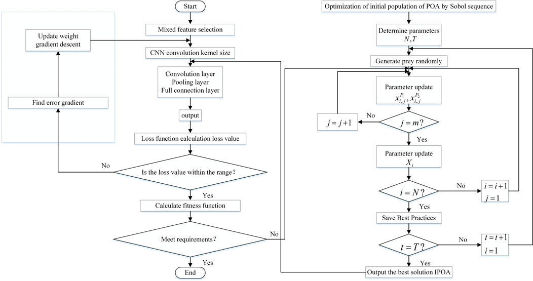
FIGURE 13. Transformer winding short circuit diagnosis model of WKPCA-WM and IPOA-CNN.
5 Experimental verification
5.1 Transformer acoustic signal acquisition test platform
The test platform mainly collects the acoustic signals of different two-phase short circuits of power transformer windings and the acoustic signals of the body during normal operation. The specific experimental acquisition scheme is as follows: arrange relevant measuring points on the front, side and top of the body surface of a practical transformer; Collect the acoustic signal of a two-phase short circuit of winding and the acoustic signal of the body of the power transformer during regular operation. The power transformer acoustic signal acquisition test platform based on the capacitive gun microphone is shown in Figure 14.

FIGURE 14. Transformer acoustic signal acquisition experimental platform.
The actual deployment of the simulation experiment for the established transformer winding short-circuit voiceprint diagnosis model is: Intel Core I7-6500U processor, the primary frequency is 3.1 GHz, 8G memory, and the Tensorflow environment is built in Python for model training and analysis.
5.2 Evaluating indicator
To test the accuracy and generalization of the WKPCA-WM and IPOA-CNN transformer winding short-circuit diagnosis models established in this paper. The accuracy of the test set is one of the evaluation indexes in this paper; Cross Entropy Loss (CE Loss) is introduced as the second quantitative evaluation index. Cross Entropy Loss depicts the distance between the actual output and the expected output of the established model. The objective function of the quantitative index is shown in Formula (32). For the two evaluation indicators, the higher the identification accuracy described in indicator 1, the more accurate the identification of the power transformer winding short circuit; The smaller the cross entropy loss related in indicator 2, the better the accuracy and robustness of the identification model.
In Formula (32):
In order to better evaluate and analyze the model established in this paper, this paper also introduces several kinds of indicators commonly used in machine learning to verify the model; the main indicators are sensitivity, F1-score and precision.
5.2.1 Sensitivity
In the classification task, the sensitivity rate refers to the recall rate of each category. Recall rate refers to the proportion of the predicted positive samples in the actual positive samples. Sensitivity rate is also called Recall rate. That is to say, the higher the sensitivity rate, the lower the corresponding probability of missing detection, and the more concerned is the probability of negative samples being detected. The specific calculation formula is as follows, that is, the ratio of the diagonal value of each column of the confusion matrix to the sum of all the values of this column:
5.2.2 Precision
In classification tasks, precision refers to the accuracy of each category. When evaluating the overall precision of the model, it is usually obtained by calculating the precision of each category first, and then weighted average. The precision rate refers to the proportion of the actual positive samples in the positive samples predicted by the model to the positive samples predicted. The higher the precision rate, the lower the corresponding false detection probability, that is, the more concerned about the classification precision of the positive samples. The calculation formula is as follows: The ratio of the diagonal value of each row of the confusion matrix to the sum of all values of that row:
5.2.3 F1-Scoe
F1-score is the harmonic average of precision rate and sensitivity rate, and the calculation formula is:
5.3 Analysis of experimental results
Based on the same experimental environment and experimental data, this paper takes LR = 0.01 as the optimal learning rate. It conducts comparative experiments on WKPCA-WM and IPOA-CNN models, CNN-LSTM models, and CNN models. The comparative analysis results of the three models are shown in Table 4. After calculation, the sensitivity, F1-score and precision results under different models are shown in Table.5.
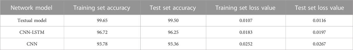
TABLE 4. Analysis of comparison results of different model experiments.
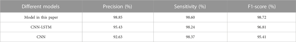
TABLE 5. Precision, sensitivity and F1-Score of different models.
It can be seen from Table.4 that WKPCA-WM and IPOA-CNN power transformer winding short circuit identification models have been established based on the idea of deep learning. The identification accuracy of both the training set and the test set is higher than that of CNN-LSTM and CNN models, and the accuracy of test set is 3.25%∼6.14% higher than that of the other two models. Its cross-entropy loss value is also smaller than the other two commonly used single models, and the loss value is 0.0081∼0.0151 smaller than the other two models. The result of the confusion matrix identification is shown in Figure 15.
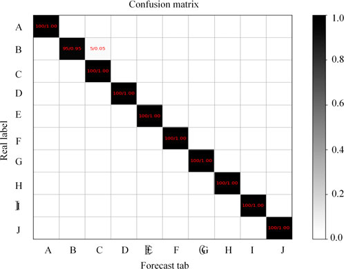
FIGURE 15. Disturbance matrix of transformer sound winding short circuit identification.
It can be seen from Table 5 that the transformer winding short circuit voiceprint recognition model established in this paper has its own advantages in different indicators. First of all, in terms of accuracy, the error detection rate of the model in this paper is low when identifying faults, while for CNN-LSTM and CNN models, the accuracy rate is low; Secondly, in terms of sensitivity, the error rate of the three models is basically the same, but in terms of the final comprehensive classification rate, the model in this paper performs better, and the F1-Score of the other two models is relatively low. Therefore, no matter from the accuracy rate and the cross entropy loss value.
In this paper, the confusion matrix is used to measure the recognition result of the model on the samples. The proposed model can effectively identify the short winding circuit, with an average recognition rate of 99.5%.
The comparison results of diagnostic accuracy and a cross-entropy loss of the three models in the training process are shown in Figures 16, 17.
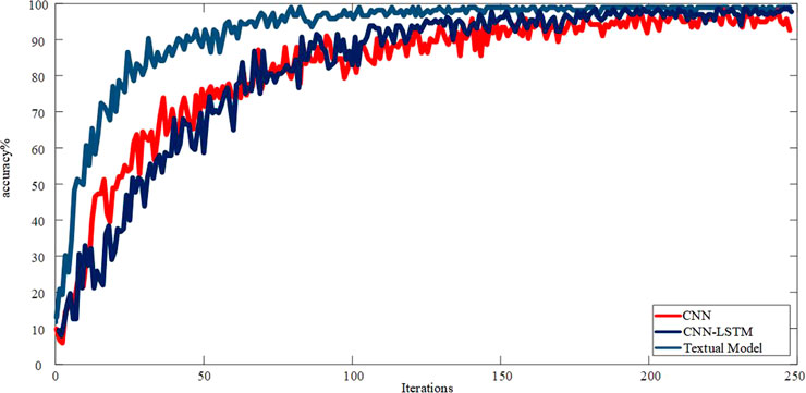
FIGURE 16. Comparison of accuracy results of different model training processes.
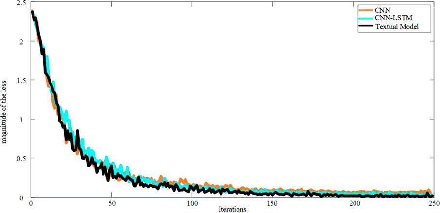
FIGURE 17. Comparison chart of cross entropy loss results in different model training processes.
The test set is used to verify the generalization ability of the transformer winding short-circuit diagnosis model based on the WKPCA-WM and IPOA-CNN. Through the verification of the test set, the diagnostic accuracy of WKPCA-WM and IPOA-CNN models is higher than the other two commonly used models. From the results of the evaluation indicators, the performance of the transformer winding short-circuits identification model established in this paper is better than the other two models. It can be seen from Figure 16 that, with the increase in the number of training iterations, the recognition accuracy is gradually rising, and the diagnostic accuracy of the model is rising faster than the other two models. After about the 200th iteration, the recognition accuracy reaches the superior value and tends to be stable, and the convergence of the model is also more robust than the other two models.
It can be seen from Figure 17 that with the increase of training iterations, the loss rate of the model decreases gradually. Among them, the loss values of the WKPCA-WM and IPOA-CNN models consistently declined in 250 iterations until they reached a stable state, and the models performed well. In transformer winding short circuits diagnosis, WKPCA-WM and IPOA-CNN models based on deep learning have high precision diagnosis ability and excellent generalization ability.
6 Conclusion
In this paper, transformer winding short-circuit acoustic signal is taken as the research object. Using the transformer winding short-circuit acoustic signal data collected in the laboratory, and based on WKPCA-WM and IPOA-CNN, a two-phase short-circuit acoustic signal diagnosis model of the transformer winding is established. The main conclusions are as follows:
1) A feature selection method of transformer acoustic signal based on WM is proposed. Through the combination of two different algorithms and according to the characteristics of transformer winding acoustic signal, more suitable feature parameters are selected. Compared with a single feature extraction algorithm, it has better noise immunity.
2) WKPCA is used to reduce the dimension of WM features, sort and select the selected high-dimensional features, and select the first 20-dimensional features that are more representative and can better reflect the acoustic signal of transformer windings, which effectively solves the problem of high feature redundancy and extensive calculation caused by the combination of the two methods; Secondly, by constructing a new comprehensive feature parameter as the input of the deep learning model, not only the performance of the model can be improved, but also the recognition accuracy of fault diagnosis can be improved.
3) The CNN network is optimized by IPOA. First, the Sobol sequence is used to optimize the initial population of POA, and then the optimal convolution kernel of the model in this paper is obtained by optimizing the convolution kernel, which makes the model have better diagnostic accuracy
4) The transformer winding short-circuit voiceprint diagnosis model based on WKPCA-WM and IPOA-CNN is constructed, and the CNN-LSTM and CNN algorithms are compared. The results show that the diagnosis model built in this paper is more accurate in the diagnosis accuracy within the same iteration number, and tends to be stable when the iteration number reaches 200. After 250 iterations, the accuracy of winding short-circuit fault diagnosis reaches 99.50%, the accuracy rate also reached 98.85%, the sensitivity reached 98.60%, and the F1-Score reached 98.72%, The validity and accuracy of the model are verified.
The paper explains the factors that affect the acoustic signals of transformer windings under different voltage levels, which are mainly determined by the load current and winding structure. However, due to incomplete data acquisition, the acoustic signals of transformers with different voltage levels have not been compared and analyzed one by one, mainly for a 10 kV power transformer. In addition, because the actual condition of the measured transformer is not known, besides the voltage level, the operating life the structure of the transformer will affect the characteristics of the acoustic signal. Therefore, it is necessary to continue to accumulate more measured data of acoustic signals in the future, and conduct more in-depth statistical analysis of the characteristics of acoustic signals of transformers in combination with the operation history of transformers and laboratory tests.
Data availability statement
The original contributions presented in the study are included in the article/supplementary material, further inquiries can be directed to the corresponding author.
Author contributions
HL: Methodology, algorithm finding, experimental platform provision, editing, supervision and review. DL: Algorithm finding, programming, simulation, writing-original draft preparation. YZ: Methodology, experimental platform provision, algorithm refinement, editing, supervision and review. YS: Methodology, algorithm search, raw data provision, review, article refinement. DF: methodology, algorithm refinement, editing, supervision and review. SS: Algorithm search, testing, validation.
Funding
This work was sponsored in part by the National Natural Science Foundation of China (52167014).
Conflict of interest
The authors declare that the research was conducted in the absence of any commercial or financial relationships that could be construed as a potential conflict of interest.
Publisher’s note
All claims expressed in this article are solely those of the authors and do not necessarily represent those of their affiliated organizations, or those of the publisher, the editors and the reviewers. Any product that may be evaluated in this article, or claim that may be made by its manufacturer, is not guaranteed or endorsed by the publisher.
References
Abbasi, A. R., and Gandhi, C. P. (2022). A novel hyperbolic fuzzy entropy measure for discrimination and taxonomy of transformer winding faults. Ieee Trans. Instrum. Meas. 71, 1–8. doi:10.1109/tim.2022.3212522
Ahn, H., Oh, Y., and Kim, J. (2012). Experimental verification and finite element analysis of short-circuit electromagnetic force for dry-type transformer[J]. Ieee Trans. Magnetics 48 (2), 819–822. doi:10.1109/tmag.2011.2174212
Aminullah, A., Mardiah, M., Hakim, L., Syahbirin, G., and Kemala, T. (2020). Spectra and carbonyl index changes on processed beef fats using Fourier transform infrared spectrometer and principal component analysis. Spectrosc. Lett. 53 (2), 114–122. doi:10.1080/00387010.2019.1700527
Arivamudhan, M., Santhi, S., and Abirami, S. (2014). “Improved detection sensitivity with combined WPT and HHT for power transformer winding deformation analysis[C],” in Proceeding of the Foundation of Computer Science (FCS).
Beckham, R., Karami, H., and Naderi, M. S. (2022). Application of artificial neural network on diagnosing location and extent of disk space variations in transformer windings using frequency response analysis[C], 30th International Conference on Electrical Engineering (ICEE) (Ieee), 1079–1084.
Bigdeli, M., and Abu-side, A. (2022). Clustering of transformer condition using frequency response analysis based on k-means and Goa. Electr. Power Syst. Res. 202, 107619. doi:10.1016/j.epsr.2021.107619
Bjelić, M., Brković, B., Žarković, M., and Miljkovic, T. (2022). Fault detection in a power transformer based on reverberation time. Int. J. Electr. Power & Energy Syst. 137, 107825. doi:10.1016/j.ijepes.2021.107825
Borucki, S. (2012). Diagnosis of technical condition of power transformers based on the analysis of vibroacoustic signals measured in transient operating conditions. Ieee Trans. Power Deliv. 27 (2), 670–676. doi:10.1109/tpwrd.2012.2185955
Duan, Y., and Liu, C. (2022). Sparrow search algorithm based on Sobol sequence and cross strategy. J. Comput. Appl. 42 (1), 36.
Ezziane, H., Houassine, H., Moulahoum, S., and Chaouche, M. S. (2022). A novel method to identification type, location, and extent of transformer winding faults based on FRA and SMOTE-SVM. Russ. J. Nondestruct. Test. 58 (5), 391–404. doi:10.1134/s1061830922050047
Islam, S., and Abusiada, (2015). Improved power transformer winding fault detection using FRA diagnostics – part 1: Axial displacement simulation. Ieee Trans. Dielectr. Electr. Insulation a Publ. Ieee Dielectr. Electr. Insulation Soc. 22 (1), 556–563. doi:10.1109/tdei.2014.004591
Ke, J., Zhou, P., and Jing, X. (2014). The mixed parameters of differential and weighted Mel cepstrum are applied to speaker recognition. Microelectron. Comput. (9), 88–91.
Li, Z. T., Gao, Y., and Zhou, X. (2014). Feature extraction of faulty rolling element bearing based on time synchronous average and cepstrum edit[C]//Advanced materials Research. Trans. Tech. Publ., 666–670.
Rieger, S. A., Muraleedharan, R., and Ramachandran, R. P. (2014). “Speech based emotion recognition using spectral feature extraction and an ensemble of knn classifiers[C],” in 2014 9th International Symposium on Chinese Spoken Language Processing (ISCSLP) (Ieee), 589–593.
Saleh, S. A., and Rahman, M. (2005). Modeling and protection of a three-phase power transformer using wavelet Packet transform. Ieee Trans. Power Deliv. 20 (2), 1273–1282. doi:10.1109/tpwrd.2004.834891
Shi, H., Song, W., and Zhang, K. (2016). Fault detection method of kernel principal component analysis based on particle swarm optimization. [J] J. Shenyang Jianzhu Univ. Nat. Sci. Ed. 32 (4), 710–717.
Shi, Y., Ji, S., and Zhang, F. (2019). Multi-frequency acoustic signal under short-circuit transient and its application to condition monitoring of transformer winding [J]. Power delivery. Ieee Trans. doi:10.1109/TPWRD.2019.2918151
Tango, B. A., Nnachi, A. F., Dlamini, G. A., and Bokoro, P. N. (2022). A novel approach to assess power transformer winding conditions using regression analysis and frequency response measurements. J. Energies 15 (7), 2335. doi:10.3390/en15072335
Tarimoradi, H., Karami, H., Gharehpetian, G. B., and Tenbohlen, S. (2022). Sensitivity analysis of different components of transfer function for detection and classification of type, location and extent of transformer faults. Faults J. Meas. 187, 110292. doi:10.1016/j.measurement.2021.110292
Trojovský, P., and Dehghani, M. (2022). Pelican optimization algorithm: A novel nature-inspired algorithm for engineering applications. Sensors 22 (3), 855. doi:10.3390/s22030855
Xian, D., Zhang, B., and Liu, X. (2021). The transient characteristics of inter-turn short circuit in power transformer windings are analyzed by finite element method. [J] J. Mot. Control 25 (10), 130–138.
Zhang, Bingqian, Xian, Daidai, and Yang, Yu (2021). Analysis of physical characteristics of power transformer windings under interturn short circuit fault. J. High. Volt. Technol. 47 (6), 9.
Nomenclature
Keywords: voiceprint signal, feature selection, WKPCA-WM, pelican optimization algorithm, Sobol sequence, IPOA-CNN
Citation: Pei X, Han S, Bao Y, Chen W and Li H (2023) Fault diagnosis of transformer winding short circuit based on WKPCA-WM and IPOA-CNN. Front. Energy Res. 11:1151612. doi: 10.3389/fenrg.2023.1151612
Received: 26 January 2023; Accepted: 06 March 2023;
Published: 24 March 2023.
Edited by:
Zijun Zhang, City University of Hong Kong, Hong Kong SAR, ChinaCopyright © 2023 Pei, Han, Bao, Chen and Li. This is an open-access article distributed under the terms of the Creative Commons Attribution License (CC BY). The use, distribution or reproduction in other forums is permitted, provided the original author(s) and the copyright owner(s) are credited and that the original publication in this journal is cited, in accordance with accepted academic practice. No use, distribution or reproduction is permitted which does not comply with these terms.
*Correspondence: Songtao Han, MTM2OTE4Njk2OEBxcS5jb20=