 Zhihan Wu
 Yi Zhang*
- College of Electrical Engineering and Automation, Fuzhou University, Fuzhou, Fujian, China
A short-term prediction method for distributed PV power based on an improved selection of similar time periods (ISTP) is proposed, to address the problem of low output power prediction accuracy due to a large number of influencing factors and the large difference in the degree of influence of various factors. First, the simple correlation coefficient (SCC) based on path analysis is used to screen the main influencing factors with stronger correlation with PV output power, and these factors are classified into three categories. Second, correlations of the three dimensions are calculated, respectively: (i) TOPSIS (with weights optimized by the SCC) determines meteorological correlation, (ii) linear weighting (based on the fuzzy ranking) obtains time correlation, and (iii) load correlation is quantified with existing current parameters. Third, the combined impact correlation (CIC) is obtained by weighting the three correlations above to establish criteria for the selection of similar periods, and a short-term PV power prediction model is established. Finally, experimental results based on real data of Australian Yulara Solar System PV plant demonstrate that errors of proposed ISTP method are respectively improved by 47.06% and 46.09% compared with the traditional ELMAN and similar day method.
1 Introduction
With the goal of the promotion of China’s “double carbon” and the continuous development of technology, photovoltaic power generation has rapidly become the third largest renewable energy source after hydropower and wind power (Sheng et al., 2019). However, output power of distributed PV power plants is highly intermittent and random. Therefore, accurate forecasting of PV power generation is significantly important to stabilize and secure grid operation and promote large-scale PV power integration (Utpal et al., 2018).
In recent years, a great deal of research on improving the prediction accuracy of photovoltaic power has been carried out to reduce the uncertainty in forecasting (Antonanzas et al., 2016). In the current studies, there are two main approaches that are widely used in the forecasting of PV system production: Indirect and direct (Kıvanç et al., 2020). Compared with indirect prediction, direct prediction can effectively improve the model accuracy due to the introduction of actual historical data of PV power plant output to calibrate the mechanistic model accordingly; but it requires analysis of a large amount of historical power generation data. For this reason, existing studies introduce the concept of a similar historical day (whose PV output power is similar to the power of the day to be predicted) to significantly reduce the amount of data required. The literature (Wu et al., 2022; Chen et al., 2017; Niu et al., 2020) mention the use of meteorological features to screen similar days as input samples to the model for direct prediction. Direct prediction based on similar days is a relatively simple and feasible method in short-term prediction. Also in the field above, the solar radiation intensity is often selected as a screening criterion for similar days after correlation analysis (Zhu et al., 2018; Ge et al., 2021; Zhang et al., 2021). Existing similar day methods (Fu et al., 2012; Sun et al., 2013; Wang and Ge, 2013; Luo et al., 2018) mostly study the overall similarity between a historical day (day before the forecast date) and the day to be predicted. They usually classify the historical data, and choose the highest, the lowest and the mean value of various influencing factors in one day. The values above (representing only one point in time) are often weighted to represent the overall data of entire day (without an in-depth analysis of differences in the degree of influence of each factor at different time periods).
For this reason, researchers have proposed a number of forecasting methods that analyze similar time period. (a) The literature (Lu et al., 2017; Li et al., 2018) propose integrated forecasting methods where the meteorological types were classified and then they adopted different methods to predict smooth and fluctuating PV output, respectively. However, due to the limitation of the small data sample size, such methods do not eliminate heterogeneous data and lead to a large amount of redundant information input to the model. Furthermore, this will result in long training time, poor accuracy, and adaptability of the model. (b) The literature (Cheng et al., 2017) uses K-means to screen and cluster the historical samples and then estimates PV output probability distribution by kernel density. The correlation analysis of the data reduces the dimensionality while eliminating heterogeneous data, which improves the prediction results. Howerver, the weights of each meteorological factor are not further determined in the similarity analysis. (c) To study the method of determining the weights of each factor, the literature (Peng et al., 2019) corrects the meteorological data by clustering. They design a comprehensive measure to find the optimal set of similar time periods and uses ELMAN model for forecasting. The literature (Tan et al., 2021) adopted path analysis to determine the weights and calculated comprehensive factor correlation of each time period. They quantified the meteorological, load, and time factors respectively to realize the dynamic optimization of the number of similar time periods.
In summary, existing PV forecasting methods that improve accuracy through in-depth analysis of time have following two problems: (a) A large number of meteorological factors and PV output values are not screened before inputting them into the model, or the lack of condensed screening criteria makes the screening less targeted. Both can result in an insufficient number of similar time periods or weak correlation. (b) Due to the inherent defects of neural networks, problems such as overfitting and local optimization are likely to occur, resulting in a decrease in model prediction accuracy.
To address the problems above, we propose a short-term prediction method for distributed PV power based on improved similar time period (ISTP). Firstly, the simple correlation coefficient (SCC) based on path analysis is used as thresholds to screen main influencing factors with a stronger correlation with PV output power. They are classified into three categories: Meteorology, time, and load, to reduce the dimensionality of data. Path analysis can measure both direct and indirect coupling of each factor with PV output. Secondly, TOPSIS (with weights optimized by the SCC) determines meteorological correlation, linear weighting (based on the fuzzy ranking) obtains time correlation, and load correlation is quantified directly based on existing current parameters. Then correlation of the three dimensions above and the SCC are jointly weighted to obtain the combined impact correlation (CIC) as the similar time periods screening criteria. Finally, we carry out method validation based on Yulara Solar System PV plant in Australia. The validation results show that our method ensures strong correlation between similar time data and predicted output value by comprehensively considering influence of three dimensional factors. Also we achieve dynamic optimization of the screened similar time period quantity, which effectively improves the prediction accuracy. Table 1 explains the acronyms that appear in the paper.

TABLE 1. List of acronyms.
2 Fundamentals of path analysis
Interactions between different factors can affect PV power predction to different degrees. Such effect is not only reflected in direct influence of the factor itself on the prediction, but also in its indirect influence on the prediction through other factors. Therefore, we choose path analysis to calculate the SCC to comprehensively measure both direct and indirect effects in the interaction of factors.
2.1 Calculation method of the direct path coefficient (DPC)
The dependent variable y and n distinct independent variables x (x1, x2, …, xa, …, xn) all contain m sets of data. The DPC r1,a is calculated by using
In Eq. 1, a denotes the type of factor, xa,t is the sample t of influencing factor a, yt is the sample t of PV power y, m is the total number of selected days and ba denotes the bias regression coefficient.
2.2 Calculation method of the indirect path coefficient
First, we calculate correlation coefficient ra,a+1 between any two independent variables xa and xa+1 as
When combining the DPC and correlation coefficient calculated above, the indirect path coefficient r2a,a+1 represents indirect effect of factor a on output y through factor a+1, which is given by
2.3 Calculation method of SCC
Combining the two types of coefficients above, the SCC ra between xa and y is calculated by the following formula:
In Eq. 4, r2a,o denotes the indirect path coefficient of influencing factor a about another influencing factor o. This SCC indicates indirect influence of factor a on dependent variable (PV output y) through factor o.
By combining characteristics of two types of path coefficients, the SCC not only measures influence of the factor itself on prediction, but also captures influence of that factor on prediction through other types of factors.
3 Fundamentals of the CIC
Since there are many influencing factors of distributed PV power, we categorize eight influencing factors focused on research into three dimensions: (i) meteorological factor (ambient air pressure, ambient air temperature, wind level, total irradiance, scattered irradiance, and sensor operating temperature), (ii) load factor (average current), and (iii) time factor.
Firstly, the quantitative data of each influencing factor are obtained and the eight simple correlation coefficients are calculated in Section 3.1. Then the eight factors are screened to obtain strong correlation influencing factors and these strongly correlated factors are grouped into three categories. Next, time correlation, load correlation, and comprehensive meteorological correlation are respectively calculated in Section 3.2. Finally, three types of correlation above are linearly weighted with the simple correlation coefficients of path analysis to calculate the CIC, which measures the degree of influence of each factor on PV output in Section 3.3.
3.1 Data preprocessing of the three-dimensional factors
3.1.1 Quantification of the time factor
Since data are directly available for the two impact factors in (i) and (ii) except for the time factor in (iii), the quantification method of time factor data is first investigated to help subsequent heterogeneous data elimination and screening of main impact factors.
Because correlation between time factor and PV power may be reduced if the correlation is only directly measured by distance in time alone, we will improve the correlation between the time factor and PV power in two ways. This is done by (i) calculating ratio of PV average value of historical time periods to the total PV power value of whole day as the weight to represent PV power at each time period (ii) adopting the fuzzy ranking to calculate and using the results directly as quantitative data of time factor. The specific steps are as follows.
1) Use the average PV power at time period j of m sample days to measure the proportion of that time periods among the 11 periods of whole day as follows:
In Eq. 5, mij denotes PV power output at time period j in the day i, and Zj denotes the proportion of time j.
2) The m samples of time period j are sorted by power values from largest to smallest. When PV power attains the maximum value, a weight of m is assigned to Zj. When the second largest value is obtained, a weight of m-1 is assigned to Zj. This continues and when PV power attains the minimum value at a certain time, a weight of 1 is assigned to Zj. The quantitative data Nij of time factor is obtained by
In Eq. 6, hij denotes the weight value of each time period to be measured according to what we described above.
3.1.2 Calculation of the SCC
3.1.2.1 Definition of feature symbols
The characteristics studied in this paper include ambient air pressure, ambient air temperature, wind level, total irradiance, scattered irradiance, sensor operating temperature, average current, and time factor, for a total of eight factors that affect PV output. For the subsequent description, we write Sij, Tij, Dij, Hij, Wij, Gij, Pij, Nij, respectively, to donote each of eight factors at time period j on the day i (i = 0 indicates the day to be measured) before the day to be measured. Furthermore, m is the total number of historical days. Influencing factor symbols and corresponding names are shown in Table 2.
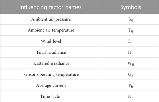
TABLE 2. Influencing factor symbols and corresponding names.
3.1.2.2 Data normalization
The influencing factors discussed above are normalized according to Eq. 7 below and the metric scales of different magnitudes of data are limited to a certain range to obtain eight feature matrices:
In Eq. 7, u = S, T, D, H, W, G, P, N, C is a constant, and uij is a type of influencing factor.
3.1.2.3 Calculation of the simple correlation coefficients of eight influencing factors
The daily average of the eight influencing factors from m historical days are calculated separately as independent variables. The daily average of PV power for the corresponding historical days is calculated as dependent variables. Then the simple correlation coefficients of each influencing factor above are calculated according to Section 2.1.
3.2 The correlation of the three-dimensional factors
The SCC of each influencing factor and the correlation parameters in three dimensions of time, load and meteorology are jointly linearly weighted to derive the CIC of historical effective output time periods Gij. Thus, we can obtain condensed similar time period screening criteria, which can ensure a strong correlation between similar time periods and corresponding time periods of the day to be measured so as to further improve the prediction accuracy.
3.2.1 Time correlation
The time factor data (quantified above with the help of the fuzzy ranking) has improved the correlation between time and the value to be predicted to some extent. In the next section, we will focus on the specific calculation method of this correlation.
The strength of the correlation is measured according to the principle of “big near and small far” in time, that is, the correlation is small if the time is far away from the date to be predicted and large if it is not. The temporal correlation bi is linearly portrayed using the temporal distance as follows:
In Eq. 8, i denotes the day i before the day to be predicted and bi denotes time correlation of day i.
Unlike the traditional method (which selects only according to the single criterion of temporal distance), we first quantify the temporal factors by the fuzzy ranking and then perform the further correlation analysis. This procedure can improve the correlation of both quantitative data and temporal factors with PV-predicted output values at the same time.
3.2.2 Load correlation
The trend of power plant output can be more accurately, completely and reliably reflected by the current curve. In Qiao et al., 2021, it is proposed that the current data of each power plant can be input into the model as a reference and the difference in power plant output can be continuously adjusted during the iteration process to achieve the optimization of deviation values. Given this, we use the magnitude of difference between average currents at any two time periods to measure the degree of correlation between the output of two time periods, the larger the difference the smaller the correlation, and vice versa. The correlation dij between the average currents of historical day i and the day to be predicted at the same time period j is calculated according to the following Eq. 9:
In Eq. 9, Pij denotes the average current of time period j on day i and Poj denote the average current of time period j of the day to be measured.
3.2.3 Meteorological correlation
3.2.3.1 Definition of baseline meteorological factors
From the discussion above, several major meteorological factors (which are used to characterize the meteorological properties) include ambient air pressure, ambient air temperature, total solar irradiance, scattered irradiance, and sensor operating temperature. What we do here is primarily inspired by the theory of TOPSIS and we use distance relationship existing between meteorological factors and optimal meteorological factors at any effective time period of historical day to obtain the main basis for the calculation of meteorological correlation.
TOPSIS is a common integrated assessment method that makes full use of the information from raw data. Consequently, the results of this method accurately reflect the differences of strengths and weaknesses between the different assessment options. The baseline meteorological factors are defined as indicated below:
In Eq. 10 and Eq. 11, TY is the optimal meteorological factor and Tc is the worst meteorological factor. Here, TY1, TY2,…, TY5 and TC1, TC2,…, TC5 represent, respectively, the optimal and worst distances between PV power and the five primary influencing factors (ambient air pressure, ambient air temperature, total irradiance, scattered irradiance, and sensor operating temperature).
3.2.3.2 TOPSIS optimized by the SCC
The traditional TOPSIS does not take into account the horizontal influence between factors when setting the weights. Here, we fully consider the intrinsic correlation level reflected by the distance between the selected meteorological factors and the defined optimal meteorological factors. We propose the optimized TOPSIS by using the SCC as the weight. That is, the larger the absolute value of the SCC of the influencing factor is, the closer the factor is to the optimal factor, which results in the stronger correlation with the actual results and a more significant influence on the prediction.
The positive distance MZij (obtained by optimizing the principle of TOPSIS) is calculated as follows:
In Eq. 12, r1, r2,…, r5 are, respectively, the simple correlation coefficients of ambient air pressure, ambient air temperature, total irradiance, scattered irradiance, and sensor operating temperature.
Similarly, the negative distance MFij is calculated as follows:
The proximity of the meteorological factors to the optimal meteorological factors at each effective time period is then calculated as follows.
In Eq. 14, 0 ≤ Mcij ≤ 1. Obviously, the smaller the positive distance MZij is, the larger Mcij is, that is, the closer to the optimal meteorological factor.
The integrated meteorological correlation between the similar days and the day to be predicted at each effective time period is calculated as below
In Eq. 15, Mcoj is the calculation results of the time periods to be predicted.
We use the difference between evaluation results of meteorological characteristics of the historical time period and the time period to be measured (Mcij and Mcoj) to measure the closeness of the two time periods. The closer the two time periods are, the greater the integrated meteorological correlation is, which indicates that the correlation between the meteorological data of the historical time period and the time period to be measured is stronger.
3.3 Calculation of the CIC
We use the calculated correlation of the three dimensions and the simple correlation coefficients of each factor linearly weighted to derive the CIC of each historical effective output time period. The condensed similar time period screening criteria is obtained and the CIC is calculated below:
In Eq. 16, rb and rd denote the simple correlation coefficients of the time factor and the load factor (average current), respectively.
The calculation flow of the CIC is shown in Figure 1.
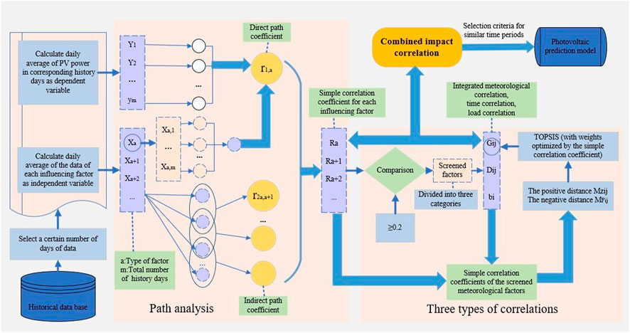
FIGURE 1. Technical route to obtain the CIC.
4 Prediction model based on ISTP
4.1 Establishment of the prediction model framework
We establish the prediction modal framework in the following five steps.
(1) Initialize to define GM as the limit value of the CIC and define NM as the minimum number of similar time periods. The historical time periods whose values of integrated impact correlation are greater than GM are defined as similar time periods. If the number of similar time periods selected based on their integrated impact correlation Gij is less than NM, then NM is taken to indicate the number of similar time periods at that time period and the lack of data is complemented by the average value of PV power at the selected similar time periods.
(2) Calculate the CIC Gij of each time period on the similar day to the forecast day.
(3) Calculate the number of time periods that satisfies Gij ≥ GM at time period j as below:
In Eq. 17, N is the final number of similar time periods according to the steps above and Nc is the number of similar time periods that satisfy the condition above.
(4) After the similar time periods are selected, PV power at time period j is first predicted using a weighting method based on the CIC as follows:
In Eq. 18, Tkj is PV power at time period j of day k before the day to be predicted (k ≠ i) and Gkj is the calculated CIC between time period j of day k before the day to be predicted and time period j of the day to be predicted.
(5) PV power at time period j is further predicted based on the extrapolation method. The final predicted value is the average of the results calculated by the two methods above. The parameters of T2j and Moj are calculated as follows.
4.2 Parameter initialization and determination of optimal parameters
Based on the previous analysis, the similar time period selection and PV power prediction process is given in Figure 2. The procedure is described as follows.
1) Using historical data, the ratio of data in the training set and the test set is set at 8:2 by referring to the ratio distribution of traditional machine learning small-scale data sets.
2) The true value is compared with the predicted value at each time period of the historical day and the relative error sum of squares is calculated as below:
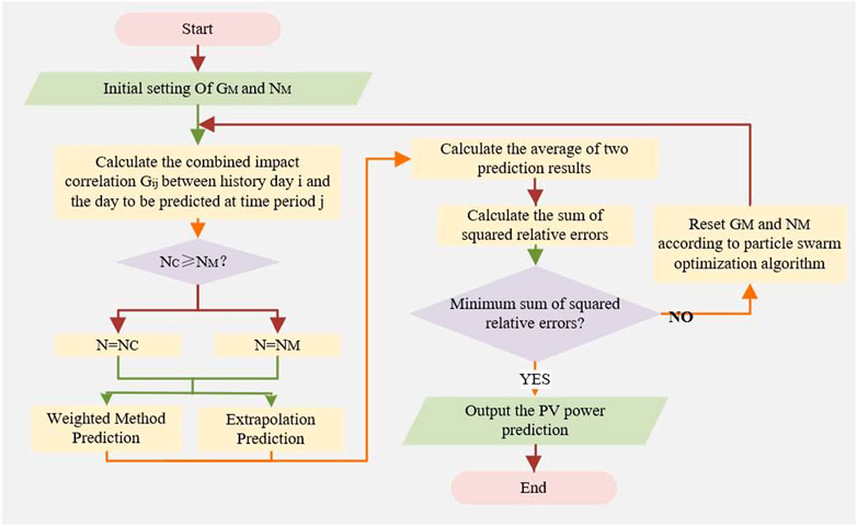
FIGURE 2. Photovoltaic power prediction flow chart.
In Eq. 21, MTj is the true PV power at time period j of historical day i (used as the parameter training sample).
3) When E(GM, NM) is smallest, the particle swarm optimization algorithm (Zhao et al., 2005) is used to find the corresponding optimal model parameters GM and NM.
4) Input the test set data into the model for PV power prediction and verify the effectiveness of the algorithm.
5) Input the calculated optimal parameters into the constructed prediction model framework to achieve PV power prediction.
5 Example analysis
5.1 Case study
We have selected the Yulara Solar System PV plant in Australia as the actual measurement object to verify the proposed method’s effectiveness. A total of 90 historical days of data from June to August in one-quarter are selected as samples. The daily power measurement time interval is from 08:00 to 19:00 and the data are collected at a 5-min interval. Thus, each historical day has 132 effective power output time periods. Figure 3 illustrates the PV output power database. Note that while training on more data is almost certainly going to yield better results, the anticipated performance increase would probably be quite minor at the expense of significant additional training time (Zhang et al., 2018). We thus consider these days as a representative sample of the entire dataset.
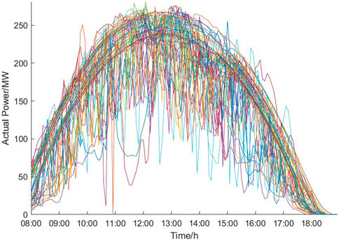
FIGURE 3. 90-day PV output power database.
As can be seen from Figure 3, it is difficult to obtain overall similar curves using the similar day method because the curves only partially overlap or intersect. It means that the PV output power is exactly the same in the periods where the curves intersect. Therefore, it is more likely to obtain high similarity by analyzing the periods.
PV power prediction effect is described by calculating PV power prediction error (that is, the error relative to the actual power) of ISTP. PV prediction results are evaluated using the root mean square error (RMSE) and the mean absolute percentage error (MAPE%) metrics.
5.2 Determination of similar time period screening criteria
Since there are many factors affecting the distributed PV power, where each factor has different degrees of influence, if all kinds of influencing factors are considered, it is easy to lead to complicated model calculation, that is, not easy to complete. At the same time, the introduction of various factors with a small degree of influence into the calculation will not only affect the model prediction efficiency to a certain extent but also do not comply with the basic laws of mathematical modeling. Therefore, it is necessary to analyze and screen the main factors with stronger correlation to distributed PV power. Here, the SCC of eight factors are determined by adopting path analysis, which is used to select and analyze the main influencing factors. The calculation results of the DPC and the SCC are shown in Table 3. Figure 4 shows the relevant characteristics of the influencing factors and the screening results.
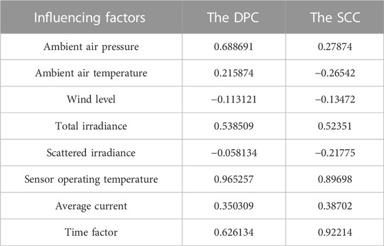
TABLE 3. The results of the through-hole analysis.
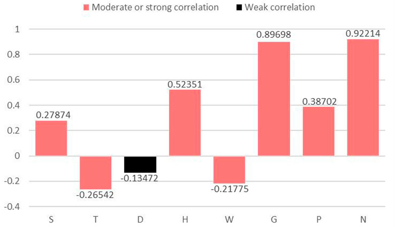
FIGURE 4. The SCC of influencing factors bar chart.
As can be seen from Figure 4, PV power is positively correlated (Bar facing up) with S, H, G, P, and N, and negatively correlated (Bar facing down) with T, D, and W. Meanwhile, the SCC definition indicates (Hu et al., 2018) that when its absolute value is at least 0.2, the correlation is moderate or strong (The bars are red). When the absolute value of the SCC is less than 0.2, the correlation is weak or there is no correlation (The bars are black). Therefore, we take the absolute value of the SCC 0.2 as the threshold value and select S, T, H, W, G, P, and N (ambient air pressure, ambient air temperature, total irradiance, scattered irradiance, sensor operating temperature, average current, and time factor) together as the seven primary influencing factors for distributed PV power prediction.
The SCC is used not only to screen the main influencing factors, but also to participate in the screening of similar time periods. The network parameters of the prediction model are first initialized and the optimal parameters of the corresponding method are obtained after the end of the cycle. The limit values (GM) of the CIC and the SCC are respectively set to 0.87 and 0.8. The minimum number (NM) of similar time periods are respectively taken to be 4 and 7. This is shown in Table 4.
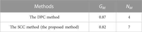
TABLE 4. The optimal parameters.
The number of similar time periods can be varied from 4 to 90 based on the DPC and from 7 to 30 based on the SCC. This is because the proposed method can adjust the number of similar time periods according to the difference in the correlation values of each historical time period, so as to achieve the dynamic optimization of similar time periods.
To further demonstrate the effectiveness of the SCC to determine the similar time period screening criteria, the SCC and the DPC are respectively used as the weights of TOPSIS for PV power prediction, and the prediction results are compared with the traditional TOPSIS. Figure 5 shows the comparison of the prediction results based on the three weight coefficients and the prediction errors are shown in Table 5.
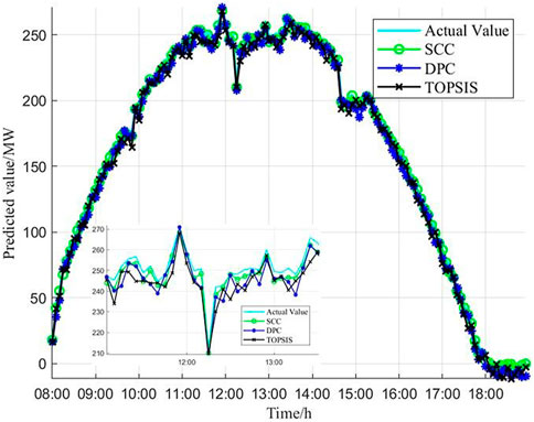
FIGURE 5. Simulation comparison of PV power prediction results by three coefficients.
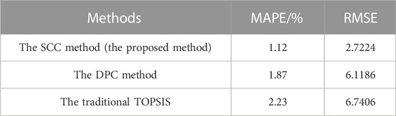
TABLE 5. Prediction errors of the three coefficient methods.
As shown in Figure 5, the prediction model curves of the direct path coefficient method and the traditional TOPSIS have obvious deviations at fluctuating time periods, such as the predicted values at 10:00–11:00, 12:00–13:00 and other time periods are lower than the true values. The introduction of the SCC for measuring the weight of each influencing factor solves the shortcomings of the traditional TOPSIS which generally selects 0.5 as the weight value, and makes the determination of the screening criteria more relevant. Therefore, the predicted curves fit better with the real curves after optimizing the traditional TOPSIS by the SCC.
As shown in Table 5, the average absolute percentage deviations of the predictions based on the SCC and the DPC are 1.12% and 1.87%, respectively, both of which are less than 2%, while the value of this error for the traditional TOPSIS is 2.23%, indicating that the weight parameters of TOPSIS are effectively optimized by using both coefficients obtained from path analysis.
Meanwhile, the predicted PV power curves of the three methods are roughly similar to the trend of the actual curve to be predicted, which verifies the validity of the ISTP selection results.
5.3 PV power short-term prediction results
To verify the effectiveness and superiority of the ISTP model, the traditional similar day (Ding et al., 2012) method and the ELMAN neural network (Ye et al., 2017) are applied to predict PV power for the same days and compared with the proposed method. The comparison results of prediction curves and errors of the three models are shown in Figure 6 and Figure 7: (a) ISTP (b) similar day (c) the ELMAN neural network. Table 6 indicates specific values of errors for the three models, respectively.
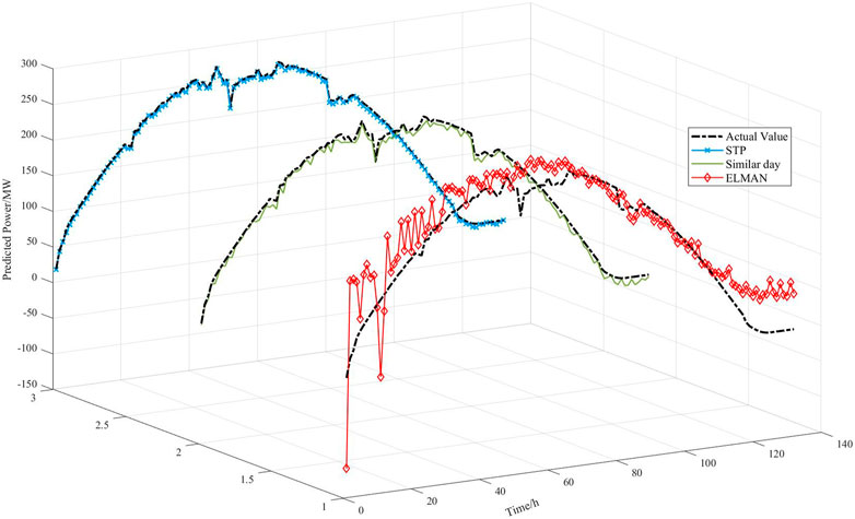
FIGURE 6. Simulation comparison of PV power prediction results by three models.
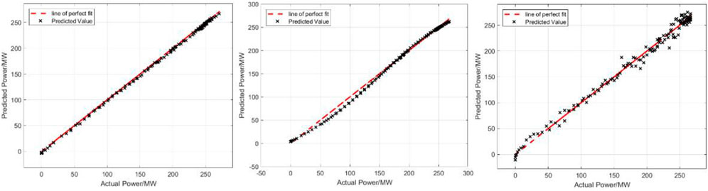
FIGURE 7. Comparison of the errors by three models.
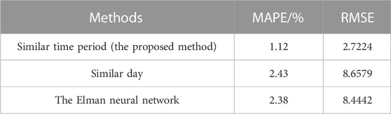
TABLE 6. Prediction errors of the three models.
As can be seen from Figure 6, because similar day method is analyzed purely from the perspective of power values, the screening criteria are single and it is difficult to avoid the overall bias. Except for the 11:00–14:00 time period which has higher fluctuations, the prediction curve shows an overall trend of larger predicted values than the actual values. The ELAMN neural network is affected by the model’s characteristics. Even in the period when the actual curve is relatively smooth, there are still large fluctuations in the prediction curve and the fluctuations are most obvious in the larger part of the power value, such as poor data matching in the period from 10:00 to 16:00. The proposed ISTP method introduces the CIC as screening criteria and dynamically optimizes the number of similar time periods.
At the same time, the errors of models based on similar day method and the ELMAN neural network method are 2.43% and 2.38%, respectively, which are both greater than 2%. In contrast, the error of the proposed method is less than 2%, which is only 1.12%. The comparison of the prediction error evaluation criteria intuitively reflects that after the introduction of TOPSIS optimized by the SCC and the CIC, PV power prediction model established by the proposed method is closer to the actual model and has a greater improvement effect on the prediction accuracy.
6 Conclusion
We propose a method for short-term prediction of distributed PV power by improving similar time period method. Our method can effectively ensure a strong correlation between the similar periods and the periods to be predicted. First, it is proposed to determine the SCC based on path analysis and then set a threshold to select main influencing factors, which can effectively eliminate redundant information, reduce data dimensionality, and simplify model building. Second, the screening criteria of the CIC are proposed, which can dynamically optimize the number of similar time periods for each time period to be measured and obtain the optimal prediction results. Finally, the proposed modeling method effectively reduces the amount of data and the algorithm training is simple and more conducive to programming implementation, which has engineering application value. Experimental results demonstrate that MAPE% of proposed ISTP method are, respectively, improved by 47.06% and 46.09% compared with the traditional ELMAN and similar day method.
However, the sample capacity of similar periods during sudden weather is small, and the mean value is used to supplement the number of similar periods in the paper, which could possibly lead to a decrease in prediction accuracy.
Future studies will cluster the weather and try to expand sample capacity with intelligent algorithms when the number of similar periods in sudden weather is small, so as to lay the foundation for regional prediction.
Data availability statement
The original contributions presented in the study are included in the article/supplementary material, further inquiries can be directed to the corresponding author.
Author contributions
YZ is the corresponding author and takes primary responsibility. ZW contributed for the analysis of the work and wrote the first draft of the manuscript. All authors contributed to the manuscript revision, and read and approved the submitted version.
Conflict of interest
The authors declare that the research was conducted in the absence of any commercial or financial relationships that could be construed as a potential conflict of interest.
Publisher’s note
All claims expressed in this article are solely those of the authors and do not necessarily represent those of their affiliated organizations, or those of the publisher, the editors and the reviewers. Any product that may be evaluated in this article, or claim that may be made by its manufacturer, is not guaranteed or endorsed by the publisher.
References
Antonanzas, J., Osorio, N., Escobar, R., Urraca, R., Martinez-de-pison, F. J., and Antonanzas-Torres, F. (2016). Review of photovoltaic power forecasting. Sol. Energy 136, 78–111. doi:10.1016/j.solener.2016.06.069
Chen, T., Sun, G., Wei, Z., Zang, H., Sun, Y., et al. (2017). Photovoltaic power generation forecasting based on similar day and CA-PSO-SNN. Electr. Power Autom. Equip. 37 (3), 66–71. doi:10.16081/j.issn.1006-6047.2017.03.012
Cheng, Z., Liu, C., and Liu, L. (2017). A method of probabilistic distribution estimation of PV generation based on similar timeof day. Power Syst. Technol. 41 (2), 448–454. doi:10.13335/j.1000-3673.pst.20
Ding, M., Wang, L., and Bi, Y. (2012). A short-term prediction model to forecast output power of photovoltaic system based on improved BP neural network. Power Syst. Prot. Control 40 (11), 93148–93199. doi:10.3969/j.issn.1674-3415.2012.11.016
Fu, M. P., Ma, H. W., and Mao, J. R. (2012). Short-term photovoltaic power forecasting based on similar days and least square support Vector machine. Power Syst. Prot. Control 40 (16), 65–69. doi:10.3969/j.issn.1674-3415.2012.16.011
Ge, L. J., Qin, Y. F., Liu, J. H., and Bai, X. Z. (2021). Virtual acquisition method of distributed photovoltaic data based on similarity day and BA-WNN. Electr. Power Autom. Equip. 41 (6), 8–14. doi:10.16081/j.epae.202106011
Hu, C., Zhang, Z., Jiao, Y., Li, H. B., and Chen, G. (2018). Error state correlation analysis based on random matrix theory for electronic transformer. Electr. Power Autom. Equip. 38 (9), 45–53. doi:10.16081/j.issn.1006-6047.2018.09.008
Kıvanç, B., Fatma, B., Pierluigi, S., Pelin, Y. T., and Deniz, K. (2020). Systematic literature review of photovoltaic output power forecasting. IET Renew. Power Gener. 14 (19), 3961–3973. doi:10.1049/iet-rpg.2020.0351
Li, J. W., Jiao, H., Liu, F. W., and Wang, X. Y. (2018). Short-time segmented photovoltaic output forecasting based on similar period. Electr. Power Autom. Equip. 38 (8), 183–188. doi:10.16081/j.issn.1006-6047.2018.08.026
Lu, Z. X., Wang, B., and Rong, J. F. (2017). Photovoltaic generation power prediction based on multi-period integrated similar days. Chin. J. Power Sources 41 (1), 103–106. doi:10.3969/j.issn.1002-087X.2017.01.033
Luo, P., Zhu, S., Han, L., and Chen, Q. (2018). “Short-term photovoltaic generation forecasting based on similar day selection and extreme learning machine,” in 2017 IEEE Power & Energy Society General Meeting (IEEE). doi:10.1109/PESGM.2017.8273776
Niu, D. X., Wang, K. K., Sun, L. J., Wu, J., and Xu, X. M. (2020). Short-term photovoltaic power generation forecasting based on random forest feature selection and ceemd: A case study. Appl. Soft Comput. 93, 106389. doi:10.1016/j.asoc.2020.106389
Peng, W., Xie, F. Y., and Zhang, Z. Y. (2019). Short-term wind power forecasting algorithm based on similar time periods clustering. Proc. CSU-EPSA 31 (10), 81–87. doi:10.19635/j.cnki.csu-epsa.000167
Qiao, Y., Sun, R. F., Ding, R., Li, S. Q., and Lu, Z. X. (2021). Distributed photovoltaic station cluster gridding short-term power forecasting part I: Methodology and data augmentation. Power Syst. Technol. 45 (5), 1799–1808. doi:10.13335/j.1000-3673.pst.2021.0305
Sheng, W., Wu, M., Ji, Y., Kou, L., Pan, J., et al. (2019). Key technologies and engineering practice of distributed renewable energy power generation cluster integration and consumption. Proc. CSEE 39 (8), 2175–2186. doi:10.13334/j.0258-8013.pcsee.182456
Sun, Q., Yao, J. G., Zhao, J., Jin, M., Mao, L. F., et al. (2013). Short-term bus load integrated forecasting based on selecting optimal intersection similar days. Proc. CSEE 33 (4), 126–134.
Tan, F. L., Chen, H., and He, J. H. (2021). Top oil temperature forecasting of UHV transformer based on path analysis and similar time. Electr. Power Autom. Equip. 41 (11), 217–224. doi:10.16081/j.epae.202109026
Utpal, K. D., Kok, S. T., Mehdi, S., Saad, M., Moh, Y. I. I., Van Deventer, W., et al. (2018). Forecasting of photovoltaic power generation and model optimization: A review. Renew. Sustain. Energy Rev. 81 (1), 912–928. doi:10.1016/j.rser.2017.08.017
Wang, X. L., and Ge, P. J. (2013). PV array output power forecasting based on similar day and RBFNN. Electr. Power Autom. Equip. 33 (1), 100–103. doi:10.3969/j.issn.1006-6047.2013.01.019
Wu, C., Dong, A., Li, Z., and Wang, Fei. (2022). PV power prediction based on graph similarity day and PSO-XGBoost. High. Volt. Technol. 48 (08), 3250–3259. doi:10.13336/j.1003-6520.hve.20211815
Ye, R. L., Guo, Z. Z., Liu, R. Y., and Liu, J. N. (2017). Wind speed and wind power forecasting method based on wavelet packet decomposition and improved Elman neural network. Trans. China Electrotech. Soc. 32 (21), 103–111. doi:10.19595/j.cnki.1000-6753.tces.160727
Zhang, J., Verschae, R., Nobuhara, S., and Lalonde, J. F. (2018). Deep photovoltaic nowcasting. Elsevier Science. doi:10.1016/j.solener.2018.10.024
Zhang, L. H., Zang, M., Ji, W. L., Fang, L., Qin, Y. F., et al. (2021). Virtual acquisition method for operation data of distributed PV applying the mixture of grey relational theory and BP. Electr. Power Constr. 42 (1), 125–131. doi:10.12204/j.issn.1000-7229.2021.01.014
Zhao, B., Guo, C. X., Zhang, P. X., and Cao, Y. J. (2005). Distributed cooperative parti⁃ swarm optimization algorithm for reactive power opti⁃ mization of power systems. Chin. J. Electr. Eng. Proc. CSEE) 25 (21), 1–7. doi:10.3321/j.issn:0258-8013.2005.21.001
Keywords: distributed photovoltaic power plant, path analysis, TOPSIS, PV power prediction, improved similar period
Citation: Wu Z, Zhang Y, Liu B and Zhang M (2023) Short-term prediction for distributed photovoltaic power based on improved similar time period. Front. Energy Res. 11:1149505. doi: 10.3389/fenrg.2023.1149505
Received: 22 January 2023; Accepted: 13 February 2023;
Published: 23 February 2023.
Edited by:
Kada Bouchouicha, CDER, AlgeriaReviewed by:
Nadjem Bailek, Université Ahmed Draia Adrar, AlgeriaBellaoui Mebrouk, Centre de Développement des Energies Renouvelables, Algeria
Copyright © 2023 Wu, Zhang, Liu and Zhang. This is an open-access article distributed under the terms of the Creative Commons Attribution License (CC BY). The use, distribution or reproduction in other forums is permitted, provided the original author(s) and the copyright owner(s) are credited and that the original publication in this journal is cited, in accordance with accepted academic practice. No use, distribution or reproduction is permitted which does not comply with these terms.
*Correspondence: Yi Zhang, emhhbmd5aUBmenUuZWR1LmNu