Techno-economic optimal planning of an industrial microgrid considering integrated energy resources

Microgrids have benefited energy systems by getting rid of the abundant use of traditional energy resources, replacing them with distributed generations (DGs). The use of DGs in microgrids not only provides clean and green energy but also reduces the gigantic losses in transmission and distribution lines. Widespread adoption of renewable energy in microgrids saves customers from high fuel prices and provides a sustainable replacement for future fossil fuel depletion. Microgrids have proven to be the latest and most advanced power systems due to their new capabilities to operate in both grid-connected and isolated modes. Microgrids use multiple energy sources simultaneously, which can offset the intermittent behavior of renewable energy sources. In this study, we planned and optimized an industrial microgrid with an annual increase in load, which contains dispatchable generation, non-dispatched generation, and energy storage. In addition, to test the different behavior of a microgrid operating independently or in grid-tied mode, four typical days were selected to show the load demand and solar and wind energy forecast data for the entire year. The power output curves for each typical day were analyzed for every year in both stand-alone and grid-connected modes. Furthermore, to validate the feasibility of the microgrid, the investment and operations costs were also calculated in the paper.

1 Introduction

Global warming and climate change are wreaking havoc in the world in the form of torrential rains, floods, and other natural calamities. In order to reduce carbon footprint and global warming, the world has vowed to focus on clean and green energy through robust and state-of-the-art technologies. Smart grids, distributed generations (DGs), and sustainable energy policies can play a substantial role in reducing the increasing load demand and carbon emission impact on human lives. To fully achieve the maximum benefits of DGs, it is important to reassess the cornerstone assumptions underlying the powers systems (PSs). In the recent decade, DG has evolved as a cost-effective and environmentally sustainable alternative to conventional electric energy sources, and technological innovations are enabling DGs to be economically viable (Ackermann et al., 2001). The most interesting characteristic of DG is that it is scattered throughout the network, is nearby to customers, offers several different technologies, and provides massive energy (Ali et al., 2023). There are various resources about DG technology and integration. Researchers need to comprehend the problematic situation of DGs in the power system (Wu et al., 2020). There is no specific definition of DG yet owing to developing technology and the increasing scale, which play an essential and fascinating role in the advancement of a power system. DGs are also known as embedded generations or scattered generations (Zoka et al., 2004). Some of the popular DG technologies include reciprocating diesel or natural gas engines (Malik et al., 2021), micro-turbines or hydropower (Asano and Bando, 2006), combustion gas turbines (Peterman, 1988), fuel cells (Ali et al., 2022), photovoltaic (PV) systems (Hadjsaid et al., 1999), and wind turbines (Nfah and Ngundam, 2008). Figure 1 provides a vivid overview of the frequently used DG technologies (Weis and Ilinca, 2008). Hydro, wind, PV, geothermal, and ocean energy can be considered renewable DGs. Other technologies that run on bio-fuels could also be classified as renewable DGs. Similar to centralized generation, DG often involves the following three generating technologies: synchronous generator, asynchronous generator, and power electronic converter interface (Laghari et al., 2013). A comprehensive study by the Department of Energy Laboratory (NREL) shows that the U.S. will generate 80% of its electric power from renewable energy by 2050 (Vallem and Mitra, 2005). The microgrid, as defined by the U.S. Department of Energy, is “a group of interconnected loads and distributed energy resources (DERs) with clearly defined electrical boundaries that acts as a single controllable entity with respect to the grid and can connect and disconnect from the grid to enable it to operate in both grid-connected or island modes” (National Renewable Energy Laboratory, 2021).

FIGURE 1

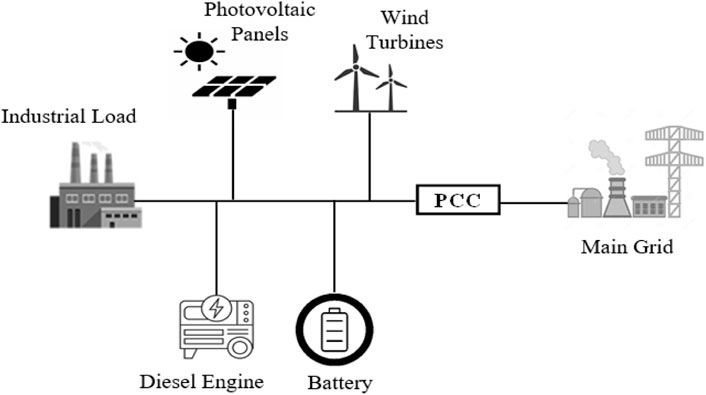
FIGURE 1. Typical microgrid connected to the utility grid for industrial microgrid planning.

The microgrid consists of loads, DERs, a master controller, smart switches, protective devices, and communication, control, and automation systems. Microgrid loads are generally characterized into two types: fixed loads and flexible loads (which are also known as adjustable or responsive loads) (Ton and Smith, 2012). Microgrid generation is classified as either dispatchable or non-dispatchable. Non-dispatchable units, on the other hand, cannot be controlled by the microgrid master controller because the input source is uncontrollable (Rehman et al., 2017). Dispatchable units, on the contrary, are subject to technological limitations depending on the type of unit, such as capacity limits, ramping limits, minimum on/off time limits, and fuel and emission limits. Renewable DGs, such as solar and wind DGs, are non-dispatchable because their output power is volatile and intermittent (Duffy et al., 2018).

The intermittency factor indicates that the generation is not always available, whereas the volatility factor implies that the generation varies over time. Because these properties have an unfavorable influence on the non-dispatchable unit generation and huge forecast inaccuracy, these units are frequently re-enforced with energy storage systems (ESSs) (Hirsch et al., 2018). The major function of the ESS is to synchronize with DGs to provide adequate microgrid generation. Such systems can also be utilized for energy trade, in which the stored energy is generated and supplied to the microgrid when market prices are high. In microgrid islanding applications, the role of the ESS is highly significant (Dutta et al., 2021). By connecting and disconnecting line flows, smart switches and protective devices regulate the connection between DERs and loads in the microgrid. When a microgrid link fails, smart switches and protective devices remove the affected and faculty areas and re-route electricity by preventing the fault from escalating throughout the microgrid (Tao et al., 2010). By isolating the microgrid from the utility grid, the switch at the point of common coupling (PCC) achieves microgrid islanding. The microgrid master controller manages microgrids in interconnected and islanded modes based on economic and safety issues. The microgrid interface with the utility grid (UG), the decision to switch between interconnected and islanded modes, and the optimal operation of local resources are all controlled by the master controller. To carry out these control actions and ensure continuous, effective, and reliable connection among microgrid elements, communications, control, and automation systems are also used (Yona et al., 2007).

The islanding capability is the most outstanding feature of a microgrid, which is enabled by employing switches at the PCC and permits the microgrid to be disconnected from the utility grid in case of utility grid disturbances or voltage variations (Habib et al., 2022). During upstream disturbances, the microgrid is shifted from the grid-connected mode to the islanded mode, and a reliable and uninterrupted supply of consumer loads is offered by local DERs. The islanded microgrid would be resynchronized with the utility grid as soon as the disturbance is removed (Shuaixun, 2012). KSA has committed to installing 27.3 GW of renewable energy (RE) by 2023, the majority of which (20 GW) will be generated from PV panels, while the remaining 7.3 GW will be generated from wind energy and concentrated solar power (CSP). By the end of 2030, a total of 40, 16, and 2.7 GW will be generated from solar PV, wind, and CSP energy, respectively (Zhou et al., 2019). The road maps show how 80 to 85 percent of existing energy could be replaced by wind, water, and solar energy by 2030, with 100 percent by 2050 in the USA (Li et al., 2017). The main contributions of the paper are as follows:

• This paper presents optimal planning of an industrial microgrid which comprises diesel engines, PV panels, wind turbines, and ESSs in stand-alone and grid-connected modes for a period of 5 years.

• The investment and O&M costs of the microgrid are calculated in this paper to show the feasibility of the model. It also considers the typical days to validate the load demand variations, seasonal changes, intermittency, and volatility of the RES.

2 Microgrid planning model

2.1 PV model

In the PV system, the maximum power point tracker (MPPT) is selected and used. The maximum power output ($P_s$) is obtained by Eq. 1 (Iniyan et al., 1998; Maulik and Das, 2017; Abbas et al., 2022), where η is the conversion efficiency of the solar cell array (%), $A_{pv}$ is the array area (m²), $G_T$ is the solar radiation (kW/m²), and $T_0$ is the outside air temperature (°C). Figure 2 shows the voltage and current characteristic curves of a photovoltaic (PV) cell.

$P_s=\eta A_{pv}{G}_T\left[1-0.005\left(T_0-25\right)\right].(1)$

FIGURE 2

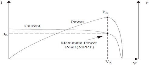
FIGURE 2. V–I characteristic curve and maximum power point of PV (Dutta et al., 2021).

2.2 Wind model

A piecewise function can be simply employed to fit the relationship between output power $P_r$ and wind speed ($v$), which is shown in Figure 3A (Yona et al., 2007). The mathematical expressions for obtaining wind power ($P_w$) are presented in Eq. 2. A plot of $P_w$ versus v based on Eq. 2 is presented in Figure 3B (Habib et al., 2022).

$P_w=\left\{\begin{array}{l}0,v\le v_c\\ {\mathrm{P}}_r.\frac{v-v_i}{v_r-v_i},v_c\le \mathrm{v}\le {\mathrm{v}}_f\\ P_r,v_r\le v\le v_f\\ 0,v\ge v_f\end{array}\right.(2)$

where $P_r$ is the rated power of the wind turbine, $v$ is the wind speed, $v_c$ is the cut-in wind speed, $v_r$ is the rated wind speed, and $v_f$ is the cut-out speed.

FIGURE 3

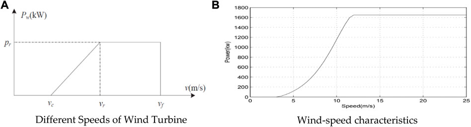
FIGURE 3. Different parameters of wind turbines for the analysis of their power and speed generation. (A) The curve of different speeds of wind turbines (Yona et al., 2007). (B) Waveform showing the wind speed characteristics (Habib et al., 2022).

In Figure 3B, the cut-in wind speed $v_c$ is the minimum speed to start the WTs, and the cut-out wind speed $v_f$ is the maximum speed to shut down the WTs. Some error exists between the calculated wind power and the real wind power due to the error in the forecasted wind speed. The error is expressed as a root mean square error (RMSE) for the time-series model. The actual power obtained from the wind turbines is given by the following equation (Shuaixun, 2012):

$P=P_w{A}_w\eta .(3)$

In Eq. 3, $A_w$ is the total swept area and η is the efficiency of the wind turbine generator and corresponding converters.

2.3 Battery model

The lifetime of the battery is given in n years, and its maintenance cost is given by $M{C}_B=\left(n\times MC\right)$, i.e., $/kWh per year, and the total cost of the battery is calculated as $Total=In{v}_B+M{C}_B$. However, in this model, only the investment cost $In{v}_B$ is considered, which is given in Eq. 4, while the annual maintenance cost $M{C}_B$ is neglected.

$In{v}_B=CRF\times \left(C{E}_{n,B}^{inv}\cdot C_B^{rated}+C{P}_{n,B}^{inv}\cdot CP\right).(4)$

2.4 Diesel engine model

The investment cost of the diesel generating unit ($C_{Diesel}^{Inv}$) is a function of its generating capacity which is expressed as follows:

$C_{Diesel}^{Inv}=C_{n,Die}^{Inv}\cdot P_{Die}^{rated}.(5)$

The output power constraint of the diesel engine model is given as

$0\le P_{n,d,h,Die}^{out}\le P_{Die}^{rated}.(6)$

3 Optimization model of an industrial microgrid

3.1 Objective function

Perceiving from the angle of a social planner, the investment cost related to diesel engines, photovoltaics, wind generation, and batteries are considered in the domain of the objective function. The terse expression of the objective function is depicted as

${\mathit{min}\mathrm{C}\mathrm{o}\mathrm{s}\mathrm{t}=\mathrm{C}}^I+C^{OM},(7)$

where $C^I$ and $C^{OM}$ represent the investment cost and operation and maintenance costs, respectively. The planning for the microgrid is simulated for 5 years. To validate the variability, four typical days are chosen for each year.

3.1.1 Investment cost ($IC$)

The investment cost ($IC$) of the planned industrial microgrid can be calculated as follows:

$IC={\displaystyle \sum }_{n=1}^{N}CRF\times DC\times \left(C_{n,Die}^{Inv}\cdot P_{Die}^{rated}+C_{n,PV}^{Inv}\cdot P_{PV}^{rated}+C_{n,WT}^{Inv}\cdot P_{WT}^{rated}+C{E}_{n,B}^{Inv}\cdot C_B^{rated}+C{P}_{n,B}^{Inv}\cdot P_{Die}^{rated}\right).(8)$

In Eq. 8, $C_{n,Die}^{Inv}$, $C_{n,PV}^{Inv}$, $C_{n,WT}^{Inv}$, $C{E}_{n,B}^{Inv}$, and $C{P}_{n,B}^{Inv}$ are the capital costs of the diesel engine, PVs, WTs, and battery used in the microgrid model, respectively. $P_{Die}^{rated}$, $P_{PV}^{rated}$, $P_{WT}^{rated}$, $C_B^{rated}$, and $P_{Die}^{rated}$ are the rated power of the diesel engine, PVs, WTs, and power and energy capacity of the battery, respectively.

The capital recovery factor ($CRF$) can be calculated using

$CRF=\left(\frac{d{\left(1+d\right)}^n}{{\left(1+d\right)}^n-1}\right).(9)$

The discount cost ($DC$) is obtained using the mathematical expression given as follows:

$DC=\left(\frac{1}{{\left(1+d\right)}^n}\right).(10)$

In Eqs 9, 10, d is the interest rate and n is number of years for which planning is carried out.

3.1.2 Operational and maintenance costs ($C^{OM}$)

$C^{OM}={\displaystyle \sum }_{n=1}^N{\displaystyle \sum }_{d=1}^N{\displaystyle \sum }_{h=1}^{N}DC\times \left(C_{Die}\cdot P_{n,d,h,Die}^{out}+C_{Pv}\cdot P_{n,d,h,PV}^{out}+C_{WT}\cdot P_{n,d,h,WT}^{out}+C_{buy}\cdot P_{n,d,h}^{buy}\right).(11)$

In Eq. 11, N is the planning horizon; $C^{OM}$ represents the microgrid operational and maintenance costs, including the unit commitment cost, fuel cost, and unit operation cost; $C_{Die}$ is the fuel cost of a diesel engine; $P_{n,d,h,Die}^{out}$ is the output power of a diesel engine at h hour, d days, and n years; $C_{PV}$ is the operational and maintenance cost of the PV unit; $P_{n,d,h,PV}^{out}$ is the output power of the PV unit at h hour, d days, and n years; $C_{WT}$ is the operational and maintenance cost of the WPP unit, $P_{n,d,h,WT}^{out}$ is the output power of the WPP unit at h hour, d days, and n years; $C_{buy}$ is the power purchasing cost of a microgrid (MG) from the main grid; $P_{n,d,h}^{Buy}$ is the power bought from the UG at h hour, d days, and n years; and DC is the discount cost.

3.2 Constraints

The constraints to the objective function of the proposed optimization model are expressed separately.

3.2.1 Power balance constraint

When the generation capacity of the system is unable to meet the energy demand at some specific hours, the MG requires power to be transported from the UG or battery to avoid a blackout. The power balance of the system is expressed as

$P_{n,d,h,Die}^{out}+P_{n,d,h,PV}^{out}+P_{n,d,h,WT}^{out}-P_{n,d,h}^{Ch}+P_{n,d,h}^{DisCh}+P_{n,d,h}^{Buy}={\left(1+\theta \right)}^{n-1}{P}_{b,d,h,D}.(12)$

In Eq. 12, $P_{n,d,h,Die}^{out}$ represents the output power of a diesel engine at h hour, d days, and n years; $P_{n,d,h,PV}^{out}$ represents the output power of PV units at h hour, d days, and n years; $P_{n,d,h,WT}^{out}$ represents the output power of wind turbines unit at h hour, d days, and n years; $P_{n,d,h}^{Ch}$ is the ESS power charging at h hour, d days, and n years; $P_{n,h}^{DisCh}$ is the ESS power discharging at h hour, d days, and n years; $P_{n,d,h}^{Buy}$ is the power bought from the main gird at h hour, d days, and n years, $\theta$ is the load growth rate; and $P_{n,d,h,D}$ is the demand forecast at h hour, d days, and n years.

3.2.2 Diesel engine constraints

The output power constraints of the diesel engine are expressed as

$0\le P_{n,d.h,Die}^{out}\le P_{Die}^{rated}.(13)$

3.2.3 Photovoltaic constraints

The output power constraints of the photovoltaic panels are expressed as

$0\le P_{n,d.h,PV}^{out}\le Coef{f}_{d,h}\times P_{PV}^{rated}.(14)$

3.2.4 Wind turbine constraints

The output power constraints of the wind turbines are expressed as

$0\le P_{n,d.h,WT}^{out}\le Coef{f}_{d,h}\times P_{WT}^{rated}.(15)$

3.2.5 Power buying constraints

To meet the power deficiency of the MG, its power buying constraints are given as

$0\le P_{n,d.h}^{buy}\le P_{\max }^{buy}.(16)$

3.2.6 Battery charging constraints

The constraints for charging a battery are expressed as

$0\le P_{n,d.h}^{ch}\le P_B^{rated}.(17)$

3.2.7 Battery discharging constraints

The constraints to discharge a battery are expressed as

$0\le P_{n,d.h}^{Disch}\le P_B^{rated}.(18)$

3.2.8 Battery energy storage constraints

A battery can store a certain amount of energy. The energy storage constraints of a battery are expressed as

$0\le E_{n,d,h}\le C{B}_B^{rated}.(19)$

It should be noted that in the first hour of the battery, the energy of the battery will be stored according to the following equation:

$E_{d,1}=\left(0.5\times C_B^{rated}+P_{d,h}^{ch}\times {\eta }_{ch}-P_{d,h}^{DisCh}/{\eta }_{DisCh}\right).(20)$

The energy storage in the battery after the first hour will be according to the following equation:

$E_{d,h}=\left(E_{d,h-1}+P_{d,h}^{Ch}\times {\eta }_{ch}-P_{d,h}^{DisCh}/{\eta }_{ch}\right)\mathrm{h}=2\dots 24\mathrm{w}\mathrm{h}\mathrm{e}\mathrm{r}\mathrm{e}\mathrm{h}=2\dots 24.(21)$

It is worth noting that at the last hour of the battery, energy in the battery will be half of its capacity as shown in the following equation:

$E_{d,24}=0.5\times C_B^{rated}.(22)$

4 Case study

4.1 Settings for the industrial microgrid

In this study, we modeled an industrial microgrid to meet the electrical load demand. It comprises two non-dispatchable units, i.e., WTs and PV panels, battery storage, and five different capacity dispatchable units, i.e., the diesel generators, as given in Table 1, Table 2, and Table 3, respectively. The efficiency of the battery storage is to be considered 90%. The load demand data for four typical days are selected in order to validate the whole year data, while 12% load growth is also considered for each planned year. The graphs for the selected data of four typical days for the forecasted load demand, solar power, and wind power are vividly expressed in Figure 4, Figure 5, and Figure 6, respectively. The power purchasing and selling costs to/from the UG are given in Table 4. The planning horizon for the industrial microgrid is kept for 5 years, and the discount rate chosen for the said planning is 5%.

TABLE 1

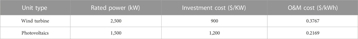
TABLE 1. Parameters of the non-dispatchable generators for the industrial microgrid (Du et al., 2020).

TABLE 2

TABLE 2. Parameters of energy storage devices for the industrial microgrid (Du et al., 2020).

TABLE 3

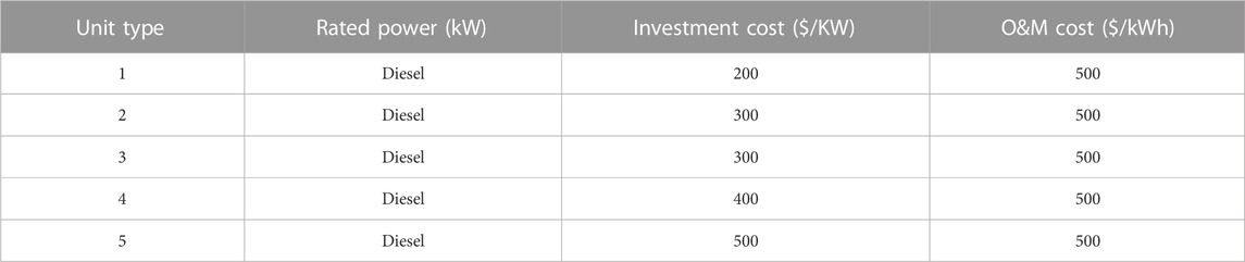
TABLE 3. Parameters of dispatchable generators for the industrial microgrid (Yona et al., 2007).

FIGURE 4

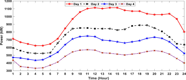
FIGURE 4. Typical 4-day forecasted load demand for the industrial microgrid (Cardenas et al., 2022).

FIGURE 5

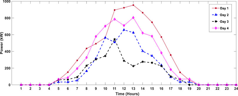
FIGURE 5. Typical 4-day forecasted PV power for the industrial microgrid (Khezri et al., 2021).

FIGURE 6

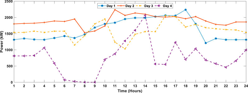
FIGURE 6. Typical 4-day forecasted wind power for the industrial microgrid (Khezri et al., 2021).

TABLE 4

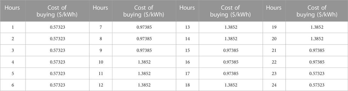
TABLE 4. Cost of buying power for the industrial microgrid from the main grid (Yona et al., 2007).

To carry out the planning and optimization of the industrial microgrid, a personal computer—Intel(R) Core (TM) i5-5200U CPU at 2.20 GHz with Windows 8.1 64-bit—was used, and the code was formulated in MATLAB software. The commercial solver CPLEX was chosen for solving the code and finding optimal results of the planned microgrid.

The different typical forecasted load demand curves for 4 days are given in Figure 4. It is evident from Figure 4 that the second day has the lowest load demand as compared to the other days and the maximum load demand is presented on the fourth day as compared to the other three typical days, whereas the third day and first day have the average load demand as compared to the other 2 days.

The forecasted PV power curves for the selected four typical days are given in Figure 5. It is noticed in Figure 5 that the highest power curve is given on the first day, and the lowest power curve is on the third typical day. It means that the maximum power is generated by the PV panels on the first typical day, and in contrast, the minimum power is generated on the third typical day. The power curve on the second and fourth typical days are on average as compared to the power curves of the first and third typical days. Due to the intermittent behavior of solar irradiance, the power on each day might change; hence, the typical days are chosen to validate the intermittency of the solar irradiance.

The forecasted wind power curves for the four chosen typical days are given in Figure 6. It is evident from Figure 6 that wind power curves are more zig-zag because the power produced in WTs fluctuates due to the volatility of the wind speed. From Figure 6, it is noted that the maximum power is generated on the second day and the minimum power is generated on the first day, as compared to the other two typical days, which both lie between the maximum and minimum power generation.

4.2 Multi-year planning results of the isolated industrial microgrid

The results for the planned isolated industrial microgrid are presented in Table 5. It can be noticed that in the first year, a capacity of 916 kW PV, 1,292 kW wind, 200 kW diesel engine, and 288 kW battery is planned, which results in a total capacity of 2,697 kW. In the second year, the load demand jumps by 12%, which is more than the first year, and an increase of 61 kW only is needed in a diesel engine to meet the load demand of the second year as compared to the previous year. In the third year, the load growth coefficient is 1.25 more than in the second year, so more capacity is required to meet the load demand of the power system, that is, 1,500 kW PV, 2,400 kW wind, 300 kW diesel engine, and 308 kW battery, which becomes 4,508 kW in total for the third year. In the fourth year, as the load growth coefficient is 1.4, 4,585 kW capacity is needed to meet the load demand, in which there is a 77 kW increase in the diesel engine capacity as compared to the fourth year because all the other resources are already at their maximum rated power. In the fifth planned year, the load growth coefficient is 1.5, which results in more load demand than the fourth-year load demand, and in order to fulfill the fifth-year load demand, a capacity of 1,500 kW PV, 2,400 kW wind, 463 kW diesel engine, and 308 kW battery is planned.

TABLE 5

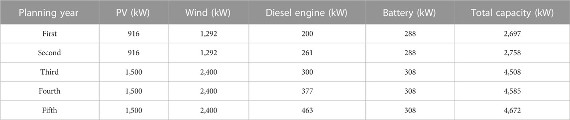
TABLE 5. Cost of buying power for the industrial microgrid from the main grid (Yona et al., 2007).

4.3 Multi-year planning results of the grid-connected industrial microgrid

The results for the planned grid-connected industrial microgrid are shown in Table 6. In the grid-connected mode, the main grid has the ability to buy power from the UG, and the limit to buy power is set at 300 kW. So, in grid-connected mode, the main grid in the first year needs 510 kW wind, 200 kW diesel engine, and 50 kW battery, which becomes a total capacity of 760 kW; however, it does not choose PV in the first year. In the second year, 725 kW wind, 300 kW diesel engine, and 80 kW battery amount to a total capacity of 1,106 kW to meet the load demand with a load growth coefficient of 1.2. In the third year, 955 kW wind, 300 kW diesel engine, and 119 kW battery result in 1,375 kW, which is planned to meet the load demand with a load growth of 1.25, and in this year also, PV is not chosen for a generation. In the fourth year, 115 kW PV, 1,018 kW wind, 400 kW diesel engine, and 119 kW battery amount to a total capacity of 1,653 kW, which meets the load demand with a load growth coefficient of 1.4 than the first-year load demand. However, in the fifth year, 524 kW PV, 1,095 kW wind, 500 kW diesel, and 246 kW battery are needed, which results in a total capacity of 2,366 kW to meet the load demand of the fifth year having a load growth factor of 1.5 than the first year. In grid-connected mode, along with these planned capacities, the left-over power is bought from the main grid, and their detailed depictions are shown in Figure 5, Figure 6, Figures 7A, B, Figures 8A, B, and Figures 9A, B, respectively.

TABLE 6

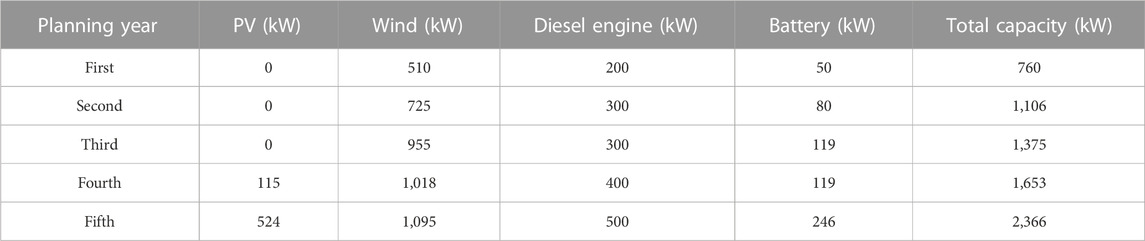
TABLE 6. Planning results for the grid-connected industrial microgrid.

FIGURE 7

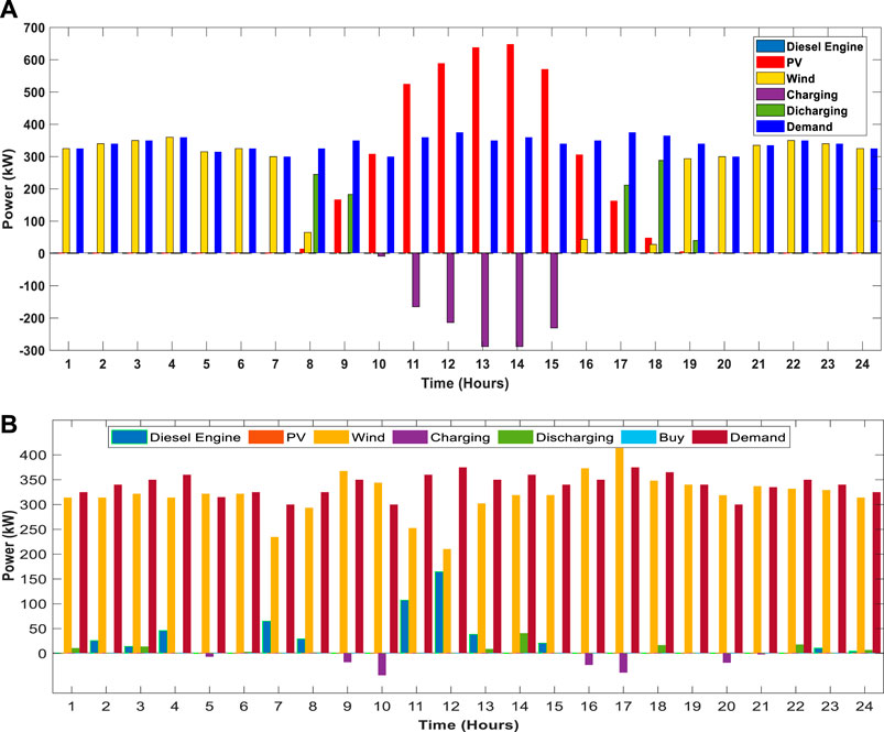
FIGURE 7. Power output curve meeting load demand on a typical day. (A) Stand-alone mode. (B) Grid-connected mode.

FIGURE 8

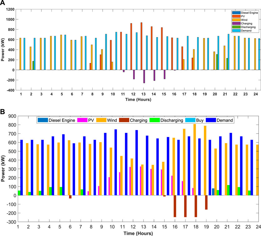
FIGURE 8. Power output curve meeting load demand on a typical day. (A) Stand-alone mode. (B) Grid-connected mode.

FIGURE 9

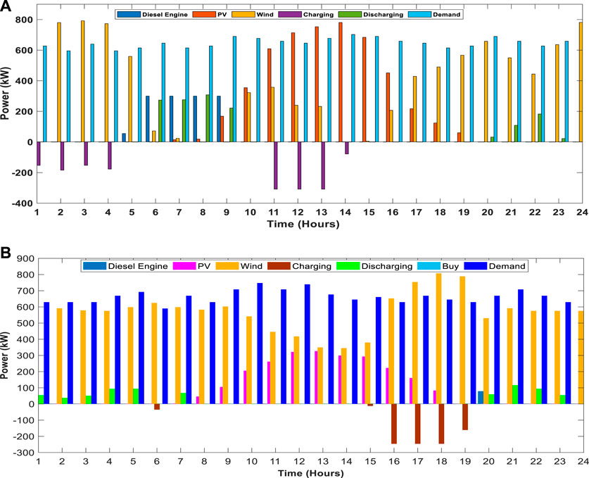
FIGURE 9. Power output curves to meet load demand on a typical day. (A) Stand-alone mode. (B) Grid-connected mode.

4.4 Output power curves of the industrial microgrid for typical days

In Figure 7A, the power output curves show that in the isolated mode, industrial MG PV, wind, and battery capacities are used to meet the load demand, while the diesel engine is not used to generate the power on the third typical day of the first year. Figure 7B shows that due to different capacity limits in the grid-connected mode, diesel engine, wind, and battery capacities are used to meet the load demand, and due to enough power availability within the main grid, no additional power is bought from the UG, and no PV capacity is utilized in the third typical day of the first year.

In Figure 8A, the power output curves show that wind, PV, and battery capacities are utilized to meet the load demand, while the diesel engine is not used to generate the power on the second typical day of the fourth year of industrial microgrid connected in the stand-alone mode. Figure 8B shows that due to the gargantuan capacity of PV and wind in the grid-connected mode, diesel engine and battery are not selected due to enough power availability from renewable energy sources (RES), so no further power is bought from UG in the second typical day of the fourth year to meet the load demand.

In Figure 9A, the power output curves show that PV, wind, and battery capacities are being utilized to meet the load demand, while the diesel engine is not used on the first typical day of the fifth year in the isolated mode of the industrial microgrid. Figure 9B shows that due to the grid-connected mode and the large capacity of PV, wind, and battery, only the power needed for 1 h is to be generated from the diesel engine to meet the load demand on the third typical day of the first year; it also noticed that on this typical day, the main grid does not buy power from the UG due to enough power availability from its resources.

4.5 The total investment and O&M costs of the industrial microgrid

The total planning cost for 5 years, which consists of investment and O&M costs of the industrial microgrid in both isolated and grid-connected modes, is given in Table 7.

TABLE 7

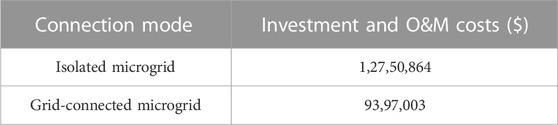
TABLE 7. Total investment and O&M costs of the industrial microgrid in both modes.

It can be noted from Table 7 that the total investment and O&M costs of the industrial microgrid in the grid-connected mode are much lower than in the isolated mode because in the grid-connected mode, it chooses to install power capacity lower than that of the isolated mode of the microgrid, and it is also an ability to buy power from the UG in case of power scarcity which mainly results in the reduction of the heavy investment and O&M costs.

5 Conclusion

In this paper, we planned an industrial microgrid considering multiple energy resources for 5 years. The main objective of the planning and optimization of the microgrid was to reduce the hefty investment and O&M costs of the planned industrial microgrid. In order to validate the model and several aspects of seasonal variations and the day–night behavior of PV, wind, and load demand, four typical days were selected for every planned year. Furthermore, to show the trend of the load growth for future needs and power system expansion, a load growth factor of 12% was kept for each year for the industrial microgrid. To justify the model further, several simulations were carried out on the model to obtain different power output results on both grid-connected and isolated modes of the simulated MG. The results depict that in the isolated mode, the microgrid requires more capacity of the distributed generation to meet the load demand because, and in the stand-alone mode, there is no connection to the external UG. However, in the grid-connected mode, the microgrid requires less capacity than the isolated microgrid to meet the load demand because of the ability to buy power from the UG according to the set buying cost and limitation. From the results, it is found that due to the large area available, the microgrid opts to install a high number of wind turbines, and solar arrays are opted for the industrial microgrid. The investment and O&M costs show that the microgrid in the grid-connected mode requires 93,97,003$ as compared to 1,27,50,864$ for the stand-alone mode for the planned span of 5 years.

6 Future work

The planning of a single microgrid consisting of multiple energy resources was carried out in this paper to meet the load demand with increasing growth. In our future work, multiple microgrids consisting of different energy resources will be planned and optimized for expanding the load demand of the power systems. In addition, the sensitiveness and variability of the intermittent and volatile energy sources will be handled to extract error-free results.

Data availability statement

The original contributions presented in the study are included in the article/Supplementary Material, further inquiries can be directed to the corresponding authors.

Author contributions

All authors listed have made a substantial, direct, and intellectual contribution to the work and approved it for publication.

Funding

The authors extend their appreciation to the Deanship of Scientific Research at Jouf University for funding this work through research grant no (DSR2020-02-2556).

Conflict of interest

The authors declare that the research was conducted in the absence of any commercial or financial relationships that could be construed as a potential conflict of interest.

Publisher’s note

All claims expressed in this article are solely those of the authors and do not necessarily represent those of their affiliated organizations, or those of the publisher, the editors, and the reviewers. Any product that may be evaluated in this article, or claim that may be made by its manufacturer, is not guaranteed or endorsed by the publisher.

Abbreviations

CRF, capital recovery factor; CSP, concentrated solar power; DC, discount cost; DER, distributed energy resource; DG, distribution generation; ESS, energy storage system; MG, microgrid; MPPT, maximum power point tracker; OM, operational and management; PCC, point of common coupling; PS, power system; PV, photovoltaics; RE, renewable energy; RES, renewable energy sources; RMSE, root mean square error; UG, utility grid; WT, wind turbine.

References

Abbas, G., Ali, B., Chandni, K., Koondhar, M. A., Chandio, S., and Mirsaeidi, S. (2022). A parametric approach to compare the wind potential of sanghar and gwadar wind sites. IEEE Access 10, 110889–110904. doi:10.1109/ACCESS.2022.3215261

CrossRef Full Text | Google Scholar

Ackermann, T., Andersson, G., and Söder, L. (2001). Distributed generation: A definition. Electr. Power Syst. Res. 57 (3), 195–204. doi:10.1016/S0378-7796(01)00101-8

CrossRef Full Text | Google Scholar

Ali, A., Abbas, G., Keerio, M. U., Koondhar, M. A., Chandni, K., and Mirsaeidi, S. (2022). Solution of Constrained mixed-integer multi-objective optimal power flow problem considering the hybrid multi-objective evolutionary algorithm. IET Gener. Transm. Distrib. 00, 66–90. doi:10.1049/gtd2.12664

CrossRef Full Text | Google Scholar

Ali, B., Abbas, G., Memon, A., Mirsaeidi, S., Koondhar, M. A., Chandio, S., et al. (2023). A comparative study to analyze wind potential of different wind corridors. Energy Rep. 9, 1157–1170. doi:10.1016/j.egyr.2022.12.048

CrossRef Full Text | Google Scholar

Asano, H., and Bando, S. (2006). “Load fluctuation analysis of commercial and residential customers for operation planning of a hybrid photovoltaic and cogeneration system,” in 2006 IEEE Power Engineering Society General Meeting, Montreal, QC, Canada, 18-22 June 2006 (IEEE), 6. doi:10.1109/PES.2006.1709111

CrossRef Full Text | Google Scholar

Cardenas, G. A. R., Khezri, R., Mahmoudi, A., and Kahourzadeh, S. (2022). Optimal planning of remote microgrids with multi-size split-diesel generators. Sustainability 14, 2892. doi:10.3390/su14052892

CrossRef Full Text | Google Scholar

Du, J., Tian, J., Wu, Z., Li, A., Abbas, G., and Sun, Q. (2020). “An interval power flow method based on linearized DistFlow Equations for radial distribution systems,” in 2020 12th IEEE PES Asia-Pacific Power and Energy Engineering Conference (APPEEC), Nanjing, China, 20-23 September 2020 (IEEE), 1–5. doi:10.1109/APPEEC48164.2020.9220372

CrossRef Full Text | Google Scholar

Duffy, P., Fitzpatrick, C., Conway, T., and Lynch, R. P. (2018). Energy sources and supply grids – the growing need for storage. Issues Environ. Sci. Technol. 46, 1–41. doi:10.1039/9781788015530-00001

CrossRef Full Text | Google Scholar

Dutta, S., Olla, S., and Sadhu, P. K. (2021). A secured, reliable and accurate unplanned island detection method in a renewable energy based microgrid. Eng. Sci. Technol. Int. J. 24 (5), 1102–1115. doi:10.1016/j.jestch.2021.01.015

CrossRef Full Text | Google Scholar

Habib, S., Abbas, G., Jumani, T. A., Bhutto, A. A., Mirsaeidi, S., and Ahmed, E. M. (2022). Improved whale optimization algorithm for transient response, robustness, and stability enhancement of an automatic voltage regulator system. Energies 15, 5037. doi:10.3390/en15145037

CrossRef Full Text | Google Scholar

Hadjsaid, N., Canard, J. F., and Dumas, F. (1999). Dispersed generation impact on distribution networks. IEEE Comput. Appl. Power 12 (2), 22–28. doi:10.1109/67.755642

CrossRef Full Text | Google Scholar

Hirsch, A., Parag, Y., and Guerrero, J. (2018). Microgrids: A review of technologies, key drivers, and outstanding issues. Renew. Sustain. Energy Rev. 90, 402–411. doi:10.1016/j.rser.2018.03.040

CrossRef Full Text | Google Scholar

Iniyan, S., Suganthi, L., and Jagadeesan, T. (1998). Critical analysis of wind farms for sustainable generation. Sol. Energy 64 (4–6), 141–149. doi:10.1016/S0038-092X(98)00102-9

CrossRef Full Text | Google Scholar

Khezri, R., Mahmoudi, A., Aki, H., and Muyeen, S. M. (2021). Optimal planning of remote area electricity supply systems: Comprehensive review, recent developments and future scopes. Energies 14, 5900. doi:10.3390/en14185900

CrossRef Full Text | Google Scholar

Laghari, J. A., Mokhlis, H., Bakar, A. H. A., and Mohammad, H. (2013). A comprehensive overview of new designs in the hydraulic, electrical equipments and controllers of mini hydro power plants making it cost effective technology. Renew. Sustain. Energy Rev. 20, 279–293. doi:10.1016/j.rser.2012.12.002

CrossRef Full Text | Google Scholar

Li, H., Eseye, A. T., Zhang, J., and Zheng, D. (2017). Optimal energy management for industrial microgrids with high-penetration renewables. Prot. Control Mod. Power Syst. 2, 12. doi:10.1186/s41601-017-0040-6

CrossRef Full Text | Google Scholar

Malik, M. Z., Baloch, M. H., Ali, B., Khahro, S. H., Soomro, A. M., Abbas, G., et al. (2021). Power supply to local communities through wind energy integration: An opportunity through China-Pakistan economic corridor (CPEC). IEEE Access 9, 66751–66768. doi:10.1109/ACCESS.2021.3076181

CrossRef Full Text | Google Scholar

Maulik, A., and Das, D. (2017). Optimal operation of microgrid using four different optimization techniques. Sustain. Energy Technol. Assessments 21, 100–120. doi:10.1016/j.seta.2017.04.005

CrossRef Full Text | Google Scholar

National Renewable Energy Laboratory (2021). North American renewable integration study highlights opportunities for a coordinated, continental low-carbon grid. National Renewable Energy Laboratory. Available at: https://www.nrel.gov/news/program/2021/north-american-renewable-integration-study-highlights-opportunities-for-a-coordinated-continental-low-carbon-grid.html

Google Scholar

Nfah, E. M., and Ngundam, J. M. (2008). Modelling of wind/diesel/battery hybrid power systems for far north Cameroon. Energy Convers. Manag. 49 (6), 1295–1301. doi:10.1016/j.enconman.2008.01.007

CrossRef Full Text | Google Scholar

Peterman, T. A. (1988). Risk of human immunodeficiency virus transmission from heterosexual adults with transfusion-associated infections. JAMA J. Am. Med. Assoc. 259 (1), 55. doi:10.1001/jama.1988.03720010033036

PubMed Abstract | CrossRef Full Text | Google Scholar

Rehman, A. U., Zeb, S., Khan, H. U., Shah, S. S. U., and Ullah, A. (2017). “Design and operation of microgrid with renewable energy sources and energy storage system: A case study,” in 2017 IEEE 3rd International Conference on Engineering Technologies and Social Sciences (ICETSS), Bangkok, Thailand, 07-08 August 2017 (IEEE), 1–6. doi:10.1109/ICETSS.2017.8324151

CrossRef Full Text | Google Scholar

Shuaixun, C. (2012). Smart energy management system for microgrid planning and operation. Doctoral thesis. Singapore: NANYANG TECHNOLOGICAL UNIVERSITY.

Google Scholar

Tao, C., Shanxu, D., and Changsong, C. (2010). “Forecasting power output for grid-connected photovoltaic power system without using solar radiation measurement,” in The 2nd International Symposium on Power Electronics for Distributed Generation Systems, Hefei, China, 16-18 June 2010 (IEEE), 773–777. doi:10.1109/PEDG.2010.5545754

CrossRef Full Text | Google Scholar

Ton, D. T., and Smith, M. A. (2012). The U.S. Department of energy’s microgrid initiative. Electr. J. 25 (8), 84–94. doi:10.1016/j.tej.2012.09.013

CrossRef Full Text | Google Scholar

Vallem, M. R., and Mitra, J. (20052005). Siting and sizing of distributed generation for optimal microgrid architecture. Proc. 37th Annu. North Am. Power Symp. 2005, 611–616. doi:10.1109/NAPS.2005.1560597

CrossRef Full Text | Google Scholar

Weis, T. M., and Ilinca, A. (2008). The utility of energy storage to improve the economics of wind–diesel power plants in Canada. Renew. Energy 33 (7), 1544–1557. doi:10.1016/j.renene.2007.07.018

CrossRef Full Text | Google Scholar

Wu, Z., Zhuang, Y., Zhou, S., Xu, S., Yu, P., Du, J., et al. (2020). Bi-level planning of multi-functional vehicle charging stations considering land use types. Energies 13, 1283. doi:10.3390/en13051283

CrossRef Full Text | Google Scholar

Yona, A., Senjyu, T., and Funabashi, T. (2007). “Application of recurrent neural network to short-term-ahead generating power forecasting for photovoltaic system,” in 2007 IEEE Power Engineering Society General Meeting, Tampa, FL, USA, 24-28 June 2007 (IEEE), 1–6. doi:10.1109/PES.2007.386072

CrossRef Full Text | Google Scholar

Zhou, S., Gu, W., Wu, Z., Abbas, G., and Hong, Q. (2019). Design and evaluation of operational scheduling approaches for HCNG penetrated integrated energy system. IEEE Access 7, 87792–87807. doi:10.1109/ACCESS.2019.2925197

CrossRef Full Text | Google Scholar

Zoka, Y., Sasaki, H., Yorino, N., Kawahara, K., and Liu, C. C. (2004). “An interaction problem of distributed generators installed in a MicroGridIEEE international conference on electric utility deregulation, restructuring, and power technologies,” in Proceedings; IEEE, Hong Kong, China, 05-08 April 2004 (IEEE), 795–799. doi:10.1109/DRPT.2004.1338091

CrossRef Full Text | Google Scholar