 Zhenhai Liu*
 Wei Zeng*Feipeng QiYi Zhou
 Quan Li
 Ping Chen
 Chunyu Yin
 Yong Liu
 Wenbo Zhao
 Haoyu WangYongzhong Huang
- Science and Technology on Reactor System Design Technology Laboratory, Nuclear Power Institute of China, Chengdu, China
Coupling fuel performance and neutronics can help improve the prediction accuracy of fuel rod behavior, which is important for fuel design and performance evaluation. A fuel rod multiphysics coupled system was developed with multiphysics software COMSOL and 3D Monte Carlo neutron transport code RMC. The fuel performance analysis module was built on top of COMSOL with the ability to simulate the fuel behavior in two-dimensional axisymmetric (2D-RZ) or three-dimensional (3D) mode. RMC was innovatively wrapped as a component of COMSOL to communicate with the fuel performance analysis module. The data transferring and the coupling process was maintained using COMSOL’s functionality. Two-way coupling was achieved by mapping power distribution and fast neutron flux fields from RMC to COMSOL and the temperature and coolant density fields from COMSOL to RMC. A fuel rod pin lattice was modeled to demonstrate the coupling. Results show that the calculated power and temperature distributions are reasonable. Considering the flexibility of the coupled system, it can be applied to the performance evaluation of new fuel design.
1 Introduction
The traditional fuel performance analysis code is decoupled with neutronics. The neutronics code calculates the axial distribution of linear power, which is used to reconstruct the local power of the pellet based on the radial power density distribution. The radial profiles deviate significantly from uniformity as irradiation proceeds due to epithermal neutrons’ capture and self-shielding in rim region known as the neutronic rim effect. The fission rate density at the outer edge of the pellet is higher than the inner region due to the 235Pu enrichment and self-shielding (Van Uffelen et al., 2019) (Palmer et al., 1982). The neutronic rim effect is significant at higher burnup, which have a significant effect on the radial temperature distribution. The radial profiles must be provided beforehand or calculated using external neutronics calculation formed surrogate model (Jacoud and Vesco., 2000) or simplified neutron diffusion-based model, such as RADAR model (Palmer et al., 1982), TUBRNP model (Lassmann et al., 1994), RAPID model (Lee et al., 2000). However, there are several limitations concerning these treatments, including difficulties when applied to other types of fuel, inability to account for feedbacks of real temperature and coolant density distributions, etc.
With the rapid development of computer hardware, it is possible to couple sub-pin level neutron code with fuel performance code to perform high-fidelity simulations to address these limitations. Research work in this area is currently underway. The radiation transport program Denovo was coupled to multiphysics nuclear fuel Performance program AMPFuel by transferring the power distribution from Denovo to AMPFuel (i.e., one-way coupling) (Clarno et al., 2012). The deterministic core analysis code DeCART was coupled with BISION using one-way and iterative two-way strategies (Gleicher et al., 2013). In CASL project (CASL, 2020), the MOOSE based applications Rattlesnake (neutronic transport simulation), BISON (fuel performance analysis) and RELAP-7 (nuclear reactor system safety analysis) have been coupled tightly under MAMMOTH package. A single fuel pin was modeled under irradiation and station blackout conditions using the coupled approach (Gleicher et al., 2016). The OpenFOAM Fuel Behavior Analysis Tool OFFBEAT was coupled with Monte Carlo code Serpent for determining an accurate fuel radial power profile (Scolaro et al., 2019). The Monte Carlo neutron transport code SERPENT 2 was coupled with the fuel performance code TRANSURANUS in two-way strategy to enhance fuel performance analyses (Suikkanen et al., 2020) and the Monte Carlo code RMC was coupled with multiphysics software COMSOL for FCM fuel segment (Weng et al., 2021). Recently, coupling between the fuel performance code TRANSURANUS and neutronics solver Serpent was further improved by transferring and utilizing nuclide compositions within the coupled calculations (Rintala et al., 2022). There are many challenges for coupling codes, such as communication of data across different mesh grids, convergence of the nonlinear coupling to some tolerance value. Different researchers overcome these issues in different ways.
A fuel rod performance analysis module based on the COMSOL Multiphysics software with the ability to simulate the fuel behavior in 2D-RZ or 3D was built and coupled with Monte Carlo reactor physics code RMC (Wang et al., 2015). The motivation for coupling the two codes is to establish a fuel rod multiphysics coupling system. Compared with the traditional 1.5D fuel rod performance analysis code, we build the fuel rod multiphysics coupling system with fewer assumptions, higher accuracy, and the ability to catch local behavior. The accuracy of the fuel performance calculation results is improved by coupling with the neutron transport code. Fine parameters (sub-pin level) such as power density, burnup and neutron flux distribution are introduced to replace the traditional limited method. Section 2 describes the coupled system. Section 3 presents the demonstration calculation using the coupled system. Section 4 shows the results of the demonstration calculation. The conclusion is shown in Section 5.
2 Description of the coupled system
2.1 COMSOL fuel performance module
The main function of the fuel performance analysis module is to predict the evolution of thermo-mechanical and irradiation behavior of the fuel rod under the given power history and coolant boundary conditions. The built-in modules of heat transfer, solid mechanics, and custom partial/ordinary differential equations in COMSOL Multiphysics software are used to construct the fuel performance analysis module. At present, the module is developed for the steady state coupling at the beginning of life (BOL). The main models involved are as follows.
2.1.1 Heat transfer models
The temperature distribution of fuel pellet and cladding is given in terms of solid heat conduction equation omitted time derivation term for quasi-steady study:
where
The thermal conductivity of UO2 is defined using the modified NFI model (Lusher et al., 2015):
where
The thermal conductivity of zircaloy cladding is as follows (Lusher et al., 2015):
where
The fuel-cladding gap controls the heat transfer from the fuel pellet to the cladding, as well as the mechanical interaction between fuel pellet and cladding. The heat transfer in the pellet-cladding gap is realized by the thermal contact pair in the COMSOL, the control equations are as follows:
where the subscripts dst and src represent the destination surface and the source surface, respectively. The outer surface of the pellet is used as the source surface and the inner surface of the cladding is used as the destination surface. n is the surface normal vector, q is the surface heat flux, and
The coolant flow heat transfer outside the fuel rod is modeled by single channel model (Geelhood et al., 2015). The equation of coolant enthalpy rise is as follows:
where
The coolant may change from single-phase to two-phase flow during the flow. The fuel rod outer surface temperature
where
2.1.2 Solid mechanical models
In the mechanical analysis of fuel rod, it is assumed that the pellet and cladding are in mechanical equilibrium in each time step, and the equilibrium equation is as follows:
where
The stress-strain relationship is described by the constitutive equation:
where
The UO2 thermal expansion strain
where
The correlations used to calculate the thermal expansion in the cladding are as follows (Lusher et al., 2015):
where
When the stress gradients exceed the fuel fracture stress as the power rising up, the pellet will crack. The crack result in a overall increase of pellet diameter. The ESCORE relocation model (Kramman and Freeburn, 1987) is used to calculate this strain, which is given as
where
2.2 RMC code
RMC (Reactor Monte Carlo Code) is a Monte Carlo (MC) transport code developed by Department of Engineering Physics, Tsinghua University, Beijing (Wang et al., 2015). RMC is designed for reactor neutron transport analysis applicable to arbitrary geometry using continuous energy point-wise cross sections of different materials and temperatures.
RMC employs ACE format cross-section data in simulation. To accelerate energy searching processes, a method named 1-step searching method is adopted when incident energy is specified. The Monte Carlo method is used to simulate neutron histories by tracking each neutron through different regions in the geometry. Both ray-tracking and delta-tracking methods are supported in RMC, and users can choose either method independently according to the problem they encountered. RMC uses the constructive solid geometry (CSG) representation to build complex geometry. In the study, a 3D fuel pin geometry was created through logical combination of half-spaces defined by cylindrical and plane surfaces using CSG functionality in RMC.
The main steps of point-burnup calculation in RMC include: 1) transport calculation: performing MC transport calculation based on the current material information, then counting neutron flux as well as single group sections of nuclei reactions, 2) energy distributing: calculating power of each burnup zone according to the total energy, 3) cross-section replacement: replacing the corresponding cross-sections in data library with the single group sections obtained in MC calculation in step 1, 4) point-burnup calculation: updating nuclei densities in each burnup zone based on the initial densities. Then repeat the above steps until the calculation is completed. RMC has good parallel computing ability. It can be scaled up to thousands of cores and maintain high parallel efficiency.
From the perspective of coupling, RMC can accept the fuel temperature, coolant temperature and density as inputs, meanwhile, outputs the power density, burnup and neutron flux in each cell. These characteristics make it possible to couple with external fuel performance code.
2.3 Coupling methodology
The main coupling methods can be divided into external coupling and internal coupling. External coupling refers to data transfer between different modules through external files. The advantage of this method is that there is no need to modify the source code of the modules participating in the coupling. The subsequent upgrade and maintenance of each module can be carried out independently. The disadvantage is that it is limited by the speed of the IO interface. If large amounts of data need to be transferred, the efficiency is affected. For problems with time advancement, the modules participating in the coupling need to have restart function. Internal coupling refers to data transfer between different modules through memory. The advantage of this method is that the data transfer efficiency is high. A flexible coupling can be achieved by designing the data structure form. The disadvantage of this method is that source code of the modules participating in the coupling need to be modified. If the module needs subsequent upgrades, the coupling interface also needs to be maintained.
The coupling in this work is based on external coupling, since the COMSOL Multiphysics is commercial software. In addition, the data to be transmitted in this study is small, so the IO cost comparing to the computation of RMC can be omitted. Multiphysics coupling is relatively straightforward inside COMSOL. But according to our limited knowledge, COMSOL does not directly provide coupling interfaces for external coupling. Careful designed combinations of “External function” (C function interface), “ODE and DAE interfaces” of COMSOL for coupling external code are carried out in this work. The main idea is creating RMC proxy mesh in COMSOL and wrapping RMC as a component of COMSOL using the above utilities. Data transfer between components is performed using the COMSOL built-in “General Extrusion” coupling operator, and the iterative study steps are controlled using “For” and “End For” nodes in COMSOL. The schematic diagram is shown in Figure 1.

FIGURE 1. Schematic diagram of COMSOL coupling with external code RMC.
2.3.1 Wrapped RMC component
In RMC modeling, the fuel rod is described in CSG format cells by radial rings and axial segments. These cells can be represented by rectangular elements in the RZ coordinate system. Based on this idea, the RMC proxy mesh can be created in COMSOL using its geometry and mesh tools. An RMC input card generation code was developed, which can read the RMC proxy mesh data file (.nas format, generated from the mesh created in COMSOL) and generate cells in the RMC input card in CSG format according to the mesh node coordinates and mesh element connection information.
Through the COMSOL “External function” and “ODE and DAE interfaces”, with the mesh element number as the function parameter, the fuel rod temperature and coolant density on the RMC proxy mesh are output to external data files which can be used to update the RMC input card. The RMC output results can be transferred back to the proxy mesh using the same method. The example of equations defined in ordinary differential equation module of COMSOL are as follows:
The Eq. 18 plays the role of exporting the data on the COMSOL mesh to the memory. T_status is the variable defined in the domain of RMC proxy mesh used to indicate whether the export is successful or not. The meshelement is a COMSOL’s built-in variable, which is the number of mesh element. Export_temperature is a C function, which can receive the mesh element number and corresponding temperature and store into the memory, these data are then used as data source for RMC input card temperature modification. The Eq. 19 plays the role of importing the outside data to the COMSOL mesh. Qv is the power density variable defined in the domain of RMC proxy mesh. Import_power_density is a C function, which can receive the mesh element number and return the corresponding power density value. The type of Qv variable defined in the domain of RMC proxy mesh is Lagrange linear, which will provide a smooth field over the domain. The results calculated by RMC, such as power density, burnup and neutron flux can be imported to the proxy mesh through the above methods.
The global equation module of COMSOL is used to trigger the operation of RMC via the C function Run_RMC, the equation is as follows:
where rmc_status is a global variable used to indicate whether the running of rmc is successful or not. Different Python functions are developed to 1) update the RMC input card based on temperature and density data file; 2) read the power density from the RMC output file and generate the power density data file. These data files are column-based text file about cell number and corresponding values, which can be easily processed. These Python functions are called inside the C function Run_RMC.
These thin wrappers can allow the RMC to plug in and communicate with other components of COMSOL.
2.3.2 Transferring data
Data transfer between different computing modules is an important part of multiphysics coupling. When different physics fields are solved on the same mesh, data transfer between fields is straightforward. However, in practical situations, it is often necessary to divide the meshes separately considering the different characteristics of different physical fields. For neutronics, the cladding thickness is very thin and has minor effect on neutron behavior, one mesh layer may just be fine. For fuel performance, to obtain fine cladding temperature, stress and strain, it is necessary to divide multi-layer meshes along the thickness. Data transfer with different meshing is a problem worthy of study in multiphysics coupling. There are some open-source frameworks to deal with this problem, such as MOOSE framework (Gaston et al., 2009), Medcoupling (MED, 2022). In this work, the “General Extrusion” coupling operator of COMSOL with closest point setting is used to map physical fields on different mesh. For an evaluation point in the destination, the “General Extrusion” coupling operator can find the corresponding point on the source based on coordinates and use the shape function interpolation to obtain the physical field value on the point as the value of evaluation point in the destination. If an evaluation point in the destination is mapped outside the source, the closest point in the source selection is used. The mesh of fuel performance module deforms during the simulation, but the RMC proxy mesh does not. So, the coordinates in the material frame coordinate (corresponding to initial geometry) are used in the “General Extrusion” coupling operator to reduce the errors in data transfer between different meshes. The data mappings include:
1) Mapping the power density, burnup and neutron flux on the RMC proxy mesh to the fuel rod mesh.
2) Mapping the fuel rod temperature, coolant temperature and density on the fuel rod mesh to the RMC proxy mesh.
Take the mapping of power density as an example to illustrate the process of data transfer. The fuel temperature calculation adopts the finite element method, which requires the power density at the integration point of mesh element. These values are obtained through the coupling operator (search on the RMC proxy mesh, find the point corresponding to the integration point, and use the shape function of the RMC proxy mesh to interpolate the power density field to obtain the value). Since each RMC cell needs one temperature and density value, the temperature and density variables on RMC proxy mesh are volume averaged on each mesh element using integral algorithm. So, the error of data transfer is affected by the mesh size and integration order (the number of integration points in the mesh element). In this study, relatively fine mesh division are used both in RMC and fuel performance module. The default integration order of COMSOL is used. The comparisons below show that these settings are appropriate. Figure 2 shows the power density distribution mapping from RMC proxy mesh to fuel pellet mesh; Figure 3 shows the temperature distribution mapping from fuel rod mesh to RMC proxy mesh. The RMC proxy mesh and fuel rod mesh have different mesh setting. To better illustrate the performance of the data transfer method, the fuel rod mesh is modified more differently (coarser in radial direction, misaligned in axial direction) from RMC proxy mesh. The statistical values of variables on different meshes are listed in Table 1. The statistical values show that the variable mapping between different meshes can be accomplished with high accuracy.
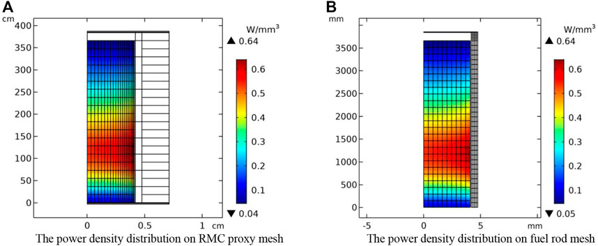
FIGURE 2. Power density distribution on RMC proxy mesh (A) and fuel rod mesh (B).
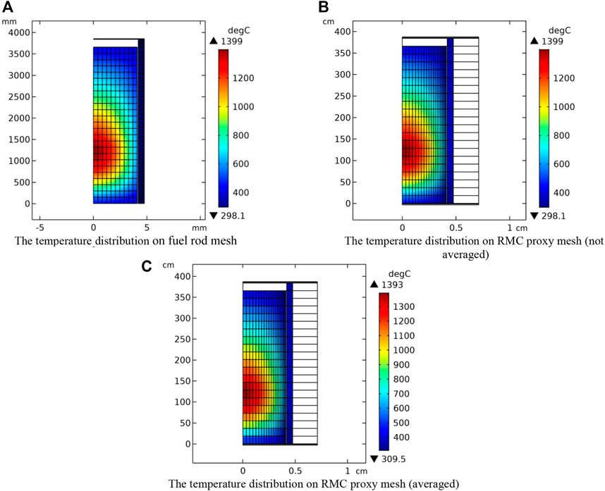
FIGURE 3. Temperature distribution on fuel rod mesh (A), RMC proxy mesh (not averaged) (B) and RMC proxy mesh (averaged) (C).
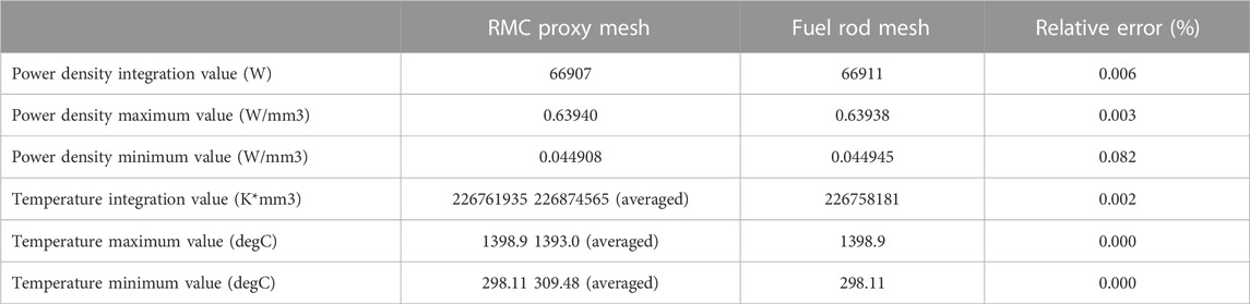
TABLE 1. Statistical values of variables on different meshes.
2.3.3 Coupling control flow
Three different study steps of COMSOL are created to control the running sequences. All three study steps are under the control of the “For” node and “End For” node which are solution utility nodes of COMSOL. The study steps are executed circularly to realize the neutronics and fuel performance calculations iteration. The coupling control flow chart and the specific computation tasks of each step are listed in Figure 4. There are different termination methods for the “For” node, such as fixed number of iterations or convergence of global variable or minimization of global variable. The convergence of effective multiplication factor of RMC is used to determine the termination of iterations for simplification, the convergence formulation is given as:
where
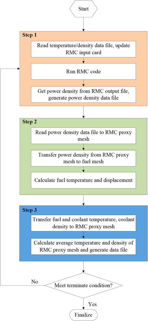
FIGURE 4. Control flow chart of coupling.
3 Demonstration calculations
A typical PWR coupled calculation is used to demonstrate the coupled system. The fuel rod lattice includes UO2 pellet, zircaloy cladding and outside coolant. The steady state coupled problem at the BOL is calculated. Subsequently, with the improvement of the coupled system, it will be further extended to burnup depletion in the whole life cycle. The main modeling parameters are listed in Table 2.
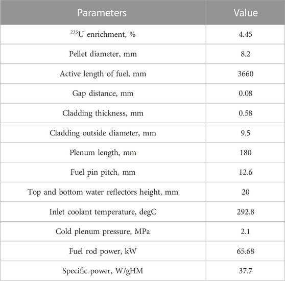
TABLE 2. Main modeling parameters.
3.1 Fuel performance calculation model
The 2D RZ axisymmetric analysis mode is used for the fuel performance calculation, and pellet, cladding and upper end plug are modeled. The detailed pellet geometry is not considered in the modeling to reducing the amount of mesh elements. The flow heat transfer of the coolant is solved axially on the outer surface of the cladding. The pressure boundary conditions are set on the outer surface of the pellet and the inner surface of the cladding, and the load is the internal pressure, which will be update based on the deformed geometry. The constant system pressure is loaded on the outer surface of the cladding. The axial displacement of pellet bottom surface is fixed, and the same for cladding bottom surface.
The outer surface of the pellet and the inner surface of the cladding are set as a contact pair to support the heat transfer and possible mechanical interaction between the pellet and cladding. The inner surface of the cladding is set as destination surface, so the mesh is refined to obtain stable calculation results. The mesh element type for thermal analysis is Lagrange linear, and the mesh element type for mechanical analysis is Lagrange quadratic. This will ensure that the thermal strain is of the same order as the total strain, both first orders. Considering the steep radial power distribution at the edge of the pellet, a non-uniform mesh is used, and the mesh density near the edge is higher. Three different pellet and cladding radial mesh divisions (case 1 (10, 3), case 2 (20, 5), case 3 (30, 7)) were established to study the influence of mesh division on temperature and stress calculation. The results are shown in Figure 5. The temperature and stress vary little from case to case. Considering the balance between efficiency and accuracy, case 2 was selected. The fuel rod mesh parameters are listed in Table 3, and the mesh is shown in Figure 6.

FIGURE 5. Effects of different mesh divisions on fuel rod temperature (A) and von Mises stress (B).
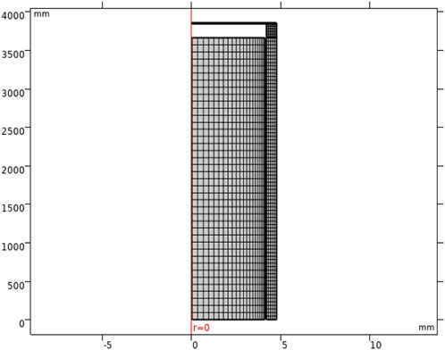
FIGURE 6. Fuel rod mesh used by fuel performance analysis module.
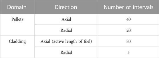
TABLE 3. Fuel rod mesh parameters used by fuel performance analysis module.
3.2 RMC calculation model
Firstly, the proxy mesh of RMC was established in COMSOL, and then the corresponding input card was generated using the RMC input card generation code. The fuel rod lattice mesh parameters are listed in Table 4. A non-uniform division is used to catch the steep radial power distribution at the edge of the pellet. The proxy mesh of RMC in 2D RZ axisymmetric configuration is shown in Figure 7. It is worth noting that the geometry described by RMC is 3D. The pellets, the pellet-cladding gap, the cladding, the upper and lower end plugs, the coolant outside the cladding, and the upper and lower water layers are considered in the RMC modeling. The coolant cylindrical outer surface adopts the total reflection boundary condition, and the boundaries of the bottom and top water reflectors adopt the vacuum boundary condition. This setting approximates a repeating cell arrangement in an infinite space. The representative power distribution will be obtained. If a more accurate distribution is desired, the model needs to scale up to one fuel assembly, or even multiple fuel assemblies, to consider more realistic structural material distributions.
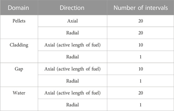
TABLE 4. Fuel rod lattice mesh parameters used by RMC.
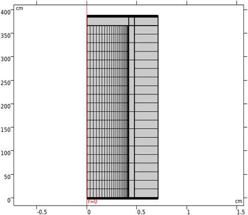
FIGURE 7. Proxy mesh of RMC in COMSOL.
The generations of particles and the number of particles used in the RMC calculation have a significant impact on the calculation results. In this work, the calculation accuracy and efficiency are comprehensively considered, and 1000 are used. The first 200 generations are inactive generations, and the number of particles in each generation is 100000. More initial fission sources in the axial direction can improve the convergence of local power, so 30 initial fission sources are evenly arranged along the axial direction.
4 Results and discussion
4.1 Verification
A simplified case of fuel performance analysis coupled with an external program was constructed to verify the correctness of the coupling methodology proposed in this study. A simple python program was written to represent the calculation of RMC. The program can read the temperature of the mesh element and write the corresponding power density to the hard disk. Assuming that the power density is a function of temperature, the following equation is used to calculate the power density:
Following the coupling methodology described in Section 2.3: 1) the average temperature values on the RMC proxy mesh were exported to data file, 2) the python program read the temperature and written the corresponding power density to date file, 3) the power density values were imported into RMC proxy mesh and transferred to the mesh of fuel performance module, 4) after fuel performance analysis was completed, the temperature values were transferred to the RMC proxy mesh and volume averaged. Then repeat the above steps until the calculation is completed. The external coupling was carried out in this way of Picard iteration. The convergence of fuel rod maximum temperature is used to determine the termination of iterations, relative tolerance 1e-3 is used. After 10 iterations, the convergence requirement was met.
The same case was also solved using COMSOL built-in coupling functionality as reference. Figure 8 shows the comparison of temperature and radial displacement distribution of two coupling methods. The maximum relative deviations for temperature and radial displacement are about 0.15% and 0.79%, indicating that the coupling method proposed in this study is feasible.
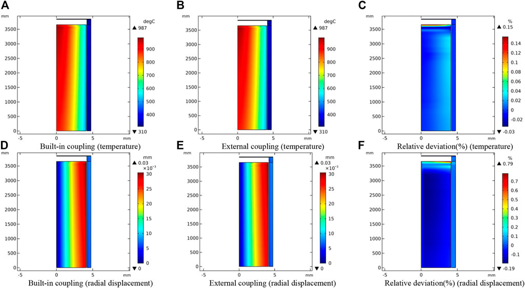
FIGURE 8. Comparison of the temperature (A–C) and radial displacement (D–F) by the two coupling methods.
4.2 Demonstration case
The fuel rod performance analysis and neutronics demonstration case was solved. Figure 9 shows the variation of effective multiplication factor keff with the number of coupling iterations. It is clear that keff reached steady after 3 iterations in the calculation, and the last two results (the 3rd and 4th iteration) are basically identical according to Figure 9, which means the multiphysics coupling problem is converged after only few iterations.
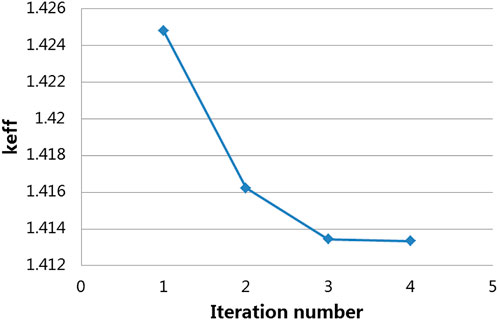
FIGURE 9. Variation of effective multiplication factor with Iteration number.
Power density along the center axis of the fuel rod during iterations was plotted in Figure 10. The power density obtained from RMC under the initial constant temperature filled of 20°C is distributed symmetrically along the axial direction, as illustrated by the blue curve of the first iteration in Figure 10, and the maximum power occurs near the half height of the fuel rod. After that, the peak of power density shifts toward the lower side of the fuel rod in subsequent iterations during calculation. Power density curves other than the initial iteration match well with each other according to Figure 10, especially for results from the last two iterations. Figure 11 shows the coolant temperature and density distribution after convergence, due to the low temperature and high density of the coolant at the lower end, its moderating ability is greater than that of the coolant at the outlet side, so the proportion of thermal neutrons is large, and the fission reaction rate is large. So, the peak of power density is at the lower side of the fuel rod. The coupled Serpent/RELAP5 and DeCart/RELAP5 results for UO2 single assembly BOL were provided in the literature (Wu and Kozlowski, 2015), the results are comparable with this work. The comparison of normalized axial power density distributions is shown in Figure 12. The locations of power peak are almost consistent. There are some differences in the upper part. The discrepancy could be due to several factors, such as differences in models, input parameters or analysis scale (fuel rod lattice vs. single assembly).
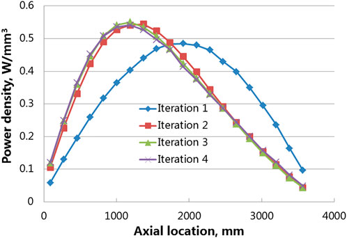
FIGURE 10. Power density along the center axis of the fuel rod during iterations.
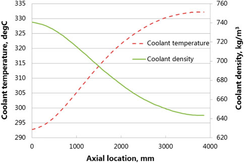
FIGURE 11. Coolant temperature and density distribution after convergence.
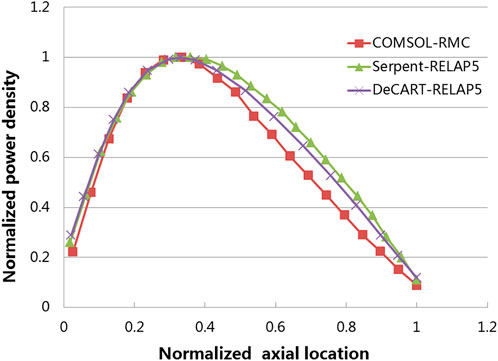
FIGURE 12. Normalized axial power density distributions comparison.
Figure 13 shows distributions of power density (Figure 13A), burnup (Figure 13B), fast neutron flux (Figure 13C), temperature (Figure 13D), cladding hoop stress (Figure 13E) and radial displacement (Figure 13F) in the fuel rod after convergence. The peak of these parameters is located at almost a same height in lower middle area of the fuel rod. The power density and burnup have a similar distribution as expected. The values are higher at the edge of the pellet due to the neutronic rim effect. In contrast, the fast neutron flux is higher in the center of the pellet. The maximum temperature is about 1370°C and occurs in the pellet center of the same height as the peak of power density shown in Figure 13A. Since the external pressure on the cladding is greater than the internal pressure, the cladding is in compressed state, and the hoop compressive stress on the inner side is greater than that on the outer side. Apparently, thermal expansion of the fuel pellets under high temperature is the main driving force for radial displacement during this start-up phase of the reactor. Consequently, the maximum radial displacement or the minimum gap width locates at the height corresponding to the hottest region of the fuel rod, i.e., near 1100 mm in axial direction.
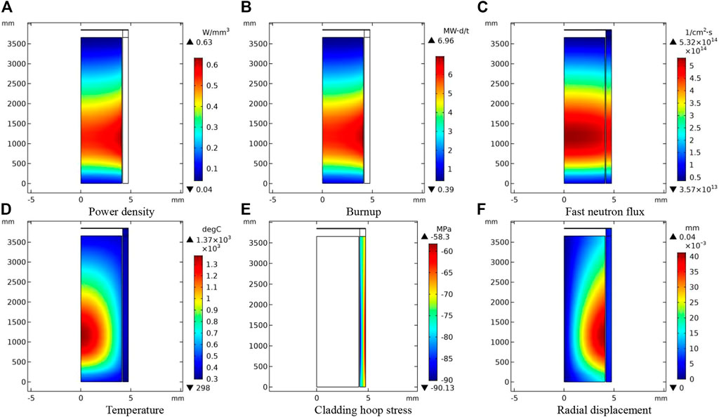
FIGURE 13. Fuel rod performance results: power density (A), burnup (B), fast neutron flux (C), temperature (D), cladding hoop stress (E) and radial displacement (F) after convergence.
The comparison between the radial power distribution obtained by the coupled system and the APOLLO2 data table from COPERNIC fuel performance code (Jacoud and Vesco, 2000) is shown in Figure 14. The APOLLO2 data table values are linearly interpolated between 0MWd/tU and 2000MWd/tU. The power density at the outer edge of the pellet is higher than the inner region as expected. Since the 239Pu is not enriched significantly at the BOL, such radial distribution is mainly caused by self-shielding. The power distribution obtained by the coupled system and the APOLLO2 data table are similar. The value of the coupling result near the edge of the pellet is a bit higher, and the value at the center of the pellet is a bit lower. APOLLO2 data table is related to burnup and radial position. It reflects the average radial power profile of different radial temperature distribution under the same burnup. The radial power profile from coupling system presented in Figure 14 is corresponding to a specific radial temperature distribution. This may be the reason for the discrepancy.
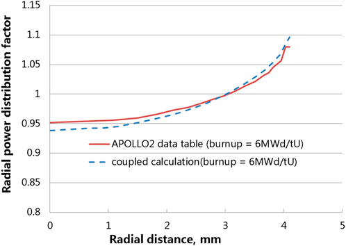
FIGURE 14. Distributions of radial power after convergence.
5 Conclusion
To establish a fuel multiphysics coupling system, a fuel performance analysis module based on the COMSOL Multiphysics software is developed and coupled to Monte Carlo reactor physics code RMC using a novel and robust method. RMC was wrapped as a component of COMSOL to communicate with the fuel performance analysis module. The data transferring and the coupling process was maintained using COMSOL’s functionality. The feasibility of the coupling method is verified using typical case. A fuel rod lattice steady state coupling at the BOL is used to demonstrate the coupled system. Through the coupling of neutronics and fuel performance, axial and radial results are obtained considering temperature feedback, coolant density feedback and self-shielding. Although this is a relatively simple case, the calculation results show the potential of the coupled system. Due to the flexible architecture of the coupled system, it is not limited to a specific fuel type. The performance of new designed fuel rod can be analyzed with reasonable setting using the coupled system. Alternatively, the coupled system could be used to derive the fitting parameters for calibrating the neutronics model for a specific and unusual fuel type to speed up the analysis. As for further improvement of the coupled system, burnup depletion will be included to the coupling and fuel assembly scale coupling will be carried out to test the ability of the system.
Data availability statement
The original contributions presented in the study are included in the article/Supplementary Material, further inquiries can be directed to the corresponding authors.
Author contributions
ZL: methodology, fuel performance module development and data analysis. WiZ: conceptualization and supervision. FQ: coupling interface development. YZ: methodology. QL: validation. PC: supervision. CY: project administration. YL: neutronics modelling. WbZ: neutronics modelling. HW: data analysis and check. YH: data analysis and check.
Funding
This study was supported by the National Key Research and Development Program of China (No. 2022YFB1902300).
Conflict of interest
The authors declare that the research was conducted in the absence of any commercial or financial relationships that could be construed as a potential conflict of interest.
Publisher’s note
All claims expressed in this article are solely those of the authors and do not necessarily represent those of their affiliated organizations, or those of the publisher, the editors and the reviewers. Any product that may be evaluated in this article, or claim that may be made by its manufacturer, is not guaranteed or endorsed by the publisher.
References
CASL (2020). Consortium for advanced simulation of light water reactors (CASL). Available http://www.casl.gov/ (Accessed February 10, 2023).
Clarno, K. T., Hamilton, S. P., Philip, B., Berrill, M. A., Sampath, R. S., Allu, S., et al. (2012). “Integrated radiation transport and nuclear fuel performance for assembly-level simulations,”. ORNL/TM-2012/33.
Gaston, D., Newman, C., Hansen, G., and Lebrun-Grandié, D. (2009). Moose: A parallel computational framework for coupled systems of nonlinear equations. Nucl. Eng. Des. 239, 1768–1778. doi:10.1016/j.nucengdes.2009.05.021
Geelhood, K. J., Lusher, W. G., Raynaud, P. A., and Porter, I. E. (2015). “FRAPCON-4.0: A computer code for the calculation of steady-state, thermal-mechanical behavior of oxide fuel rods for high burnup,”. PNNL-19418, Vol. 1 Rev. 2.
Gleicher, F. N., Spencer, B., Novascone, S., Williamson, R., Martineau, R. C., Rose, M., et al. (2013). Coupling the core analysis program DeCART to the fuel performance application BISON, international conference on mathematics and computational methods applied to nuclear science and engineering. Austria: IAEA.
Gleicher, F., Ortensi, J., DeHart, M., Wang, Y., Schunert, S., Novascone, S., et al. (2016). The application of MAMMOTH for a detailed strongly coupled fuel pin simulation with a station blackout, top fuel 2016, september 2016. USA: Idaho National Laboratory.
Jacoud, J. L., and Vesco, P. (2000). “Description and qualification of the COPERNIC/TRANSURANUS (update of may 2000) fuel rod design code, framatome nuclear fuel,”. TFJCDC1556.
Kramman, E. M., and Freeburn, H. R. (1987). “Escore–the epri steady-state core reload evaluator code: General description,”. Technical Report EPRI NP-5100.
Lassmann, K., O’Carroll, C., van de Laar, J., and Walker, C. T. (1994). The radial distribution of plutonium in high burnup UO2 fuels. J. Nucl. Mater. 208, 223–231. doi:10.1016/0022-3115(94)90331-x
Lee, C. B., Kim, D. H., Song, J. S., Bang, J. G., and Jung, Y. H. (2000). RAPID model to predict radial burnup distribution in LWR UO2 fuel. J. Nucl. Mater. 282, 196–204. doi:10.1016/s0022-3115(00)00408-6
Lusher, W. G., Geelhood, K. J., and Porter, I. E. (2015). “Material property correlations: Comparisons between FRAPCON-4.0, FRAPTRAN-2.0, and MATPRO,”. PNNL-19417 Rev. 2.
MED (2022). MEDCoupling developer's guide, SALOME-platform. Available https://docs.salome-platform.org/latest/dev/MEDCoupling/developer/reference.html (Accessed February 10, 2023).
Olander, D. R. (1976). Fundamental aspects of nuclear reactor fuel elements. Tech. Inf. Cent. Office Public Aff., 137–138.
Palmer, I. D., Hesketh, K. W., and Jackson, P. A. (1982). A model for predicting the radial power profile in a fuel pin, Specialists' meeting on fuel element performance computer modelling. United Kingdom: British Nuclear Fuels Ltd.
Rintala, V., Suikkanen, H., Schubert, A., and Van Uffelen, P. (2022). Supplementing fuel behaviour analyses via coupled Monte Carlo neutronics and fission product solution. Nucl. Eng. Des. 389 (111668), 111668. doi:10.1016/j.nucengdes.2022.111668
Ross, A. M., and Stoute, R. L. (1962). Heat transfer coeffient between UO2 and Zircaloy-2. Canada: Atomic Energy of Canada Technical Report.
Scolaro, Y., Robert, I., Clifford, C., and Fiorina, A. P. (2019). Coupling methodology for the multidimensional fuel performance code offbeat and the Monte Carlo neutron transport code SERPENT, Top Fuel 2019. Seattle, WA.
Suikkanen, H., Rintala, V., Schubert, A., and Van Uffelen, P. (2020). Development of coupled neutronics and fuel performance analysis capabilities between Serpent and TRANSURANUS. Nucl. Eng. Des. 359 (110450), 110450. doi:10.1016/j.nucengdes.2019.110450
Van Uffelen, P., Hales, J., Li, W., Rossiter, G., and Williamson, R. (2019). A review of fuel performance modelling. J. Nucl. Mater. 516, 373–412. doi:10.1016/j.jnucmat.2018.12.037
Wang, K., Li, Z., She, D., Liang, J., Xu, Q., Qiu, Y., et al. (2015). Rmc – a Monte Carlo code for reactor core analysis. Ann. Nucl. Energy 516, 121–129. doi:10.1016/j.anucene.2014.08.048
Weng, M., Liu, S., Liu, Z., Qi, F., Zhou, Y., and Chen, Y. (2021). Development and application of Monte Carlo and COMSOL coupling code for neutronics/thermohydraulics coupled analysis. Ann. Nucl. Energy 161 (108459), 108459. doi:10.1016/j.anucene.2021.108459
Keywords: multiphysics coupling, fuel performance, fuel rod, COMSOL, RMC
Citation: Liu Z, Zeng W, Qi F, Zhou Y, Li Q, Chen P, Yin C, Liu Y, Zhao W, Wang H and Huang Y (2023) Development of multiphysics coupling system for nuclear fuel rod with COMSOL and RMC. Front. Energy Res. 11:1145046. doi: 10.3389/fenrg.2023.1145046
Received: 15 January 2023; Accepted: 15 February 2023;
Published: 27 February 2023.
Edited by:
Shichang Liu, North China Electric Power University, ChinaReviewed by:
Di Yun, Xi’an Jiaotong University, ChinaRong Liu, South China University of Technology, China
Liuxuan Cao, Xiamen University, China
Yanan He, Xi’an Jiaotong University, China
Copyright © 2023 Liu, Zeng, Qi, Zhou, Li, Chen, Yin, Liu, Zhao, Wang and Huang. This is an open-access article distributed under the terms of the Creative Commons Attribution License (CC BY). The use, distribution or reproduction in other forums is permitted, provided the original author(s) and the copyright owner(s) are credited and that the original publication in this journal is cited, in accordance with accepted academic practice. No use, distribution or reproduction is permitted which does not comply with these terms.
*Correspondence: Zhenhai Liu, MTk4OWx6aGhAc2luYS5jb20=; Wei Zeng, emVuZ3dlaTAyQHNpbmEuY29t