 Dingwen Lu
 Zhihong Ren
 Jianwei Yang*
- School of Electrical Engineering, Southwest Jiaotong University, Chengdu, China
With high penetration of wind power, the apparent inertia of power systems is decreased, which seriously affects the safety and stability of the system frequency. Therefore, a novel sliding mode frequency control (SMFC) scheme is proposed for the wind turbines participating in frequency regulation support (FRS) in power systems, which can significantly improve the dynamic characteristics of the system frequency. At first, a power system frequency response model considering wind turbines participation in FRS is derived. In this model, the load disturbance, wind power disturbance and synchronous generator frequency regulation dynamics are combined as a lumped disturbance. Then, the design of the proposed SMFC scheme, which combines the super-twisting sliding-mode disturbance observer (STSMDO) with the super-twisting sliding-mode frequency controller (STSMFC), is introduced. The proposed STSMFC has ability to tune the system dynamics easily by choosing suitable sliding surface matrix via eigenvalue assignment method or optimal sliding manifold design. In such a frequency control scheme, the stability of the system frequency is guaranteed by the STSMFC, whereas the STSMDO is employed to estimate the lumped disturbance. Finally, numerical simulations verify the effectiveness and superiority of the proposed SMFC scheme.
1 Introduction
As a clean and pollution-free renewable energy, wind power has been rapidly utilized to cope with growing energy demand and environmental problems. At the end of 2020, the global installed capacity of it has exceeded 700 GW (Global Wind Energy Council, 2021). But the wind power is connected to the grid through a back-to-back full-power pulse width modulation (PWM) converter and generally works in the maximum power point tracking (MPPT) mode (Gaied et al., 2022). The rotor speed of wind power generator is decoupled from the grid frequency unlike traditional synchronous generators (SGs) (Fan et al., 2021). And wind power cannot provide frequency regulation support (FRS) for the power system. Thus, under a high wind power penetration level (WPPL), the apparent inertia of the power system is reduced and may lead to power system oscillations (Wang, Silva, & Lopez-Botet-Zulueta, 2016). In addition, due to the influence of wind speed, the output of wind power has strong uncertainty, which further strengthens the difficulty of frequency control. As a result, the power system with high WPPL is faced with the severe problem of insufficient FRS capacity.
In order to improve the FRS capacity of power system with high WPPL, using wind turbines (WTs) to participate in FRS has been vigorously developed in many countries (Wang & Tomsovic, 2018), since WTs have a faster response speed than traditional SGs in terms of power regulation (Morren, de Haan, Kling, & Ferreira, 2006; Wu, Yang, Hu, & Dzung, 2019). Therefore, some researchers propose virtual inertial control which mimics the inertial response of SGs by quickly releasing kinetic energy on the WT (Ochoa & Martinez, 2017; Zeng, Liu, Wang, Dong, & Chen, 2019; Xi, Geng, & Zou, 2021) and de-loading control which obtains the power reserve by making WTs de-loading operation for FRS (Arani & Mohamed, 2018; Gholamrezaie, Dozein, Monsef, & Wu, 2018; Abazari, Monsef, & Wu, 2019). In (Ochoa & Martinez, 2017; Zeng et al., 2019; Xi et al., 2021), the proportional-derivative (PD) controller is applied to provide inertial support for reducing the rate of change of frequency (RoCoF). Combining droop control and de-loading control, dynamic droop control is proposed in (Arani & Mohamed, 2018) to provide short-term (primary) frequency regulation and improve frequency nadir (FN). To further achieve long-term (secondary) frequency regulation, a frequency controller is designed for WTs to improve the system frequency performance, which is essentially a proportional-integral-derivative (PID) controller with optimization algorithm (Gholamrezaie et al., 2018; Abazari et al., 2019). However, in the above method, the frequency control adopts a PD or PID controller, which is a linear controller. From a practical point of view, the frequency dynamics of the power system with high WPPL is a time-varying non-linear system subject to various disturbances, including external disturbances, parameter uncertainties, and unmodeled dynamics. Since classical PD or PID controller is sensitive to time-varying disturbances, the use of such controllers for frequency control leads to unsatisfactory dynamic performance. Hence, there is a need to employ non-linear control methods for frequency controller in the power system with high WPPL, such as predictive control (Kou, Liang, Yu, & Gao, 2019; Kayedpour, Samani, De Kooning, Vandevelde, & Crevecoeur, 2022), robust control (Liu & Ma, 2018; Roozbehani, Hagh, & Zadeh, 2019), sliding mode control (SMC) (Mi et al., 2017; Prasad, Purwar, & Kishor, 2019; Deng & Xu, 2022), etc.
Among the above non-linear control methods, SMC is widely concerned in power engineering and is considered as an effective method to deal with the uncertainty of non-linear system, as it has advantages of fast response speed and high robust performance against uncertain systems (Evangelista, Valenciaga, & Puleston, 2013; Liao et al., 2017; Ding, Chen, Mei, & Murray-Smith, 2020). And compared with traditional PID controller, the dynamics of SMC can be designed regardless of the uncertainties of system parameters and disturbances, which enhances the robustness of SMC (Liao & Xu, 2018). This is also the reason why this method is selected. To improve the robustness and stability of the power system with high WPPL, a decentralized sliding mode load frequency control (LFC) strategy is proposed in (Mi et al., 2016) to mitigate large disturbances. But it only considers the traditional SGs to provide FRS, which is difficult to respond to power system with high WPPL effectively today. Besides, the decentralized sliding mode LFC strategy is based on a first-order sliding mode algorithm, which may suffer from chattering phenomenon. In (Prasad et al., 2019; Deng & Xu, 2022), the sliding mode controller is designed for traditional SGs and WTs, respectively, to jointly participate in the FRS. But the lumped disturbance is assumed to be known in the controller design. Since the lumped disturbance is unmeasured in the practical power system with high WPPL, it is necessary to estimate the lumped disturbance for the sliding mode controller design. The traditional disturbance estimation method is to design a disturbance observer (DOB) (Mi, Song, Fu, & Wang, 2020; Wang, Mi, Fu, & Wang, 2018; Yang et al., 2021). By taking advantage of the DOB and sliding mode law, the sliding mode controller is designed to improve dynamic performance of the power system with wind power (Mi et al., 2020; Wang et al., 2018). Based on the lumped disturbance estimated by DOB, the fractional-order integral sliding mode controller is constructed to relieve the chattering of frequency deviation and tie-line power deviation in the interconnected power system with wind power (Yang et al., 2021). However, the DOB is difficult to deal with the system uncertain. Therefore, it is necessary to design a disturbance observer with sliding mode algorithm for power system with high WPPL. Furthermore, the estimated disturbance can be used to design sliding mode surfaces.
In this paper, to improve the dynamic characteristics of the system frequency, a novel sliding mode frequency control (SMFC) scheme is proposed for the WTs participating in FRS in power systems. At first, a power system frequency response model with WTs participating in FRS is derived. In this model, the load disturbance, wind power disturbance and frequency regulation dynamics of SGs are combined as a lumped disturbance, and the WT is in de-loading operation for obtaining power reserve through over-speed de-loading control. Then, the disturbance observer and frequency controller are designed as STSMDO and STSMFC based on the super-twisting sliding mode (STSM) algorithm, which can effectively avoid the chattering problem. In such a frequency control scheme consisting of STSMDO and STSMFC, the desired dynamic performance of the system frequency is guaranteed by the STSMFC, whereas the STSMDO is employed to estimate the lumped disturbance, which is used to design the sliding mode surface of STSMFC. Finally, numerical simulation is carried out to test the proposed SMFC scheme.
The main contributions of this work can be summarized in two aspects. On the one hand, a STSMDO is designed to estimate lumped disturbances in power systems with high WPPL, which can achieve better observational performance than traditional DOB. On the other hand, by designing a new sliding mode surface, a STSMFC is developed for WTs, which has ability to tune the system frequency dynamics easily by choosing suitable sliding surface matrix via eigenvalue assignment (EA) method or optimal sliding manifold (OSM) design.
The remainder of the paper is organized as follows. Section 2 introduces the power system frequency response model with WTs participating in FRS and problem formulation. In Section 3, the proposed SMFC scheme is given, which consists of STSMDO and STSMFC. The stability of the system is analyzed in Section 4. Section 5 shows the simulation results. Finally, conclusion are given in Section 6.
2 System modeling and problem formulation
As large-scale wind power is connected to the power system, SGs are no longer dominant in the FRS. Therefore, it is necessary to incorporate the WTs participating in FRS into the system frequency response model. This model is depicted in Figure 1, which consists of a power system frequency response model, a wind turbine linearization model and the proposed SMFC scheme. It is worth noting that the turbine can be selected as reheat turbine or steam turbine, neither of which will affect the proposed SMFC scheme. Here, take the steam turbine as an example. The parameters dw and ds (1-dw) are the WPPL and penetration level of SGs respectively. They can be simply modified to simulate different WPPLs. The input of the model is the system uncertainty disturbance composed of load disturbance and wind speed disturbance, and the output is the system frequency deviation. It can simply and accurately reflect the system frequency dynamics with WTs participating in FRS.
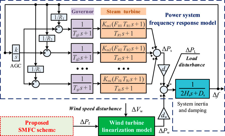
FIGURE 1. Power system frequency response model with WTs participating in FRS.
2.1 Power system frequency response model
The power system frequency response model can describe the system frequency deviation, which is made up of governor, steam turbine, automatic generation control (AGC) unit, system inertia and damping. Under the large-scale access of wind power, the system inertia can be expressed as (Kayedpour et al., 2022)
where i is the number of SG, N is the total number of SG before the wind power is connected, Si and Hi are the rated power and inertia time constant of the i-th SG, dw is the WPPL, Ssys is the system installed capacity. It can be seen from Eq. 1 that when dw is larger, the system inertia is smaller, which will threaten the security and stability of the system frequency.
The frequency regulation dynamics of SGs can be described as
where k is the AGC parameter, R is the speed drop, FH is fraction of total power generated by the HP turbine, Km is mechanical power gain factor, Tg and TR are the time constant of the governor and steam turbine, respectively.
Therefore, the system frequency deviation of the power system can be deduced as
where ΔPw is wind power deviation, ΔPL is load disturbance, Ds is damping.
2.2 Wind turbine linearization model
As shown in Figure 2, the proposed wind turbine linearization model can reflect the dynamic behavior
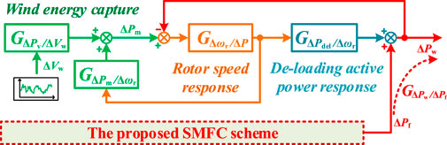
FIGURE 2. Wind turbine linearization model.
2.2.1 De-loading operation of the WT
Under MPPT control, the mechanical power Pm and tip speed ratio λ can be expressed as
where R is the blade length, ρ is the air density and Vw is the wind speed. And p, kg, ωr are the number of pole pairs, the gearbox ratio and the rotor speed respectively. When the tip speed ratio λ maintains the optimal tip speed ratio, the wind power conversion coefficient CP is the maximum and WTs can obtain maximum wind power, which can be described as
where k0, k1, and k2 are constant coefficients.
According to Eqs 4, 5, the maximum power captured by WTs can be calculated as
where ωropt is the optimal rotor speed, kopt is the optimal coefficient.
For obtaining reserved mechanical power for FRS, the over-speed de-loading control is used to make the WT in de-loading operation in this paper, which can adjust the power output faster than the pitch angle control. The de-loading active power is obtained as (Liao, Xu, Wang, & Lin, 2019)
where kdel,
2.2.2 Linearization of the WT
The wind turbine linearization model is the basis for designing the proposed SMFC scheme. The small signal analysis method is used to linearize the WT. For wind energy capture part, it is affected by the variation of wind speed ΔVw and rotor speed Δωr. Thus, select Vw0 and ωrdel0 at the stable working point of the WT, and linearize the wind energy capture dynamics caused by wind speed variation ΔVw and rotor speed variation Δωr respectively, which can be expressed as
where
Considering that the de-loading active response part is only related to the rotor speed Δωr. Therefore, ωrdel0 is also selected as the stable point, and the linearized de-loading active response dynamics can be obtained as
where
For representing the rotor dynamics, the single-mass rotor model is selected here, and the linearized rotor speed response part concerning the unbalanced power ∆P between electromagnetic active power ∆Pdel and mechanical power ∆Pm can be expressed as
where Hw is the inertial constant, and Dw is the damping.
Eventually, based on Figure 2 and Eqs 8–11, the dynamic behavior of the WT to the ΔPf and the ΔVw are as follows
where Aw = (ωrdel0Dw—
2.2.3 System frequency dynamics of the power system with WTs participating in FRS
Based on Eqs 2, 3, 12, 13, through the deformation of WTs frequency response transfer function
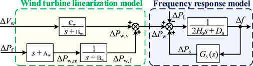
FIGURE 3. Structure of the simplified frequency response model of the power system.
Thus, the system frequency dynamics of the power system with WTs participating in FRS can be expressed as
where ∆Pw,f is the power provided by the WT for FRS, ∆Pw,m is the intermediate variable of the ∆Pw,f, ∆Pd = ∆PL-∆Ps-∆Pw,v is the lumped disturbance, ∆Pw,v is the wind power disturbance caused by wind speed disturbance.
The system frequency dynamics can also be rewritten as the matrix form:
where the state variable matrix ∆x = [∆f ∆Pw,f ∆Pw,m]T, the control term u = ∆Pf,
The goal of this paper is to keep the system frequency deviation, ∆f, to zero by WTs providing the FRS. As illustrated in Eq. 17, Maintaining ∆f to zero in the presence of load disturbance and wind speed disturbance means regulating the power provided by the WT for FRS, ∆Pw,f, to track the lumped disturbance which is estimated from the STSMDO, ∆Pd, by regulating the control input ∆Pf. Therefore, the frequency control against load disturbance and wind speed disturbance can both be treated as a tracking control problem in the presence of SG.
Remark 1: Integrating ∆Ps into the lumped disturbance ∆Pd has two benefits. One benefit is that there is no need to collect decentralized SGs power information. The other is that the cooperative work between WTs and SGs can be linked by the lumped disturbance. When the disturbance (load disturbance or wind power disturbance) occurs, the SGs participate in the FRS, and the lumped disturbance is correspondingly reduced. It is the reduced lumped disturbance that is the tracking target of WTs. Therefore, WTs can cooperate with SGs to provide the FRS for power systems with high WPPL.
3 Proposed SMFC scheme
The system frequency is unavoidably affected by various uncertainty disturbances. As mentioned before, the traditional PID control is not easy to achieve a satisfactory performance under various uncertainty disturbances. It is known that SMC has been proven to be an effective non-linear control method for uncertainty systems and incompletely modeled systems, though there is a chattering problem. To fix this problem, the second-order sliding mode algorithm is selected, namely the STSM algorithm, which can effectively deal with the chattering problem and eliminates the need to measure the derivative of the sliding variable (Evangelista et al., 2013; Liao & Xu, 2018). Meanwhile, the sign function is smoothed in the STSM algorithm, which is devoted to reducing chattering effects. Here, the diagram of the proposed SMFC scheme is depicted in Figure 4. It includes the STSMDO design and STSMFC design. The STSMDO is used to estimate the lumped disturbance required for the design of the sliding surface matrix K of the STSMFC. The accurate estimation of lumped disturbance can be realized only by external system frequency information and internal STSMFC control information. Based on the lumped disturbance estimated by STSMDO, system parameter matrix and state variable matrix, the STSMFC uses the sliding surface matrix K and the super-twisting sliding mode algorithm to adjust the FRS power ∆Pw,f of WT.
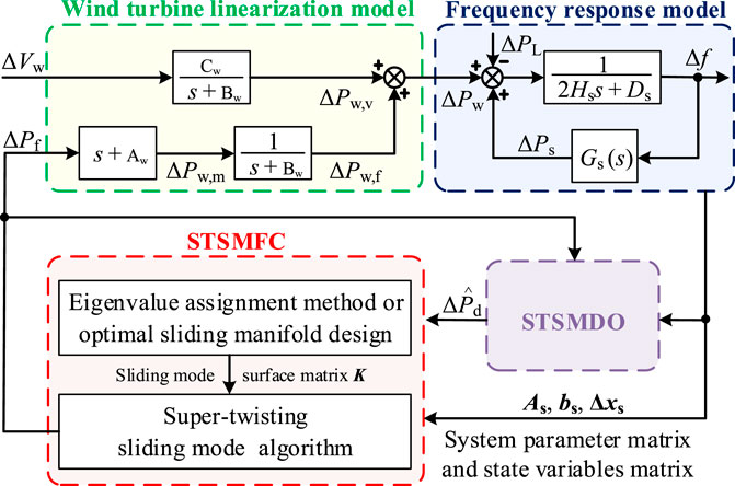
FIGURE 4. Diagram of the proposed SMFC scheme.
In the proposed SMFC scheme shown in Figure 4, its advantage is that the desired system frequency response performance can be achieved only by adjusting the sliding surface matrix K of STSMFC through EA method or OSM design. Under the designed sliding surface matrix K, the STSMFC utilizes the STSM algorithm to force the system to trajectory the predefined sliding surface. When the sliding surface arrives, as mentioned before, the control objective that FRS power ∆Pw,f of WT fast tracks the lumped disturbance ∆Pd can be achieved. In addition, the proposed SMFC scheme has the characteristic of using STSMDO for lumped disturbance estimation. Thus, external information of the proposed SMFC scheme only needs system frequency information for the actual system without other complicated information. For the actual system, this reduces the difficulty of implementation.
3.1 STSMDO design
In the practical power system, the lumped disturbance ∆Pd is usually difficult to measure and it can be replaced by approximate values, which may lead to lower control accuracy. Therefore, the STSMDO is constructed to estimate the unmeasured lumped disturbance. With the estimated results, the proposed sliding variable and sliding surface can be established.
With the system frequency dynamics, as shown in Eq. 14, the STSMDO used to estimate ∆Pd can be designed as:
where
where ρ1 and ρ2 are the positive constant gains of the STSMDO, ef = ∆f—
where σ is a very small positive constant. When the sliding mode variable is too large away from the sliding mode surface, the positive constant will hardly affect the output of the sign function. When the sliding mode variable is close to the sliding mode surface, the positive constant can reduce the output of the sign function, thus weakening the chattering of the sliding mode variable motion track.
Based on Eqs 14, 18, the estimation error dynamics for the STSMDO can be described as the following standard form of the super-twisting algorithm
where ed = ∆Pd—
Assumption 1. The differentiation of lumped disturbance
where ||·||2 is Euclidean norm, ψ = [−ρ1 2]T, and λmin{Uw} represents minimum eigenvalue of the symmetric and positive definite matrix Uw, which is designed as
The stability of the STSMDO is proved in Section 4 based on Lyapunov method.
3.2 Sliding mode surface design
In order to ensure the stability of the system frequency, the various powers in the power system should be kept in balance. When the load disturbance ∆PL or wind power disturbance ∆Pw,v occurs, the frequency controller forces the system state variable track ∆f = 0 and ∆Pw,f =
Substituting Eq. 24 into Eq. 17, the system frequency dynamics can be transformed to the following regular form:
where
Based on the sliding mode variable, when the system dynamic motion is constrained to the sliding mode surface sw = 0 by adjusting the control term u to make Δζ = KΔxs, the system frequency dynamics shown in Eq. 25 can be transformed as
Obviously, for the linear system shown in Eq. 27, the desired performance can be obtained by designing the matrix K to configure the eigenvalues of the matrix Acl. In general, some linear system control design methods can be used, such as the EA method or OSM design (Utkin, 2013). In this paper, the linear quadratic regulator (LQR) method is chosen to design the matrix K for obtaining the OSM. Moreover, to achieve the optimal control effect, the cost function is selected as
where QL ∈ ℝ2×2, NL ∈ ℝ2×1, and RL ∈ ℝ1 are weight matrices, which together determine the importance of the state vector Δxs and the input vector Δζ.
By deforming Eq. 28, the cost function of standard quadratic criterion can be obtained as
where intermediate variable
To minimize the cost function J, the matrix K can be designed based on the Riccati equation as
where P is the unique solution of the associated Riccati equation, which can be obtained by
Remark 3: Driven by the sliding mode control, the system dynamic motion is constrained on the designed sliding mode surface sw = 0, so that the tracking control problem can be solved by the linear system control design method. Here, in order to complete the tracking control objective, the LQR method is selected to force the state vector Δxs = 0 with the desired control cost. In addition, the desired state component tracking error and control cost can be flexibly adjusted by selecting an appropriate weight matrix.
3.3 STSMFC design
The key to achieving the control goal is to ensure that the system is driven to the sliding mode surface, for which the controller of STSMFC u = ue + us is constructed as
where ue is the equivalent control term that transforms the system Eq. 25 into the form of only the state vector Δxs and the sliding mode variable sw, us is the sliding mode control term that forces the system to the sliding mode surface, v represents the sliding mode reaching law based on the super-twisting algorithm, which can be expressed as
where γ1 > 0 and γ2 > 0 are positive constant gains of sliding mode reaching law v.
Furthermore, the system shown in Eq. 25 can be rewritten into the form containing only the state vector Δxs and the sliding mode variable sw, as
where perturbation term
Assumption 2. The differentiation of perturbation term
where φ = [−γ1 2]T, and λmin{Nw} represents minimum eigenvalue of the symmetric and positive definite matrix Nw, which is designed as
Hence, the system can reach the sliding surface within a finite time under any initial condition. Likewise, the stability of the STSMFC is proved in Section 4 based on Lyapunov method.
4 Stability analysis
The premise of achieving the control objective is that the entire system can converge to a steady state. In this section, based on the Lyapunov method, it is verified that STSMDO and STSMFC are converged and stable, and all system trajectories can converge to the origin in finite time.
Theorem 1. Based on Assumption 1, if ρ1 and ρ2 are selected as Eqs 22, 23, ef and ed will converge to the origin in a finite time.
Proof. For the STSMDO of sliding variable dynamics shown in Eq. 21, the candidate Lyapunov function V1 can be selected as follows
where ς = [ς1 ς2]T = [|ef|1/2sign (ef) ed]T, α is a symmetric and positive definite matrix. Thus, the following inequality holds
where λ{α} represents the eigenvalue of matrix α, and the subscripts “max” and “min” represent the maximum and minimum eigenvalues of matrix α, respectively.The time derivative of Lyapunov function V1 along the vector ς can be obtained as
where |ς1| ≤ (ς21 + ς22)1/2 = ||ς||2.Since Uw is also a symmetric positive definite matrix, it can be concluded that λ{Uw} > 0. Therefore, based on Assumption 1; Eqs 39, 40, the following inequality holds
where ε is represented as
Combining Eqs 41, 42, in order to satisfy
Theorem 2. Under the parameter conditions in Eqs 36, 37, for any initial condition, all trajectories of the system Eq. 34 will converge to the sliding surface sw = 0 in finite time.
Proof. For the STSMFC of sliding variable dynamics shown in Eq. 34, the candidate Lyapunov function V2 can be selected as follows
where ξ = [ξ1 ξ2]T = [|sw|1/2sign (sw) z]T, β is a symmetric and positive definite matrix.Obviously, the candidate Lyapunov functions V2 and V1 are similar, so the proof process is also the same, which can be directly obtained as
where δ is represented as
Similarly, when the value ranges of γ1 and γ2 satisfy Eqs 35, 36, it can be concluded that δ < 0,
5 Simulation and results
In this section, the power system model with the novel scheme shown in Figure 1 is simulated in MATLAB/SIMULINK to test the effectiveness of the proposed SMFC scheme under uncertainty disturbances. The test system includes the power system frequency response part and the wind turbine linearization part, which can reflect the frequency dynamics of WTs participating in FRS. The parameters of power system and the WT (Liao, Lu, Wang, & Yang, 2022) used in this test are shown in Tables 1, 2 respectively. In the simulation test, The WPPL dw is equal to 50%. Thus, the test system is a high WPPL system. Under the de-loading ratio of 0.9, the WT has a margin of 0.1 for FRS. For the OSM, the parameters of matrix K can be obtained by LQR method. The damping under various parameters of sliding surface matrix K is shown in Figure 5. For the linear system of Eq. 27, it is expected to have a slow and small change, that is, the frequency deviation Δf and WT tracking error Δη are very small. Therefore, in this test, the damping ratio is selected to be greater than 1, becoming an over-damping system. The parameter design of K is [-60.14–63.55], and the damping ratio is 8.93. Based on the stability constraint range of Eqs 22, 36, and the expected convergence rate, the STSMDO and STSMFC parameters are set as: ρ1 = 1248, ρ2 = 2912, γ1 = 2420, γ2 = 62.89 respectively.

TABLE 1. Parameters of Power system.
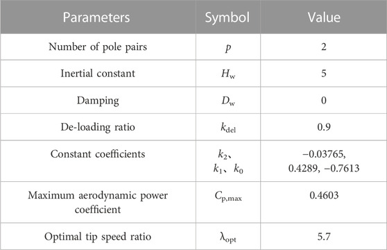
TABLE 2. Parameters of DFIG-based WT.
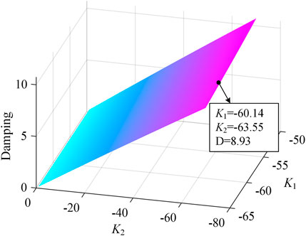
FIGURE 5. Damping under various parameters of sliding surface matrix K.
There are two cases to test the performance of the proposed SMFC scheme. In case one, under the uncertain disturbance of load or wind speed, the proposed SMFC scheme is compared with the optimal frequency control (OFC) in (Gholamrezaie et al., 2018). And the STSMDO is compared with generalized extended state observer (GESO) in (Yang et al., 2021). In case two, under the same uncertain disturbance conditions as in case 1, the proposed SMFC scheme is compared with sliding mode load frequency control (SMLFC) scheme in (Mi et al., 2016).
5.1 Case 1: compared with the OFC
The uncertain disturbance of load or wind speed is the most common uncertain disturbance faced by the power system with high WPPL. In this case, to verify the effectiveness of the proposed SMFC scheme compared with OFC, the simulation system will face the uncertain load and wind speed disturbance shown in Figure 6. The uncertainty load disturbances of 0.0278, −0.01854 and 0.03707 occurred at t = 50, 70, and 100 s respectively. And when t = 125s, the load disturbance is recovered. The uncertainty wind speed disturbance starts at t = 50 s.
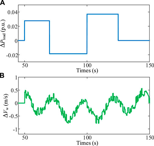
FIGURE 6. Uncertain disturbance. (A) Uncertain load disturbance. (B) Uncertain wind speed disturbance.
The comparison results of disturbance observation and system frequency fluctuation under uncertain load disturbance are shown in Figures 7, 8 respectively. Under uncertain wind speed disturbance, the comparison results are shown in Figures 9, 10 respectively.
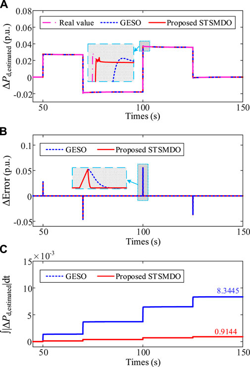
FIGURE 7. Comparison results of the disturbance observation between the STSMDO and the GESO under uncertain load disturbance. (A) Lumped disturbance estimated result. (B) Estimation error. (C) Total estimation error ∫|ΔPd,estimated|dt.
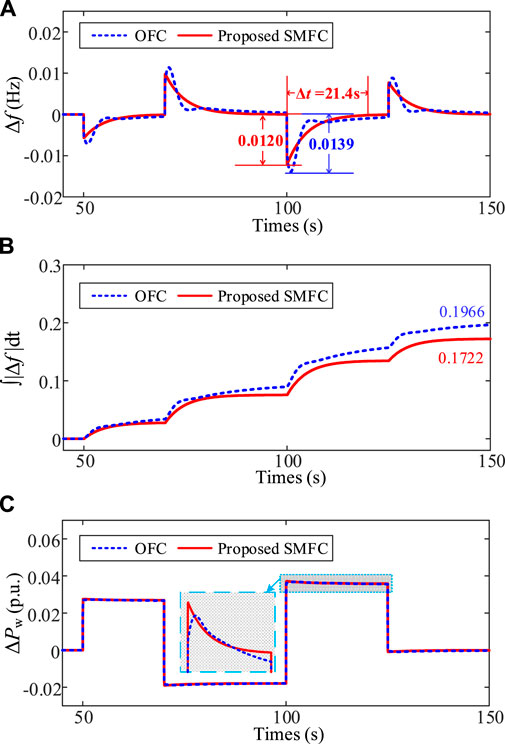
FIGURE 8. Comparison results of the system frequency fluctuation between the STSMFC and the OFC under uncertain load disturbance. (A) System frequency fluctuation. (B) Total frequency fluctuation level ∫|Δf |dt. (C) Wind power deviation.
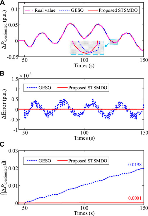
FIGURE 9. Comparison results of the disturbance observation between the STSMDO and the GESO under uncertain wind speed disturbance. (A) Lumped disturbance estimated result. (B) Estimation error. (C) Total estimation error ∫|ΔPd,estimated|dt.
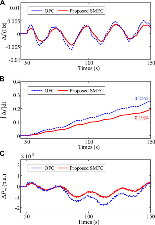
FIGURE 10. Comparison results of the system frequency fluctuation between the SMFC and the OFC under uncertain wind speed disturbance. (A) System frequency fluctuation. (B) Total frequency fluctuation level ∫|Δf |dt. (C) Wind power deviation.
It can be seen from Figure 7A that both the STSMDO and the GESO can estimate the lumped disturbance of the system, and the observation result estimated by proposed STSMDO is more similar to the real lumped disturbance of the system than GESO. Figures 7B, C clearly show that the total estimation error of the proposed STSMDO is smaller and the estimation speed is faster. Thus, the real lumped disturbance can be estimated by the proposed STSMDO approximately, and the lumped disturbance estimated result can be applied in STSMFC.
The effect of the FRS is shown in Figure 8A. Each time load disturbance occurs, the maximum frequency deviation of the proposed SMFC scheme is smaller than that of OFC, and the frequency deviation can be eliminated more quickly and smoothly. Taking the effect of the FRS at 100 s as an example, it can be found that the maximum frequency deviation under the proposed SMFC scheme and OFC is 0.0120Hz and 0.0139 Hz respectively. And the frequency deviation under the proposed SMFC is adjusted to 0 smoothly within 21.4 s, while OFC needs more than 25 s. None is as good as the proposed SMFC scheme. As shown in Figure 8B, the total frequency fluctuation level gradually increases with time. The total frequency fluctuation level under the proposed SMFC scheme is 0.1722. The corresponding value of OFC is 0.1966. It can be seen from Figure 8C that the wind power response under the proposed SMFC scheme is larger than the OFC. This is due to the strong disturbance-rejection ability of the proposed SMFC. These results show that the proposed SMFC scheme significantly improves frequency dynamic performance. In addition, under OFC, the frequency regulation power of wind power will be reduced due to the reduction of frequency deviation, which is difficult to achieve the ideal frequency regulation performance. This is the drawback of PID controller. It is worth noting that the proposed control scheme takes the frequency deviation equal to zero as the target, and the frequency regulation power of wind power is used to quickly track the lumped disturbance. Therefore, the proposed control scheme will not be affected by the reduction of frequency deviation, so as to achieve an ideal frequency regulation effect.
Figures 9A, B show that STSMDO and GESO can also track the lumped disturbance under wind speed disturbance, and STSMDO can also track the actual value more quickly and accurately. It can be seen from Figure 9C that the total error of STSMDO is 0.0001, which is significantly less than the total error of GESO of 0.0198. On the whole, the total error under wind speed disturbance is significantly less than that under load fluctuation. The reason is that the built high-precision wind turbine linearization model is included in the construction of the STSMDO, which can more accurately reflect the output change of the WT.
It can be seen from Figures 10A, B that the frequency fluctuation range under the proposed SMFC scheme is significantly smaller than that under OFC. And the frequency fluctuation is more smooth. The total frequency fluctuation level under OFC is 0.2565. The corresponding value under SMFC is 0.1924, which is reduced by 24.99% compared with OFC. The wind power output is shown in Figure 10C. Under OFC, although the power fluctuation is similar to that under the proposed SMFC scheme in the early stage, there is more obvious power fluctuation in the later stage, which also causes the power balance of the system to be damaged. Thus, the frequency fluctuation is conspicuous. The reason is also due to the drawback of PID controller that will weaken the frequency regulation effect as the frequency deviation decreases. For the proposed SMFC, the wind power output is smoother, so the impact on the system frequency is even smaller. Therefore, it can be seen from the above results that the proposed SMFC can quickly smooth the wind power output according to the frequency deviation and the lumped disturbance power, so as to effectively deal with the impact of uncertain wind speed disturbance on the system frequency.
5.2 Case2: compared with the SMLFC
In this case, the proposed SMFC scheme is compared with SMLFC scheme. To compare the SMLFC schemes applied to non-reheat units, three steam turbines and three governors of test system shown in Figure 1 can be replaced by a non-reheat turbine and a governor. The time constant of the non-reheat turbine and the governor is selected as 0.273, 0.0728 (Mi et al., 2016). Since the observer of the SMLFC scheme is also GESO, the performance of the observer will not be compared here. Similarly, the uncertain load and wind speed disturbance shown in Figure 6 is selected. The comparison results of system frequency fluctuation under uncertain load and wind speed disturbance are shown in Figures 11, 12 respectively.
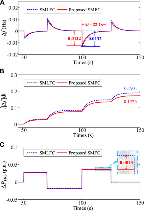
FIGURE 11. Comparison results of the system frequency fluctuation between the SMFC and the SMLFC under uncertain load disturbance. (A) System frequency fluctuation. (B) Total frequency fluctuation level ∫|Δf |dt. (C) Power output deviation of FRS.

FIGURE 12. Comparison results of the system frequency fluctuation between the SMFC and the SMLFC under uncertain wind speed disturbance. (A) System frequency fluctuation. (B) Total frequency fluctuation level ∫|Δf |dt. (C) Power output deviation of FRS.
Figure 11A shows the effect of the FRS between the SMFC and the SMLFC under uncertain load disturbance. In like wise, taking t = 100s as an example, it can be seen that the maximum frequency deviation of the proposed SMFC is 0.0122Hz, and the frequency deviation is adjusted to 0 within 22.1s smoothly. For SMLFC, the correlation values are 0.0132Hz and 22.1s respectively. The total frequency fluctuation level is shown in Figure 11B. The value of the proposed SMFC and SMLFC are 0.1725 and 0.1901 respectively. It can be seen from Figure 11C that the power output deviation of FRS under the proposed SMFC is smaller than the SMLFC. The reason is that SMLFC can only undertake all frequency regulation tasks, and the proposed SMFC scheme can work with the SGs to jointly frequency regulation. This can further utilize the frequency regulation power of the power system. The above results verify that the proposed SMFC scheme has stronger frequency dynamic performance than SMLFC. Compared with OFC in case 1, the maximum frequency deviation and total frequency fluctuation level under the SMLFC are improved by 5.04% and 3.31% respectively. And as with the proposed SMFC scheme, it is not limited by PID controller, and the frequency deviation under SMLFC can reach 0 within 22.1s. Under the proposed SMFC scheme, the maximum frequency deviation, adjustment time and total frequency fluctuation level compared with case 1 have deteriorated, increasing by 1.67%, 3.27% and 0.17% respectively. Obviously, the error is almost negligible, and the effect of the FRS is not affected by the unit type and parameter changes, which shows the strong robustness of the proposed SMFC scheme.
As shown in Figures 12A, B, the frequency fluctuation under the proposed SMFC is visibly significantly smaller than that of the SMLFC scheme. Under the SMLFC, the total frequency fluctuation level is 0.2938. Under the SMFC, the corresponding value is 0.1893, which is reduced by 35.57% compared with SMLFC. It can be seen from Figure 12C that the power output deviation of FRS under the proposed SMFC scheme can achieve a better effect of FRS with less output. Thus, it can be seen from the above results that the proposed SMFC scheme can further reduce the frequency deviation caused by uncertain wind speed disturbance more than SMLFC. Compared with OFC in case 1, the total frequency fluctuation level under the SMLFC is worsened by 14.54%. This shows that adjusting the power output of WT itself can reduce frequency fluctuation compared with using SG to compensate for wind power fluctuation. Under the proposed SMFC scheme, the total frequency fluctuation level compared with case 1 is improved by 1.61%, which also shows the strong robustness of the proposed SMFC scheme.
6 Conclusion
In this paper, a SMFC scheme is proposed for the power system with high WPPL. A power system frequency response model with WTs participating in FRS is built by integrating the SG frequency regulation dynamics into the lumped disturbance in this study, which enables the WT to cooperate with the SG in FRS. For estimating the lumped disturbance accurately, a STSMDO that only needs system frequency information for the actual system without other complicated information is designed. With the lumped disturbance, a new sliding mode surface is constructed through the deformation of WTs frequency response transfer function and the transformation of state variables in this paper. Under this sliding surface, the uncertain disturbance of the system and frequency regulation performance of WTs are fully considered. Thus, the frequency regulation power output of WT can track the lumped disturbance quickly and smoothly without the integral unit of PID controller, and it will not have drawback of PID controller that will weaken the frequency regulation effect as the frequency deviation decreases. Furthermore, the desired frequency dynamic performance of the system can also be designed by selecting the appropriate sliding surface matrix through EA method or OSM design. Therefore, the proposed scheme has better frequency dynamic performance. The simulation results under various uncertain disturbance conditions show that the STSMDO can provide more accurate disturbance estimation results than GESO, and the frequency dynamic performance of the proposed SMFC scheme is also better than OFC method and SMLFC scheme. At present, the proposed SMFC scheme has not taken into account the further coordinated FRS of WTs and SGs. Thus, the coordinated sliding mode frequency control scheme of WTs and SGs will be designed as a possible extension of this paper.
Data availability statement
The original contributions presented in the study are included in the article/supplementary material, further inquiries can be directed to the corresponding author.
Author contributions
DL: Conceptualization, design of the study. ZR: Validation and statistical analysis. JY: Research strategy, data curation and review. All authors contributed to manuscript revision, read, and approved the submitted version.
Conflict of interest
The authors declare that the research was conducted in the absence of any commercial or financial relationships that could be construed as a potential conflict of interest.
Publisher’s note
All claims expressed in this article are solely those of the authors and do not necessarily represent those of their affiliated organizations, or those of the publisher, the editors and the reviewers. Any product that may be evaluated in this article, or claim that may be made by its manufacturer, is not guaranteed or endorsed by the publisher.
References
Abazari, A., Monsef, H., and Wu, B. (2019). Load frequency control by de-loaded wind farm using the optimal fuzzy-based PID droop controller. Iet Renew. Power Gener. 13 (1), 180–190. doi:10.1049/iet-rpg.2018.5392
Arani, M. F. M., and Mohamed, Y. A. R. I. (2018). Dynamic droop control for wind turbines participating in primary frequency regulation in microgrids. Ieee Trans. Smart Grid 9 (6), 5742–5751. doi:10.1109/Tsg.2017.2696339
Deng, Z. W., and Xu, C. (2022). Frequency regulation of power systems with a wind farm by sliding-mode-based design. Ieee-Caa J. Automatica Sinica 9, 1980–1989. Artn 105407. doi:10.1109/Jas.2022.105407
Ding, S., Chen, W. H., Mei, K., and Murray-Smith, D. J. (2020). Disturbance observer design for nonlinear systems represented by input–output models. Ieee Trans. Industrial Electron. 67 (2), 1222–1232. doi:10.1109/TIE.2019.2898585
Evangelista, C., Valenciaga, F., and Puleston, P. (2013). Active and reactive power control for wind turbine based on a MIMO 2-sliding mode algorithm with variable gains. Ieee Trans. Energy Convers. 28 (3), 682–689. doi:10.1109/Tec.2013.2272244
Fan, X., Crisostomi, E., Thomopulos, D., Zhang, B., Shorten, R., and Yang, S. (2021). An optimized decentralized power sharing strategy for wind farm de-loading. Ieee Trans. Power Syst. 36 (1), 136–146. doi:10.1109/TPWRS.2020.3008258
Gaied, H., Naoui, M., Kraiem, H., Goud, B. S., Flah, A., Alghaythi, M. L., et al. (2022). Comparative analysis of MPPT techniques for enhancing a wind energy conversion system, 10. doi:10.3389/fenrg.2022.975134
Gholamrezaie, V., Dozein, M. G., Monsef, H., and Wu, B. (2018). An optimal frequency control method through a dynamic load frequency control (LFC) model incorporating wind farm. Ieee Syst. J. 12 (1), 392–401. doi:10.1109/Jsyst.2016.2563979
Global Wind Energy Council G (2021). “Global wind report 2021,” in Global wind energy Council brussels, Belgium.
Kayedpour, N., Samani, A. E., De Kooning, J. D. M., Vandevelde, L., and Crevecoeur, G. (2022). Model predictive control with a cascaded hammerstein neural network of a wind turbine providing frequency containment reserve. Ieee Trans. Energy Convers. 37 (1), 198–209. doi:10.1109/Tec.2021.3093010
Kou, P., Liang, D. L., Yu, L. B., and Gao, L. (2019). Nonlinear model predictive control of wind farm for system frequency support. Ieee Trans. Power Syst. 34 (5), 3547–3561. doi:10.1109/Tpwrs.2019.2901741
Liao, K., He, Z., Xu, Y., Chen, G., Dong, Z. Y., and Wong, K. P. (2017). A sliding mode based damping control of DFIG for interarea power oscillations. IEEE Trans. Sustain. Energy 8 (1), 258–267. doi:10.1109/TSTE.2016.2597306
Liao, K., Lu, D. W., Wang, M., and Yang, J. W. (2022). A low-pass virtual filter for output power smoothing of wind energy conversion systems. Ieee Trans. Industrial Electron. 69 (12), 12874–12885. doi:10.1109/Tie.2021.3139177
Liao, K., and Xu, Y. (2018). A robust load frequency control scheme for power systems based on second-order sliding mode and extended disturbance observer. Ieee Trans. Industrial Inf. 14 (7), 3076–3086. doi:10.1109/Tii.2017.2771487
Liao, K., Xu, Y., Wang, Y., and Lin, P. F. (2019). Hybrid control of DFIGs for short-term and long-term frequency regulation support in power systems. Iet Renew. Power Gener. 13 (8), 1271–1279. doi:10.1049/iet-rpg.2018.5496
Liu, F., and Ma, J. J. (2018). Equivalent input disturbance-based robust LFC strategy for power system with wind farms. Iet Generation Transm. Distribution 12 (20), 4582–4588. doi:10.1049/iet-gtd.2017.1901
Mi, Y., Fu, Y., Li, D. D., Wang, C. S., Loh, P. C., and Wang, P. (2016). The sliding mode load frequency control for hybrid power system based on disturbance observer. Int. J. Electr. Power Energy Syst. 74, 446–452. doi:10.1016/j.ijepes.2015.07.014
Mi, Y., Hao, X. Z., Liu, Y. J., Fu, Y., Wang, C. S., Wang, P., et al. (2017). Sliding mode load frequency control for multi-area time-delay power system with wind power integration. Iet Generation Transm. Distribution 11 (18), 4644–4653. doi:10.1049/iet-gtd.2017.0600
Mi, Y., Song, Y. Y., Fu, Y., and Wang, C. S. (2020). The adaptive sliding mode reactive power control strategy for wind-diesel power system based on sliding mode observer. IEEE Trans. Sustain. Energy 11 (4), 2241–2251. doi:10.1109/Tste.2019.2952142
Morren, J., de Haan, S. W. H., Kling, W. L., and Ferreira, J. A. (2006). Wind turbines emulating inertia and supporting primary frequency control. Ieee Trans. Power Syst. 21 (1), 433–434. doi:10.1109/Tpwrs.2005.861956
Ochoa, D., and Martinez, S. (2017). Fast-frequency response provided by DFIG-wind turbines and its impact on the grid. Ieee Trans. Power Syst. 32 (5), 4002–4011. doi:10.1109/Tpwrs.2016.2636374
Prasad, S., Purwar, S., and Kishor, N. (2019). Non-linear sliding mode control for frequency regulation with variable-speed wind turbine systems. Int. J. Electr. Power and Energy Syst. 107, 19–33. doi:10.1016/j.ijepes.2018.11.005
Roozbehani, S., Hagh, M. T., and Zadeh, S. G. (2019). Frequency control of islanded wind-powered microgrid based on coordinated robust dynamic droop power sharing. Iet Generation Transm. Distribution 13 (21), 4968–4977. doi:10.1049/iet-gtd.2019.0410
Utkin, V. I. (2013). Sliding modes in control and optimization. Springer Science and Business Media.
Wang, C. S., Mi, Y., Fu, Y., and Wang, P. (2018). Frequency control of an isolated micro-grid using double sliding mode controllers and disturbance observer. Ieee Trans. Smart Grid 9 (2), 923–930. doi:10.1109/Tsg.2016.2571439
Wang, S. Q., and Tomsovic, K. (2018). A novel active power control framework for wind turbine generators to improve frequency response. Ieee Trans. Power Syst. 33 (6), 6579–6589. doi:10.1109/Tpwrs.2018.2829748
Wang, Y., Silva, V., and Lopez-Botet-Zulueta, M. (2016). Impact of high penetration of variable renewable generation on frequency dynamics in the continental Europe interconnected system. Iet Renew. Power Gener. 10 (1), 10–16. doi:10.1049/iet-rpg.2015.0141
Wu, Y. K., Yang, W. H., Hu, Y. L., and Dzung, P. Q. (2019). Frequency regulation at a wind farm using time-varying inertia and droop controls. Ieee Trans. Industry Appl. 55 (1), 213–224. doi:10.1109/Tia.2018.2868644
Xi, J., Geng, H., and Zou, X. (2021). Decoupling scheme for virtual synchronous generator controlled wind farms participating in inertial response. J. Mod. Power Syst. Clean Energy 9 (2), 347–355. doi:10.35833/MPCE.2019.000341
Yang, F., Shao, X. Y., Muyeen, S. M., Li, D. D., Lin, S. F., and Fang, C. (2021). Disturbance observer based fractional-order integral sliding mode frequency control strategy for interconnected power system. Ieee Trans. Power Syst. 36 (6), 5922–5932. doi:10.1109/Tpwrs.2021.3081737
Zeng, X., Liu, T., Wang, S., Dong, Y., and Chen, Z. (2019). Comprehensive coordinated control strategy of PMSG-based wind turbine for providing frequency regulation services. IEEE Access 7, 63944–63953. doi:10.1109/ACCESS.2019.2915308
Nomenclature
Indices & sets
Parameters
Variables
A, B, F system matrix, control matrix and disturbance matrix of system frequency dynamics
QL, NL, RL weight matrix of LQR
K sliding surface matrix
Uw symmetric positive definite matrix of ρ1 and ρ2
Nw symmetric positive definite matrix of γ1 and γ2
ς, α parameter matrix of candidate Lyapunov function V1
ξ, β parameter matrix of candidate Lyapunov function V2
ψ vector of ρ1
φ vector of γ1
Keywords: wind turbines, frequency regulation support, supertwisting sliding-mode algorithm, disturbance observer, optimal sliding manifold
Citation: Lu D, Ren Z and Yang J (2023) A sliding mode frequency control scheme for wind turbines participating in frequency regulation support in power systems. Front. Energy Res. 11:1144977. doi: 10.3389/fenrg.2023.1144977
Received: 15 January 2023; Accepted: 01 February 2023;
Published: 14 February 2023.
Edited by:
Zhengmao Li, Nanyang Technological University, SingaporeReviewed by:
Heling Yuan, Nanyang Technological University, SingaporeXiaodong Zheng, Southern Methodist University, United States
Yao Weitao, Nanyang Technological University, Singapore
Ziming Yan, Nanyang Technological University, Singapore
Copyright © 2023 Lu, Ren and Yang. This is an open-access article distributed under the terms of the Creative Commons Attribution License (CC BY). The use, distribution or reproduction in other forums is permitted, provided the original author(s) and the copyright owner(s) are credited and that the original publication in this journal is cited, in accordance with accepted academic practice. No use, distribution or reproduction is permitted which does not comply with these terms.
*Correspondence: Jianwei Yang, and5YW5nQHN3anR1LmVkdS5jbg==